Applied Categories and Functors for Undergraduates

Abstract

These are lecture notes for a 1–semester undergraduate course (in computer science, mathematics, physics, engineering, chemistry or biology) in applied categorical meta-language. The only necessary background for comprehensive reading of these notes are first-year calculus and linear algebra.

1 Introduction

In modern mathematical sciences whenever one defines a new class of mathematical objects, one proceeds almost in the next breath to say what kinds of maps between objects will be considered [1, 2, 3, 4, 5]. A general framework for dealing with situations where we have some objects and maps between objects, like sets and functions, vector spaces and linear operators, points in a space and paths between points, etc. – gives the modern metalanguage of categories and functors. Categories are mathematical universes and functors are ‘projectors’ from one universe onto another.

2 Sets and Maps

2.1 Notes from Set Theory

Given a map (or, a function) $f:A\rightarrow B$, the set $A$ is called the domain of $f$, and denoted $\mathop{\mathrm{D}om}f$. The set $B$ is called the codomain of $f$, and denoted $\mathop{\mathrm{C}od}f.$ The codomain is not to be confused with the range of $f(A)$, which is in general only a subset of $B$.

A map $f:X\rightarrow Y$ is called injective, or 1–1, or an injection, iff for every $y$ in the codomain $Y$ there is at most one $x$ in the domain $X$ with $f(x)=y$. Put another way, given $x$ and $x^{\prime}$ in $X$, if $f(x)=f(x^{\prime})$, then it follows that $x=x^{\prime}$. A map $f:X\rightarrow Y$ is called surjective, or onto, or a surjection, iff for every $y$ in the codomain $\mathop{\mathrm{C}od}f$ there is at least one $x$ in the domain $X$ with $f(x)=y$. Put another way, the range $f(X)$ is equal to the codomain $Y$. A map is bijective iff it is both injective and surjective. Injective functions are called monomorphisms, and surjective functions are called epimorphisms in the category of sets (see below). Bijective functions are called isomorphisms.

A relation is any subset of a Cartesian product (see below). By definition, an equivalence relation $\alpha$ on a set $X$ is a relation which is reflexive, symmetrical and transitive, i.e., relation that satisfies the following three conditions:

1. Reflexivity: each element $x\in X$ is equivalent to itself, i.e., $x\alpha x$;

2. Symmetry: for any two elements $a,b\in X$, $a\alpha b$ implies $b\alpha a$;  and

3. Transitivity: $a\alpha b$ and $b\alpha c$ implies $a\alpha c$.

Similarly, a relation $\leq$ defines a partial order on a set $S$ if it has the following properties:

1. Reflexivity: $a\leq a$ for all $a\in S$;

2. Antisymmetry: $a\leq b$ and $b\leq a$ implies $a=b$;  and

3. Transitivity: $a\leq b$ and $b\leq c$ implies $a\leq c$.

A partially ordered set (or poset) is a set taken together with a partial order on it. Formally, a partially ordered set is defined as an ordered pair $P=(X,\leq)$, where $X$ is called the ground set of $P$ and $\leq$ is the partial order of $P$.

2.2 Notes From Calculus

2.2.1 Maps

Recall that a map (or, function) $f$ is a rule that assigns to each element $x$ in a set $A$ exactly one element, called $f(x)$, in a set $B$. A map could be thought of as a machine $[[f]]$ with $x-$input (the domain of $f$ is the set of all possible inputs) and $f(x)-$output (the range of $f$ is the set of all possible outputs) [6]

$$x\rightarrow[[f]]\rightarrow f(x).$$

There are four possible ways to represent a function (or map): (i) verbally (by a description in words); (ii) numerically (by a table of values); (iii) visually (by a graph); and (iv) algebraically (by an explicit formula). The most common method for visualizing a function is its graph. If $f$ is a function with domain $A$, then its graph is the set of ordered input–output pairs

$$\{(x,f(x)):x\in A\}.$$

A generalization of the graph concept is a concept of a cross–section of a fibre bundle, which is one of the core geometrical objects for dynamics of complex systems (see [4]).

2.2.2 Algebra of Maps

Let $f$ and $g$ be maps with domains $A$ and $B$. Then the maps $f+g$, $f-g$, $fg$, and $f/g$ are defined as follows [6]

$$(f+g)(x) = f(x)+g(x)\text{ \ \ \ \ \ \ \ \ \ \ \ domain }=A\cap B,$$

$$(f-g)(x) = f(x)-g(x)\text{ \ \ \ \ \ \ \ \ \ \ \ domain }=A\cap B,$$

$$(fg)(x) = f(x)\,g(x)\text{ \ \ \ \ \ \ \ \ \ \ \ domain }=A\cap B,$$

$$\left(\frac{f}{g}\right)(x) = \frac{f(x)}{g(x)}\text{ \ \ \ \ \ \ \ \ \ \ \ domain }=\{x\in A\cap B:g(x)\neq 0\}.$$

2.2.3 Compositions of Maps

Given two maps $f$ and $g$, the composite map $f\circ g$, called the composition of $f$ and $g$, is defined by

$$(f\circ g)(x)=f(g(x)).$$

The $(f\circ g)-$machine is composed of the $g-$machine (first) and then the $f-$machine [6],

$$x\rightarrow[[g]]\rightarrow g(x)\rightarrow[[f]]\rightarrow f(g(x)).$$

For example, suppose that $y=f(u)=\sqrt{u}$ and $u=g(x)=x^{2}+1$. Since $y$ is a function of $u$ and $u$ is a function of $x$, it follows that $y$ is ultimately a function of $x$. We calculate this by substitution

$$y=f(u)=f\circ g=f(g(x))=f(x^{2}+1)=\sqrt{x^{2}+1}.$$

2.2.4 The Chain Rule

If $f$ and $g$ are both differentiable (or smooth, i.e., $C^{\infty}$) maps and $h=f\circ g$ is the composite map defined by $h(x)=f(g(x))$, then $h$ is differentiable and $h^{\prime}$ is given by the product [6]

$$h^{\prime}(x)=f^{\prime}(g(x))\,g^{\prime}(x).$$

In Leibniz notation, if $y=f(u)$ and $u=g(x)$ are both differentiable maps, then

$$\frac{dy}{dx}=\frac{dy}{du}\frac{du}{dx}.$$

The reason for the name chain rule becomes clear if we add another link to the chain. Suppose that we have one more differentiable map $x=h(t)$. Then, to calculate the derivative of $y$ with respect to $t$, we use the chain rule twice,

$$\frac{dy}{dt}=\frac{dy}{du}\frac{du}{dx}\frac{dx}{dt}.$$

2.2.5 Integration and Change of Variables

Given a 1–1 continuous (i.e., $C^{0}$) map $F$ with a nonzero Jacobian $\left|\frac{\partial(x,...)}{\partial(u,...)}\right|$ that maps a region $S$ onto a region $R$ (see [6]), we have the following substitution formulas:

1. For a single integral,

$$\int_{R}f(x)\,dx=\int_{S}f(x(u))\frac{\partial x}{\partial u}du;$$

2. For a double integral,

$$\iint_{R}f(x,y)\,dA=\iint_{S}f(x(u,v),y(u,v))\left|\frac{\partial(x,y)}{\partial(u,v)}\right|dudv;$$

3. For a triple integral,

$$\iiint_{R}f(x,y,z)\,dV=\iiint_{S}f(x(u,v,w),y(u,v,w),z(u,v,w))\left|\frac{\partial(x,y,z)}{\partial(u,v,w)}\right|dudvdw;$$

4. Generalization to $n-$tuple integrals is obvious.

2.3 Notes from General Topology

Topology is a kind of abstraction of Euclidean geometry, and also a natural framework for the study of continuity. Euclidean geometry is abstracted by regarding triangles, circles, and squares as being the same basic object. Continuity enters because in saying this one has in mind a continuous deformation of a triangle into a square or a circle, or any arbitrary shape. On the other hand, a disk with a hole in the center is topologically different from a circle or a square because one cannot create or destroy holes by continuous deformations. Thus using topological methods one does not expect to be able to identify a geometrical figure as being a triangle or a square. However, one does expect to be able to detect the presence of gross features such as holes or the fact that the figure is made up of two disjoint pieces etc. In this way topology produces theorems that are usually qualitative in nature – they may assert, for example, the existence or non–existence of an object. They will not, in general, give the means for its construction [7].

2.3.1 Topological Space

Study of topology starts with the fundamental notion of topological space. Let $X$ be any set and $Y=\{X_{\alpha}\}$ denote a collection, finite or infinite of subsets of $X$. Then $X$ and $Y$ form a topological space provided the $X_{\alpha}$ and $Y$ satisfy:

1. Any finite or infinite subcollection $\left\{Z_{\alpha}\right\}\subset X_{\alpha}$ has the property that $\cup Z_{\alpha}\in Y$;

2. Any finite subcollection $\left\{{Z_{\alpha_{1}},...,Z_{\alpha_{n}}}\right\}\subset X_{\alpha}$ has the property that$\cap Z_{\alpha_{i}}\in Y$;  and

3. Both $X$ and the empty set belong to $Y$.

The set $X$ is then called a topological space and the $X_{\alpha}$ are called open sets. The choice of $Y$ satisfying (2) is said to give a topology to $X.$

Given two topological spaces $X$ and $Y$, a map $f:X\rightarrow Y$ is continuous if the inverse image of an open set in $Y$ is an open set in $X$.

The main general idea in topology is to study spaces which can be continuously deformed into one another, namely the idea of homeomorphism. If we have two topological spaces $X$ and $Y$, then a map $f:X\rightarrow Y$ is called a homeomorphism iff

1. $f$ is continuous ($C^{0}$),  and

2. There exists an inverse of $f$, denoted $f^{-1}$, which is also continuous.

Definition (2) implies that if $f$ is a homeomorphism then so is $f^{-1}$. Homeomorphism is the main topological example of reflexive, symmetrical and transitive relation, i.e., equivalence relation. Homeomorphism divides all topological spaces up into equivalence classes. In other words, a pair of topological spaces, $X$ and $Y$, belong to the same equivalence class if they are homeomorphic.

The second example of topological equivalence relation is homotopy. While homeomorphism generates equivalence classes whose members are topological spaces, homotopy generates equivalence classes whose members are continuous ($C^{0}$) maps. Consider two continuous maps $f,g:X\rightarrow Y$ between topological spaces $X$ and $Y$. Then the map $f$ is said to be homotopic to the map $g$ if $f$ can be continuously deformed into $g$ (see below for the precise definition of homotopy). Homotopy is an equivalence relation which divides the space of continuous maps between two topological spaces into equivalence classes [7].

Another important notions in topology are covering, compactness and connectedness. Given a family of sets $\{X_{\alpha}\}=X$ say, then $X$ is a covering of another set $Y$ if $\cup X_{\alpha}$ contains $Y$. If all the $X_{\alpha}$ happen to be open sets the covering is called an open covering. Now consider the set $Y$ and all its possible open coverings. The set $Y$ is compact if for every open covering $\{X_{\alpha}\}$ with $\cup X_{\alpha}\supset Y$ there always exists a finite subcovering $\{X_{1},...,X_{n}\}$ of $Y$ with $X_{1}\cup...\cup X_{n}\supset Y$. Again, we define a set $Z$ to be connected if it cannot be written as $Z=Z_{1}\cup Z_{2}$, where $Z_{1}\$and $Z_{2}$ are both open non–empty sets and $Z_{1}\cap Z_{2}$ is an empty set.

Let $A_{1},A_{2},...,A_{n}$ be closed subspaces of a topological space $X$ such that $X=\cup_{i=1}^{n}A_{i}$. Suppose $f_{i}:A_{i}\rightarrow Y$ is a function, $1\leq i\leq n$, such that

$$f_{i}|A_{i}\cap A_{j}=f_{j}|A_{i}\cap A_{j},\qquad(1\leq i,j\leq n).$$ (1)

In this case $f$ is continuous iff each $f_{i}$ is. Using this procedure we can define a $C^{0}-$function $f:X\rightarrow Y$ by cutting up the space $X$ into closed subsets $A_{i}$ and defining $f$ on each $A_{i}$ separately in such a way that $f|A_{i}$ is obviously continuous; we then have only to check that the different definitions agree on the overlaps $A_{i}\cap A_{j}$.

The universal property of the Cartesian product: let $p_{X}:X\times Y\rightarrow X$, and $p_{Y}:X\times Y\rightarrow Y$ be the projections onto the first and second factors, respectively. Given any pair of functions $f:Z\rightarrow X$ and $g:Z\rightarrow Y$ there is a unique function $h:Z\rightarrow X\times Y$ such that $p_{X}\circ h=f$, and $p_{Y}\circ h=g$. Function $h$ is continuous iff both $f$ and $g$ are. This property characterizes $X\times Y$ up to isomorphism. In particular, to check that a given function $h:Z\rightarrow X$ is continuous it will suffice to check that $p_{X}\circ h$ and $p_{Y}\circ h$ are continuous.

The universal property of the quotient: let $\alpha$ be an equivalence relation on a topological space $X$, let $X/\alpha$ denote the space of equivalence classes and $p_{\alpha}:X\rightarrow X/\alpha$ the natural projection. Given a function $f:X\rightarrow Y$, there is a function $f^{\prime}:X/\alpha\rightarrow Y$ with $f^{\prime}\circ p_{\alpha}=f$ iff $x\alpha x^{\prime}$ implies $f(x)=f(x^{\prime})$, for all $x\in X$. In this case $f^{\prime}$ is continuous iff $f$ is. This property characterizes $X/\alpha$ up to homeomorphism.

2.3.2 Homotopy

Now we return to the fundamental notion of homotopy. Let $I$ be a compact unit interval $I=[0,1]$. A homotopy from $X$ to $Y$ is a continuous function $F:X\times I\rightarrow Y$. For each $t\in I$ one has $F_{t}:X\rightarrow Y$ defined by $F_{t}(x)=F(x,t)$ for all $x\in X$. The functions $F_{t}$ are called the ‘stages’ of the homotopy. If $f,g:X\rightarrow Y$ are two continuous maps, we say $f$ is homotopic to $g$, and write $f\simeq g$, if there is a homotopy $F:X\times I\rightarrow Y$ such that $F_{0}=f$ and $F_{1}=g$. In other words, $f$ can be continuously deformed into $g$ through the stages $F_{t}$. If $A\subset X$ is a subspace, then $F$ is a homotopy relative to $A$ if $F(a,t)=F(a,0)$, for all $a\in A,t\in I$.

The homotopy relation $\simeq$ is an equivalence relation. To prove that we have $f\simeq f$ is obvious; take $F(x,t=f(x)$, for all $x\in X,\,t\in I$. If $f\simeq g$ and $F$ is a homotopy from $f$ to $g$, then $G:X\times I\rightarrow Y$ defined by $G(x,t)=F(x,1-t)$, is a homotopy from $g$ to $f$, i.e., $g\simeq f$. If $f\simeq g$ with homotopy $F$ and $g\simeq f$ with homotopy $G$, then $f\simeq h$ with homotopy $H$ defined by

$$H(x,t)=\left\{\begin{array}[]{c}F(x,t),\qquad\ \ \ \ \ \ \ 0\leq t\leq 1/2\\ G(x,2t-1),\qquad 1/2\leq t\leq 1\end{array}\right..$$

To show that $H$ is continuous we use the relation (1).

In this way, the set of all $C^{0}-$functions $f:X\rightarrow Y$ between two topological spaces $X$ and $Y$, called the function space and denoted by $Y^{X}$, is partitioned into equivalence classes under the relation $\simeq$. The equivalence classes are called homotopy classes, the homotopy class of $f$ is denoted by $[f]$, and the set of all homotopy classes is denoted by $[X;Y]$.

If $\alpha$ is an equivalence relation on a topological space $X$ and $F:X\times I\rightarrow Y$ is a homotopy such that each stage $F_{t}$ factors through $X/\alpha$, i.e., $x\alpha x^{\prime}$ implies $F_{t}(x)=F_{t}(x^{\prime})$, then $F$ induces a homotopy $F^{\prime}:(X/\alpha)\times I\rightarrow Y$ such that $F^{\prime}\circ(p_{\alpha}\times 1)=F$.

Homotopy theory has a range of applications of its own, outside topology and geometry, as for example in proving Cauchy theorem in complex variable theory, or in solving nonlinear equations of artificial neural networks.

A pointed set $(S,s_{0})$ is a set $S$ together with a distinguished point $s_{0}\in S$. Similarly, a pointed topological space $(X,x_{0})$ is a space $X$ together with a distinguished point $x_{0}\in X$. When we are concerned with pointed spaces $(X,x_{0}),(Y,y_{0})$, etc, we always require that all functions $f:X\rightarrow Y$ shell preserve base points, i.e., $f(x_{0})=y_{0}$, and that all homotopies $F:X\times I\rightarrow Y$ be relative to the base point, i.e., $F(x_{0},t)=y_{0}$, for all $t\in I$. We denote the homotopy classes of base point–preserving functions by $[X,x_{0};Y,y_{0}]$ (where homotopies are relative to $x_{0}).$ $[X,x_{0};Y,y_{0}]$ is a pointed set with base point $f_{0}$, the constant function: $f_{0}(x)=y_{0}$, for all $x\in X$.

A path $\gamma(t)$ from $x_{0}$ to $x_{1}$ in a topological space $X$ is a continuous map $\gamma:I\rightarrow X$ with $\gamma(0)=x_{0}$ and $\gamma(1)=x_{1}$. Thus $X^{I}$ is the space of all paths in $X$ with the compact–open topology. We introduce a relation $\sim$ on $X$ by saying $x_{0}\sim x_{1}$ iff there is a path $\gamma:I\rightarrow X$ from $x_{0}$ to $x_{1}$. Clearly, $\sim$ is an equivalence relation; the set of equivalence classes is denoted by $\pi_{0}(X)$. The elements of $\pi_{0}(X)$ are called the path components, or $0-$components of $X$. If $\pi_{0}(X)$ contains just one element, then $X$ is called path connected, or $0-$connected. A closed path, or loop in $X$ at the point $x_{0}$ is a path $\gamma(t)$ for which $\gamma(0)=\gamma(1)=x_{0}.$ The inverse loop $\gamma^{-1}(t)$ based at $x_{0}\in X$ is defined by $\gamma^{-1}(t)=\gamma(1-t)$, for $0\leq t\leq 1.$ The homotopy of loops is the particular case of the above defined homotopy of continuous maps.

If $(X,x_{0})$ is a pointed space, then we may regard $\pi_{0}(X)$ as a pointed set with the $0-$component of $x_{0}$ as a base point. We use the notation $\pi_{0}(X,x_{0})$ to denote $p_{0}(X,x_{0})$ thought of as a pointed set. If $f:X\rightarrow Y$ is a map then $f$ sends $0-$components of $X$ into $0-$components of $Y$ and hence defines a function $\pi_{0}(f):\pi_{0}(X)\rightarrow\pi_{0}(Y)$. Similarly, a base point–preserving map $f:(X,x_{0})\rightarrow(Y,y_{0})$ induces a map of pointed sets $\pi_{0}(f):\pi_{0}(X,x_{0})\rightarrow\pi_{0}(Y,y_{0})$. In this way defined $\pi_{0}$ represents a ‘functor’ from the ‘category’ of topological (point) spaces to the underlying category of (point) sets (see the next subsection).

The fundamental group (introduced by Poincaré), denoted $\pi_{1}(X)$, of a pointed space $(X,x_{0})$ is the group (see Appendix) formed by the equivalence classes of the set of all loops, i.e., closed homotopies with initial and final points at a given base point $x_{0}$. The identity element of this group is the set of all paths homotopic to the degenerate path consisting of the point $x_{0}$. The fundamental group $\pi_{1}(X)$ only depends on the homotopy type of the space $X$, that is, fundamental groups of homeomorphic spaces are isomorphic.

Combinations of topology and calculus give differential topology and differential geometry.

2.4 Commutative Diagrams

The category theory (see below) was born with an observation that many properties of mathematical systems can be unified and simplified by a presentation with commutative diagrams of arrows [1, 2]. Each arrow $f:X\rightarrow Y$ represents a function (i.e., a map, transformation, operator); that is, a source (domain) set $X$, a target (codomain) set $Y$, and a rule $x\mapsto f(x)$ which assigns to each element $x\in X$ an element $f(x)\in Y$. A typical diagram of sets and functions is

     

This diagram is commutative iff $h=g\circ f$, where $g\circ f$ is the usual composite function $g\circ f:X\rightarrow Z$, defined by $x\mapsto g(f(x))$.

Similar commutative diagrams apply in other mathematical, physical and computing contexts; e.g., in the ‘category’ of all topological spaces, the letters $X,Y,$ and $Z$ represent topological spaces while $f,g,$ and $h$ stand for continuous maps. Again, in the category of all groups, $X,Y,$ and $Z$ stand for groups, $f,g,$ and $h$ for homomorphisms.

Less formally, composing maps is like following directed paths from one object to another (e.g., from set to set). In general, a diagram is commutative iff any two paths along arrows that start at the same point and finish at the same point yield the same ‘homomorphism’ via compositions along successive arrows. Commutativity of the whole diagram follows from commutativity of its triangular components (depicting a ‘commutative flow’, see Figure 1). Study of commutative diagrams is popularly called ‘diagram chasing’, and provides a powerful tool for mathematical thought.

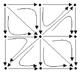
Figure 1: A commutative flow (denoted by curved arrows) on a triangulated digraph. Commutativity of the whole diagram follows from commutativity of its triangular components.

Many properties of mathematical constructions may be represented by universal properties of diagrams [2]. Consider the Cartesian product $X\times Y$ of two sets, consisting as usual of all ordered pairs $\langle x,y\rangle$ of elements $x\in X$ and $y\in Y$. The projections $\langle x,y\rangle\mapsto x,\,\,\langle x,y\rangle\mapsto y$ of the product on its ‘axes’ $X$ and $Y$ are functions $p:X\times Y\rightarrow X,\,\,q:X\times Y\rightarrow Y$. Any function $h:W\rightarrow X\times Y$ from a third set $W$ is uniquely determined by its composites $p\circ h$ and $q\circ h$. Conversely, given $W$ and two functions $f$ and $g$ as in the diagram below, there is a unique function $h$ which makes the following diagram commute:

This property describes the Cartesian product $X\times Y$ uniquely; the same diagram, read in the category of topological spaces or of groups, describes uniquely the Cartesian product of spaces or of the direct product of groups.

The construction ‘Cartesian product’ is technically called a ‘functor’ because it applies suitably both to the sets and to the functions between them; two functions $k:X\rightarrow X^{\prime}$ and $l:Y\rightarrow Y^{\prime}$ have a function $k\times l$ as their Cartesian product:

$$k\times l:X\times Y\rightarrow X^{\prime}\times Y^{\prime},\qquad\langle x,y\rangle\mapsto\langle kx,ly\rangle.$$

3 Categories

A category is a generic mathematical structure consisting of a collection of objects (sets with possibly additional structure), with a corresponding collection of arrows, or morphisms, between objects (agreeing with this additional structure). A category $\mathcal{K}$ is defined as a pair $\left(\mathtt{Ob}(\mathcal{K}),\mathtt{Mor}(\mathcal{K})\right)$ of generic objects $A,B,\ldots$ in $\mathtt{Ob}(\mathcal{K})$ and generic arrows $f:A\rightarrow B,\,g:B\rightarrow C,\ldots$ in $\mathtt{Mor}(\mathcal{K})$ between objects, with associative composition:

$$A{\makebox[42.00003pt]{\rule[-1.49994pt]{0.0pt}{18.88889pt}\raisebox{1.50009pt}{\begin{picture}(4.2,0.4)(-0.3,-0.2)\put(1.8,0.2){\makebox(0.0,0.0)[b]{$f$}}\put(0.0,0.0){\vector(1,0){3.6}}\end{picture}}}}B{\makebox[42.00003pt]{\rule[-1.49994pt]{0.0pt}{16.24998pt}\raisebox{1.50009pt}{\begin{picture}(4.2,0.4)(-0.3,-0.2)\put(1.8,0.2){\makebox(0.0,0.0)[b]{$g$}}\put(0.0,0.0){\vector(1,0){3.6}}\end{picture}}}}C=A{\makebox[42.00003pt]{\rule[-1.49994pt]{0.0pt}{18.88889pt}\raisebox{1.50009pt}{\begin{picture}(4.2,0.4)(-0.3,-0.2)\put(1.8,0.2){\makebox(0.0,0.0)[b]{$g{\raisebox{0.56905pt}{\scriptstyle\circ}}f$}}\put(0.0,0.0){\vector(1,0){3.6}}\end{picture}}}}C,$$

and identity (loop) arrow. (Note that in topological literature, $\mathtt{Hom}(\mathcal{K})$ or $\mathtt{hom}(\mathcal{K})$ is used instead of $\mathtt{Mor}(\mathcal{K})$; see [3]).

A category $\mathcal{K}$ is usually depicted as a commutative diagram (i.e., a diagram with a common initial object $A$ and final object $D$):

To make this more precise, we say that a category $\mathcal{K}$ is defined if we have:

1. A class of objects $\{A,B,C,...\}$ of $\mathcal{K}$, denoted by $\mathtt{Ob}(\mathcal{K});$

2. A set of morphisms, or arrows $\mathtt{Mor}_{\mathcal{K}}(A,B),$ with elements $f:A\rightarrow B$, defined for any ordered pair $(A,B)\in\mathcal{K}$, such that for two different pairs $(A,B)\neq(C,D)$ in $\mathcal{K}$, we have $\mathtt{Mor}_{\mathcal{K}}(A,B)\cap\mathtt{Mor}_{\mathcal{K}}(C,D)=\emptyset$;

3. For any triplet $(A,B,C)\in\mathcal{K}$ with $f:A\rightarrow B$ and $g:B\rightarrow C$, there is a composition of morphisms

   $$\mathtt{Mor}_{\mathcal{K}}(B,C)\times\mathtt{Mor}_{\mathcal{K}}(A,B)\ni(g,f)\rightarrow g\circ f\in\mathtt{Mor}_{\mathcal{K}}(A,C),$$

   written schematically as

   $$\frac{f:A\rightarrow B,\qquad g:B\rightarrow C}{g\circ f:A\rightarrow C}.$$

Recall from above that if we have a morphism $f\in\mathtt{Mor}_{\mathcal{K}}(A,B)$, (otherwise written $f:A\rightarrow B$, or $A{\makebox[42.00003pt]{\rule[-1.49994pt]{0.0pt}{18.88889pt}\raisebox{1.50009pt}{\begin{picture}(4.2,0.4)(-0.3,-0.2)\put(1.8,0.2){\makebox(0.0,0.0)[b]{$f$}}\put(0.0,0.0){\vector(1,0){3.6}}\end{picture}}}}B$), then $A=\mathop{\mathrm{d}om}(f)$ is a domain of $f$, and $B=\mathop{\mathrm{c}od}(f)$ is a codomain of $f$ (of which range of $f$ is a subset, $B=\mathop{\mathrm{r}an}(f)$).

To make $\mathcal{K}$ a category, it must also fulfill the following two properties:

1. Associativity of morphisms: for all $f\in\mathtt{Mor}_{\mathcal{K}}(A,B)$, $g\in\mathtt{Mor}_{\mathcal{K}}(B,C)$, and $h\in\mathtt{Mor}_{\mathcal{K}}(C,D)$, we have $h\circ(g\circ f)=(h\circ g)\circ f$; in other words, the following diagram is commutative

2. Existence of identity morphism: for every object $A\in\mathtt{Ob}(\mathcal{K})$ exists a unique identity morphism $1_{A}\in\mathtt{Mor}_{\mathcal{K}}(A,A)$; for any two morphisms $f\in\mathtt{Mor}_{\mathcal{K}}(A,B)$, and
   $g\in\mathtt{Mor}_{\mathcal{K}}(B,C)$, compositions with identity morphism $1_{B}\in\mathtt{Mor}_{\mathcal{K}}(B,B)$ give $1_{B}\circ f=f$ and $g\circ 1_{B}=g$, i.e., the following diagram is commutative:

The set of all morphisms of the category $\mathcal{K}$ is denoted

$$\mathtt{Mor}(\mathcal{K})=\bigcup_{{A,B\in Ob(\mathcal{K})}}\mathtt{Mor}_{\mathcal{K}}(A,B).$$

If for two morphisms $f\in\mathtt{Mor}_{\mathcal{K}}(A,B)$ and $g\in\mathtt{Mor}_{\mathcal{K}}(B,A)$ the equality $g\circ f=1_{A}$ is valid, then the morphism $g$ is said to be left inverse (or retraction), of $f$, and $f$ right inverse (or section) of $g$. A morphism which is both right and left inverse of $f$ is said to be two–sided inverse of $f$.

A morphism $m:A\rightarrow B$ is called monomorphism in $\mathcal{K}$ (i.e., 1–1, or injection map), if for any two parallel morphisms $f_{1},f_{2}:C\rightarrow A$ in $\mathcal{K}$ the equality $m\circ f_{1}=m\circ f_{2}$ implies $f_{1}=f_{2}$; in other words, $m$ is monomorphism if it is left cancellable. Any morphism with a left inverse is monomorphism.

A morphism $e:A\rightarrow B$ is called epimorphism in $\mathcal{K}$ (i.e., onto, or surjection map), if for any two morphisms $g_{1},g_{2}:B\rightarrow C$ in $\mathcal{K}$ the equality $g_{1}\circ e=g_{2}\circ e$ implies $g_{1}=g_{2}$; in other words, $e$ is epimorphism if it is right cancellable. Any morphism with a right inverse is epimorphism.

A morphism $f:A\rightarrow B$ is called isomorphism in $\mathcal{K}$ (denoted as $f:A\cong B$) if there exists a morphism $f^{-1}:B\rightarrow A$ which is a two–sided inverse of $f$ in $\mathcal{K}$. The relation of isomorphism is reflexive, symmetric, and transitive, that is, an equivalence relation.

For example, an isomorphism in the category of sets is called a set–isomorphism, or a bijection, in the category of topological spaces is called a topological isomorphism, or a homeomorphism, in the category of differentiable manifolds is called a differentiable isomorphism, or a diffeomorphism.

A morphism $f\in\mathtt{Mor}_{\mathcal{K}}(A,B)$ is regular if there exists a morphism $g:B\rightarrow A$ in $\mathcal{K}$ such that $f\circ g\circ f=f$. Any morphism with either a left or a right inverse is regular.

An object $T$ is a terminal object in $\mathcal{K}$ if to each object $A\in\mathtt{Ob}(\mathcal{K})$ there is exactly one arrow $A\rightarrow T$. An object $S$ is an initial object in $\mathcal{K}$ if to each object $A\in\mathtt{Ob}(\mathcal{K})$ there is exactly one arrow $S\rightarrow A$. A null object $Z\in\mathtt{Ob}(\mathcal{K})$ is an object which is both initial and terminal; it is unique up to isomorphism. For any two objects $A,B\in\mathtt{Ob}(\mathcal{K})$ there is a unique morphism $A\rightarrow Z\rightarrow B$ (the composite through $Z$), called the zero morphism from $A$ to $B$.

A notion of subcategory is analogous to the notion of subset. A subcategory $\mathcal{L}$ of a category $\mathcal{K}$ is said to be a complete subcategory iff for any objects $A,B\in\mathcal{L}$, every morphism $A\rightarrow B$ of $\mathcal{L}$ is in $\mathcal{K}$.

A groupoid is a category in which every morphism is invertible. A typical groupoid is the fundamental groupoid $\Pi_{1}(X)$ of a topological space $X$. An object of $\Pi_{1}(X)$ is a point $x\in X$, and a morphism $x\rightarrow x^{\prime}$ of $\Pi_{1}(X)$ is a homotopy class of paths $f$ from $x$ to $x^{\prime}$. The composition of paths $g:x^{\prime}\rightarrow x^{\prime\prime}$ and $f:x\rightarrow x^{\prime}$ is the path $h$ which is ‘$f$ followed by $g$’. Composition applies also to homotopy classes, and makes $\Pi_{1}(X)$ a category and a groupoid (the inverse of any path is the same path traced in the opposite direction).

A group is a groupoid with one object, i.e., a category with one object in which all morphisms are isomorphisms (see Appendix). Therefore, if we try to generalize the concept of a group, keeping associativity as an essential property, we get the notion of a category.

A category is discrete if every morphism is an identity. A monoid is a category with one object, which is a group without inverses. A group is a category with one object in which every morphism has a two–sided inverse under composition.

Homological algebra was the progenitor of category theory (see e.g., [8]). Generalizing L. Euler’s formula: $f+v=e+2$, for the faces $f$, vertices $v$ and edges $e$ of a convex polyhedron, E. Betti defined numerical invariants of spaces by formal addition and subtraction of faces of various dimensions. H. Poincaré formalized these and introduced the concept of homology. E. Noether stressed the fact that these calculations go on in Abelian groups, and that the operation $\partial_{n}$ taking a face of dimension $n$ to the alternating sum of faces of dimension $n-1$ which form its boundary is a homomorphism, and it also satisfies the boundary of a boundary is zero rule: $\partial_{n}\circ\partial_{n+1}=0$. There are many ways of approximating a given space by polyhedra, but the quotient $H_{n}=\mathop{\mathrm{K}er}\partial_{n}/\mathop{\mathrm{I}m}\partial_{n+1}$ is an invariant, the homology group.

As a physical example from [12, 13], consider some physical system of type $A$ (e.g., an electron) and perform some physical operation $f$ on it (e.g., perform a measurement on it), which results in a possibly different system $B$ (e.g., a perturbed electron), thus having a map $f:A\allowbreak\mathrel{\mathop{\hbox to11.99998pt{\rightarrowfill}}\limits}B$. In a same way, we can perform a consecutive operation $g:B\allowbreak\mathrel{\mathop{\hbox to11.99998pt{\rightarrowfill}}\limits}C$ (e.g., perform the second measurement, this time on $B$), possibly resulting in a different system $C$ (e.g., a secondly perturbed electron). Thus, we have a composition: $k=g\circ f$, representing the consecutive application of these two physical operations, or the following diagram commutes:

In a similar way, we can perform another consecutive operation $h:C\allowbreak\mathrel{\mathop{\hbox to11.99998pt{\rightarrowfill}}\limits}D$ (e.g., perform the third measurement, this time on $C$), possibly resulting in a different system $D$ (e.g., a thirdly perturbed electron). Clearly we have an associative composition $(h\circ g)\circ f=h\circ(g\circ f)$, or the following diagram commutes:

Finally, if we introduce a trivial operation $1_{A}\in\mathtt{Mor}_{\mathcal{K}}(A,A)$, meaning ‘doing nothing on a system of type $A$’, we have $1_{B}\circ f=f\circ 1_{A}=f$. In this way, we have constructed a generic physical category (for more details, see [12, 13]).

For the same operational reasons, categories could be expected to play an important role in other fields where operations/processes play a central role: e.g., Computer Science (computer programs as morphisms) and Logic & Proof Theory (proofs as morphisms). In the theoretical counterparts to these fields category theory has become quite common practice (see [14]).

4 Functors

In algebraic topology, one attempts to assign to every topological space $X$ some algebraic object $\mathcal{F}(X)$ in such a way that to every $C^{0}-$function $f:X\rightarrow Y$ there is assigned a homomorphism $\mathcal{F}(f):\mathcal{F}(X)\allowbreak\mathrel{\mathop{\hbox to11.99998pt{\rightarrowfill}}\limits}\mathcal{F}(Y)$ (see [3, 4]). One advantage of this procedure is, e.g., that if one is trying to prove the non–existence of a $C^{0}-$function $f:X\rightarrow Y$ with certain properties, one may find it relatively easy to prove the non–existence of the corresponding algebraic function $\mathcal{F}(f)$ and hence deduce that $f$ could not exist. In other words, $\mathcal{F}$ is to be a ‘homomorphism’ from one category (e.g., $\mathcal{T}$) to another (e.g., $\mathcal{G}$ or $\mathcal{A}$). Formalization of this notion is a functor.

A functor is a generic picture projecting (all objects and morphisms of) a source category into a target category. Let $\mathcal{K}=\left(\mathtt{Ob}(\mathcal{K}),\mathtt{Mor}(\mathcal{K})\right)$ be a source (or domain) category and $\mathcal{L}=\left(\mathtt{Ob}(\mathcal{L}),\mathtt{Mor}(\mathcal{L})\right)$ be a target (or codomain) category. A functor $\mathcal{F}=(\mathcal{F}_{O},\mathcal{F}_{M})$ is defined as a pair of maps, $\mathcal{F}_{O}:\mathtt{Ob}(\mathcal{K})\rightarrow\mathtt{Ob}(\mathcal{L})$ and $\mathcal{F}_{M}:\mathtt{Mor}(\mathcal{K})\rightarrow\mathtt{Mor}(\mathcal{L})$, preserving categorical symmetry (i.e., commutativity of all diagrams) of $\mathcal{K}$ in $\mathcal{L}$.

More precisely, a covariant functor, or simply a functor, $\mathcal{F}_{\ast}:\mathcal{K}\rightarrow\mathcal{L}$ is a picture in the target category $\mathcal{L}$ of (all objects and morphisms of) the source category $\mathcal{K}$:

Similarly, a contravariant functor, or a cofunctor, $\mathcal{F}^{\ast}:\mathcal{K}\rightarrow\mathcal{L}$ is a dual picture with reversed arrows:

In other words, a functor $\mathcal{F}:\mathcal{K}\rightarrow\mathcal{L}$ from a source category $\mathcal{K}$ to a target category $\mathcal{L}$, is a pair $\mathcal{F}=(\mathcal{F}_{O},\mathcal{F}_{M})$ of maps $\mathcal{F}_{O}:\mathtt{Ob}(\mathcal{K})\rightarrow\mathtt{Ob}(\mathcal{L})$, $\mathcal{F}_{M}:\mathtt{Mor}(\mathcal{K})\rightarrow\mathtt{Mor}(\mathcal{L})$, such that

1. If $f\in\mathtt{Mor}_{\mathcal{K}}(A,B)$ then $\mathcal{F}_{M}(f)\in\mathtt{Mor}_{\mathcal{L}}(\mathcal{F}_{O}(A),\mathcal{F}_{O}(B))$ in case of the covariant functor $\mathcal{F}_{\ast}$, and $\mathcal{F}_{M}(f)\in\mathtt{Mor}_{\mathcal{L}}(\mathcal{F}_{O}(B),\mathcal{F}_{O}(A))$ in case of the contravariant functor $\mathcal{F}^{\ast}$;

2. For all $A\in\mathtt{Ob}(\mathcal{K}):$ $\mathcal{F}_{M}(1_{A})=1_{\mathcal{F}_{O}(A)};$

3. For all $f,g\in\mathtt{Mor}(\mathcal{K})$: if $\mathop{\mathrm{c}od}(f)=\mathop{\mathrm{d}om}(g)$, then $\mathcal{F}_{M}(g\circ f)=\mathcal{F}_{M}(g)\circ\mathcal{F}_{M}(f)$ in case of the covariant functor $\mathcal{F}_{\ast}$, and $\mathcal{F}_{M}(g\circ f)=\mathcal{F}_{M}(f)\circ\mathcal{F}_{M}(g)$ in case of the contravariant functor $\mathcal{F}^{\ast}$.

Category theory originated in algebraic topology, which tried to assign algebraic invariants to topological structures. The golden rule of such invariants is that they should be functors. For example, the fundamental group $\pi_{1}$ is a functor. Algebraic topology constructs a group called the fundamental group $\pi_{1}(X)$ from any topological space $X$, which keeps track of how many holes the space $X$ has. But also, any map between topological spaces determines a homomorphism $\phi:\pi_{1}(X)\rightarrow\pi_{1}(Y)$ of the fundamental groups. So the fundamental group is really a functor $\pi_{1}:\mathcal{T}\rightarrow\mathcal{G}$. This allows us to completely transpose any situation involving spaces and continuous maps between them to a parallel situation involving groups and homomorphisms between them, and thus reduce some topology problems to algebra problems.

Also, singular homology in a given dimension $n$ assigns to each topological space $X$ an Abelian group $H_{n}(X)$, its $n$th homology group of $X$, and also to each continuous map $f:X\rightarrow Y$ of spaces a corresponding homomorphism $H_{n}(f):H_{n}(X)\rightarrow H_{n}(Y)$ of groups, and this in such a way that $H_{n}(X)$ becomes a functor $H_{n}:\mathcal{T}\rightarrow\mathcal{A}$.

The leading idea in the use of functors in topology is that $H_{n}$ or $\pi_{n}$ gives an algebraic picture or image not just of the topological spaces $X,Y$ but also of all the continuous maps $f:X\rightarrow Y$ between them.

Similarly, there is a functor $\Pi_{1}:\mathcal{T}\rightarrow\mathcal{G}$, called the ‘fundamental groupoid functor’, which plays a very basic role in algebraic topology. Here’s how we get from any space $X$ its ‘fundamental groupoid’ $\Pi_{1}(X)$. To say what the groupoid $\Pi_{1}(X)$ is, we need to say what its objects and morphisms are. The objects in $\Pi_{1}(X)$ are just the points of $X$ and the morphisms are just certain equivalence classes of paths in $X$. More precisely, a morphism $f:x\rightarrow y$ in $\Pi_{1}(X)$ is just an equivalence class of continuous paths from $x$ to $y$, where two paths from $x$ to $y$ are decreed equivalent if one can be continuously deformed to the other while not moving the endpoints. (If this equivalence relation holds, we say the two paths are ‘homotopic’, and we call the equivalence classes ‘homotopy classes of paths’; see [2, 3]).

Another examples are covariant forgetful functors:

• From the category of topological spaces to the category of sets; it ‘forgets’ the topology–structure.

• From the category of metric spaces to the category of topological spaces with the topology induced by the metrics; it ‘forgets’ the metric.

For each category $\mathcal{K}$, the identity functor $I_{\mathcal{K}}$ takes every $\mathcal{K}-$object and every $\mathcal{K}-$morphism to itself.

Given a category $\mathcal{K}$ and its subcategory $\mathcal{L}$, we have an inclusion functor $\mathtt{In}:\mathcal{L}\allowbreak\mathrel{\mathop{\hbox to11.99998pt{\rightarrowfill}}\limits}\mathcal{K}$.

Given a category $\mathcal{K}$, a diagonal functor $\Delta:\mathcal{K}\allowbreak\mathrel{\mathop{\hbox to11.99998pt{\rightarrowfill}}\limits}\mathcal{K}\times\mathcal{K}$ takes each object $A\in\mathcal{K}$ to the object $(A,A)$ in the product category $\mathcal{K}\times\mathcal{K}$.

Given a category $\mathcal{K}$ and a category of sets $\mathcal{S}$, each object $A\in\mathcal{K}$ determines a covariant Hom–functor $\mathcal{K}[A,\_]:\mathcal{K}\rightarrow\mathcal{S}$, a contravariant Hom–functor $\mathcal{K}[\_,A]:\mathcal{K}\allowbreak\mathrel{\mathop{\hbox to11.99998pt{\rightarrowfill}}\limits}\mathcal{S}$, and a Hom–bifunctor $\mathcal{K}[\_,\_]:\mathcal{K}^{op}\times\mathcal{K}\rightarrow\mathcal{S}$.

A functor $\mathcal{F}:\mathcal{K}\rightarrow\mathcal{L}$ is a faithful functor if for all $A,B\in\mathtt{Ob}(\mathcal{K})$ and for all $f,g\in\mathtt{Mor}_{\mathcal{K}}(A,B)$, $\mathcal{F}(f)=\mathcal{F}(g)$ implies $f=g$; it is a full functor if for every $h\in\mathtt{Mor}_{\mathcal{L}}(\mathcal{F}(A),\mathcal{F}(B))$, there is $g\in\mathtt{Mor}_{\mathcal{K}}(A,B)$ such that $h=\mathcal{F}(g)$; it is a full embedding if it is both full and faithful.

A representation of a group is a functor $\mathcal{F}:\mathcal{G}\rightarrow\mathcal{V}$. Thus, a category is a generalization of a group and group representations are a special case of category representations.

5 Natural Transformations

A natural transformation (i.e., a functor morphism) $\mathbf{\tau}:\mathcal{F}\overset{\cdot}{\rightarrow}\mathcal{G}$ is a map between two functors of the same variance, $(\mathcal{F},\mathcal{G}):\mathcal{K}\rightrightarrows\mathcal{L}$, preserving categorical symmetry:

More precisely, all functors of the same variance from a source category $\mathcal{K}$ to a target category $\mathcal{L}$ form themselves objects of the functor category $\mathcal{L}^{\mathcal{K}}$. Morphisms of $\mathcal{L}^{\mathcal{K}}$, called natural transformations, are defined as follows.

Let $\mathcal{F}:\mathcal{K}\rightarrow\mathcal{L}$ and $\mathcal{G}:\mathcal{K}\rightarrow\mathcal{L}$ be two functors of the same variance from a category $\mathcal{K}$ to a category $\mathcal{L}$. Natural transformation $\mathcal{F\overset{\mathbf{\tau}}{\longrightarrow}G}$ is a family of morphisms such that for all $f\in\mathtt{Mor}_{\mathcal{K}}(A,B)$ in the source category $\mathcal{K}$, we have $\mathcal{G}(f)\circ\mathbf{\tau}_{A}=\mathbf{\tau}_{B}\circ\mathcal{F}(f)$ in the target category $\mathcal{L}$. Then we say that the component $\mathbf{\tau}_{A}:\mathcal{F}(A)\rightarrow\mathcal{G}(A)$ is natural in $A$.

If we think of a functor $\mathcal{F}$ as giving a picture in the target category $\mathcal{L}$ of (all the objects and morphisms of) the source category $\mathcal{K}$, then a natural transformation $\mathbf{\tau}$ represents a set of morphisms mapping the picture $\mathcal{F}$ to another picture $\mathcal{G}$, preserving the commutativity of all diagrams.

An invertible natural transformation, such that all components $\mathbf{\tau}_{A}$ are isomorphisms) is called a natural equivalence (or, natural isomorphism). In this case, the inverses $(\mathbf{\tau}_{A})^{-1}$ in $\mathcal{L}$ are the components of a natural isomorphism $(\mathbf{\tau})^{-1}:\mathcal{G}\overset{\ast}{\longrightarrow}\mathcal{F}$. Natural equivalences are among the most important metamathematical constructions in algebraic topology (see [3]).

As a mathematical example, let $\mathcal{B}$ be the category of Banach spaces over $\mathbb{R}$ and bounded linear maps. Define $D:\mathcal{B}\rightarrow\mathcal{B}$ by taking $D(X)=X^{\ast}=$ Banach space of bounded linear functionals on a space $X$ and $D(f)=f^{\ast}$ for $f:X\rightarrow Y$ a bounded linear map. Then $D$ is a cofunctor. $D^{2}=D\circ D$ is also a functor. We also have the identity functor $1:\mathcal{B}\rightarrow\mathcal{B}$. Define $T:1\rightarrow D\circ D$ as follows: for every $X\in\mathcal{B}$ let $T(X):X\rightarrow D^{2}X=X^{\ast\ast}$ be the natural inclusion – that is, for $x\in X$ we have $[T(X)(x)](f)=f(x)$ for every $f\in X^{\ast}$. $T$ is a natural transformation. On the subcategory of $n$D Banach spaces $T$ is even a natural equivalence. The largest subcategory of $\mathcal{B}$ on which $T$ is a natural equivalence is called the category of reflexive Banach spaces [3].

As a physical example, when we want to be able to conceive two physical systems $A$ and $B$ as one whole (see [12, 13]), we can denote this using a (symmetric) monoidal tensor product $A\otimes B$, and hence also need to consider the compound operations

$$A\otimes B{\makebox[42.00003pt]{\rule[-1.49994pt]{0.0pt}{18.88889pt}\raisebox{1.50009pt}{\begin{picture}(4.2,0.4)(-0.3,-0.2)\put(1.8,0.2){\makebox(0.0,0.0)[b]{$f\otimes g$}}\put(0.0,0.0){\vector(1,0){3.6}}\end{picture}}}}C\otimes D,$$

inherited from the operations on the individual systems. Now, a (symmetric) monoidal category is a category $\mathcal{K}$ defined as a pair $\left(\mathtt{Ob}(\mathcal{K}),\mathtt{Mor}(\mathcal{K})\right)$ of generic objects $A,B,\ldots$ in $\mathtt{Ob}(\mathcal{K})$ and generic arrows $f:A\rightarrow B,\,g:B\rightarrow C,\ldots$ in $\mathtt{Mor}(\mathcal{K})$ between objects, defined using the symmetric monoidal tensor product:

$$\mathtt{Ob}(\mathcal{K}) : \{A,B\}~{}\mapsto~{}A\otimes B,$$

$$\mathtt{Mor}(\mathcal{K}) : \{A{\makebox[42.00003pt]{\rule[-1.49994pt]{0.0pt}{18.88889pt}\raisebox{1.50009pt}{\begin{picture}(4.2,0.4)(-0.3,-0.2)\put(1.8,0.2){\makebox(0.0,0.0)[b]{$f$}}\put(0.0,0.0){\vector(1,0){3.6}}\end{picture}}}}B,C{\makebox[42.00003pt]{\rule[-1.49994pt]{0.0pt}{16.24998pt}\raisebox{1.50009pt}{\begin{picture}(4.2,0.4)(-0.3,-0.2)\put(1.8,0.2){\makebox(0.0,0.0)[b]{$g$}}\put(0.0,0.0){\vector(1,0){3.6}}\end{picture}}}}D\}~{}\mapsto~{}A\otimes C{\makebox[42.00003pt]{\rule[-1.49994pt]{0.0pt}{18.88889pt}\raisebox{1.50009pt}{\begin{picture}(4.2,0.4)(-0.3,-0.2)\put(1.8,0.2){\makebox(0.0,0.0)[b]{$f\otimes g$}}\put(0.0,0.0){\vector(1,0){3.6}}\end{picture}}}}B\otimes D,$$

with the additional notion of bifunctoriality: if we apply an operation $f$ to one system and an operation $g$ to another system, then the order in which we apply them does not matter; that is, the following diagram commutes:

which shows that both paths yield the same result (see [12, 13] for technical details).

As ‘categorical fathers’, S. Eilenberg and S. MacLane, first observed, ‘category’ has been defined in order to define ‘functor’ and ‘functor’ has been defined in order to define ‘natural transformations’ [1, 2]).

5.1 Compositions of Natural Transformations

Natural transformations can be composed in two different ways. First, we have an ‘ordinary’ composition: if $\mathcal{F},\mathcal{G}$ and $\mathcal{H}$ are three functors from the source category $\mathcal{A}\$to the target category $\mathcal{B}$, and then $\mathbf{\alpha}:\mathcal{F}\overset{\cdot}{\rightarrow}\mathcal{G}$, $\mathbf{\beta}:\mathcal{G}\overset{\cdot}{\rightarrow}\mathcal{H}$ are two natural transformations, then the formula

$$\left(\beta\circ\alpha\right)_{A}=\beta_{A}\circ\alpha_{A},\text{ \ \ \ \ \ \ (for all }A\in\mathcal{A}),$$ (2)

defines a new natural transformation $\beta\circ\alpha:\mathcal{F}\overset{\cdot}{\rightarrow}\mathcal{H}$. This composition law is clearly associative and possesses a unit $1_{\mathcal{F}}$ at each functor $\mathcal{F}$, whose $\mathcal{A}$–component is $1_{\mathcal{FA}}.$

Second, we have the Godement product of natural transformations, usually denoted by $\ast$. Let $\mathcal{A}$, $\mathcal{B}$ and $\mathcal{C}$ be three categories, $\mathcal{F},\mathcal{G}$, $\mathcal{H}$ and $\mathcal{K}$ be four functors such that $(\mathcal{F},\mathcal{G}):\mathcal{A}\rightrightarrows\mathcal{B}$ and $(\mathcal{H},\mathcal{K}):\mathcal{B}\rightrightarrows\mathcal{C}$, and $\mathbf{\alpha}:\mathcal{F}\overset{\cdot}{\rightarrow}\mathcal{G}$, $\mathbf{\beta}:\mathcal{H}\overset{\cdot}{\rightarrow}\mathcal{K}$ be two natural transformations. Now, instead of (2), the Godement composition is given by

$$\left(\beta\ast\alpha\right)_{A}=\beta_{GA}\circ H\left(\alpha_{A}\right)=K\left(\alpha_{A}\right)\circ\beta_{FA},\text{ \ \ \ \ \ \ (for all }A\in\mathcal{A}),$$ (3)

which defines a new natural transformation $\beta\ast\alpha:\mathcal{H}\circ\mathcal{F}\overset{\cdot}{\rightarrow}\mathcal{K}\circ\mathcal{G}$.

Finally, the two compositions (2) and (3) of natural transformations can be combined as

$$\left(\delta\ast\gamma\right)\circ\left(\beta\ast\alpha\right)=\left(\delta\circ\beta\right)\ast\left(\gamma\circ\alpha\right),$$

where $\mathcal{A}$, $\mathcal{B}$ and $\mathcal{C}$ are three categories, $\mathcal{F},\mathcal{G}$, $\mathcal{H}$, $\mathcal{K}$, $\mathcal{L}$, $\mathcal{M}$ are six functors, and $\mathbf{\alpha}:\mathcal{F}\overset{\cdot}{\rightarrow}\mathcal{H}$, $\mathbf{\beta}:\mathcal{G}\overset{\cdot}{\rightarrow}\mathcal{K}$, $\mathbf{\gamma}:\mathcal{H}\overset{\cdot}{\rightarrow}\mathcal{L}$, $\mathbf{\delta}:\mathcal{K}\overset{\cdot}{\rightarrow}\mathcal{M}$ are four natural transformations.

5.2 Dinatural Transformations

Double natural transformations are called dinatural transformations. An end of a functor $S:C^{op}\times C\rightarrow X$ is a universal dinatural transformation from a constant $e$ to $S$. In other words, an end of $S$ is a pair $\langle e,\omega\rangle$, where $e$ is an object of $X$ and $\omega:e\overset{..}{\rightarrow}S$ is a wedge (dinatural) transformation with the property that to every wedge $\beta:x\overset{..}{\rightarrow}S$ there is a unique arrow $h:x\rightarrow e$ of $B$ with $\beta_{c}=\omega_{c}h$ for all $a\in C$. We call $\omega$ the ending wedge with components $\omega_{c}$, while the object $e$ itself, by abuse of language, is called the end of $S$ and written with integral notation as $\int\limits_{c}S(c,c)$; thus

$$S(c,c)\overset{\omega_{c}}{\rightarrow}\int\limits_{c}S(c,c)=e.$$

Note that the ‘variable of integration’ $c$ appears twice under the integral sign (once contravariant, once covariant) and is ‘bound’ by the integral sign, in that the result no longer depends on $c$ and so is unchanged if ‘$c$’ is replaced by any other letter standing for an object of the category $C$. These properties are like those of the letter $x$ under the usual integral symbol $\int f(x)\,dx$ of calculus.

Every end is manifestly a limit (see below) – specifically, a limit of a suitable diagram in $X$ made up of pieces like $S(b,b)\rightarrow S(b,c)\rightarrow S(c,c)$.

For each functor $T:C\rightarrow X$ there is an isomorphism

$$\int\limits_{c}S(c,c)=\int\limits_{c}Tc\cong\mathop{\mathrm{L}im}T,$$

valid when either the end of the limit exists, carrying the ending wedge to the limiting cone; the indicated notation thus allows us to write any limit as an integral (an end) without explicitly mentioning the dummy variable (the first variable $c$ of $S$).

A functor $H:X\rightarrow Y$ is said to preserve the end of a functor $S:C^{op}\times C\rightarrow X$ when $\omega:e\overset{..}{\rightarrow}S$ an end of $S$ in $X$ implies that $H\omega:He\overset{..}{\rightarrow}HS$ is an and for $HS$; in symbols

$$H\int\limits_{c}S(c,c)=\int\limits_{c}HS(c,c).$$

Similarly, $H$ creates the end of $S$ when to each end $v:y\overset{..}{\rightarrow}HS$ in $Y$ there is a unique wedge $\omega:e\overset{..}{\rightarrow}S$ with $H\omega=v$, and this wedge $\omega$ is an end of $S.$

The definition of the coend of a functor $S:C^{op}\times C\rightarrow X$ is dual to that of an end. A coend of $S$ is a pair $\langle d,\zeta\rangle$, consisting of an object $d\in X$ and a wedge $\zeta:S\overset{..}{\rightarrow}d$. The object $d$ (when it exists, unique up to isomorphism) will usually be written with an integral sign and with the bound variable $c$ as superscript; thus

$$S(c,c)\overset{\zeta_{c}}{\rightarrow}\int\limits^{c}S(c,c)=d.$$

The formal properties of coends are dual to those of ends. Both are much like those for integrals in calculus (see [2], for technical details).

6 Limits and Colimits

In abstract algebra constructions are often defined by an abstract property which requires the existence of unique morphisms under certain conditions. These properties are called universal properties. The limit of a functor generalizes the notions of inverse limit and product used in various parts of mathematics. The dual notion, colimit, generalizes direct limits and direct sums. Limits and colimits are defined via universal properties and provide many examples of adjoint functors.

A limit of a covariant functor $\mathcal{F}:\mathcal{J}\rightarrow\mathcal{C}$ is an object $L$ of $\mathcal{C}$, together with morphisms $\phi_{X}:L\rightarrow\mathcal{F}(X)$ for every object $X$ of $\mathcal{J}$, such that for every morphism $f:X\rightarrow Y$ in $\mathcal{J}$, we have $\mathcal{F}(f)\phi_{X}=\phi_{Y}$, and such that the following universal property is satisfied: for any object $N$ of $\mathcal{C}$ and any set of morphisms $\psi_{X}:N\rightarrow\mathcal{F}(X)$ such that for every morphism $f:X\rightarrow Y$ in $\mathcal{J}$, we have $\mathcal{F}(f)\psi_{X}=\psi_{Y}$, there exists precisely one morphism $u:N\rightarrow L$ such that $\phi_{X}u=\psi_{X}$ for all $X$. If $\mathcal{F}$ has a limit (which it need not), then the limit is defined up to a unique isomorphism, and is denoted by $\lim\mathcal{F}$.

Analogously, a colimit of the functor $\mathcal{F}:\mathcal{J}\rightarrow\mathcal{C}$ is an object $L$ of $\mathcal{C}$, together with morphisms $\phi_{X}:\mathcal{F}(X)\rightarrow L$ for every object $X$ of $\mathcal{J}$, such that for every morphism $f:X\rightarrow Y$ in $\mathcal{J}$, we have $\phi_{Y}\mathcal{F}(X)=\phi_{X}$, and such that the following universal property is satisfied: for any object $N$ of $\mathcal{C}$ and any set of morphisms $\psi_{X}:\mathcal{F}(X)\rightarrow N$ such that for every morphism $f:X\rightarrow Y$ in $\mathcal{J}$, we have $\psi_{Y}\mathcal{F}(X)=\psi_{X}$, there exists precisely one morphism $u:L\rightarrow N$ such that $u\phi_{X}=\psi_{X}$ for all $X$. The colimit of $\mathcal{F}$, unique up to unique isomorphism if it exists, is denoted by $\mathop{\mathrm{c}olim}\mathcal{F}$.

Limits and colimits are related as follows: A functor $\mathcal{F}:\mathcal{J}\rightarrow\mathcal{C}$ has a colimit iff for every object $N$ of $\mathcal{C}$, the functor $X\longmapsto Mor_{\mathcal{C}}(\mathcal{F}(X),N)$ (which is a covariant functor on the dual category $\mathcal{J}^{op}$) has a limit. If that is the case, then $Mor_{\mathcal{C}}(\mathop{\mathrm{c}olim}\mathcal{F},N)=\lim Mor_{\mathcal{C}}(\mathcal{F}(-),N)$ for every object $N$ of $\mathcal{C}$.

7 Adjunction

The most important functorial operation is adjunction; as S. MacLane once said, “Adjoint functors arise everywhere” [2].

The adjunction $\mathbf{\varphi}:\mathcal{F}\dashv\mathcal{G}$ between two functors $(\mathcal{F},\mathcal{G}):\mathcal{K}\leftrightarrows\mathcal{L}$ of opposite variance [9], represents a weak functorial inverse:

$$\frac{f:\mathcal{F}(A)\rightarrow B}{\mathbf{\varphi}(f):A\rightarrow\mathcal{G}(B)},$$

forming a natural equivalence $\mathbf{\varphi}:\mathtt{Mor}_{\mathcal{K}}(\mathcal{F}(A),B)\overset{\mathbf{\varphi}}{\longrightarrow}\mathtt{Mor}_{\mathcal{L}}(A,\mathcal{G}(B)).$ The adjunction isomorphism is given by a bijective correspondence (a 1–1 and onto map on objects) $\mathbf{\varphi}:\mathtt{Mor}(\mathcal{K})\ni f\rightarrow\mathbf{\varphi}(f)\in\mathtt{Mor}(\mathcal{L})$ of isomorphisms in the two categories, $\mathcal{K}$ (with a representative object $A$), and $\mathcal{L}$ (with a representative object $B$). It can be depicted as a non–commutative diagram

In this case $\mathcal{F}$ is called left adjoint, while $\mathcal{G}$ is called right adjoint.

In other words, an adjunction $F\dashv G$ between two functors $(\mathcal{F},\mathcal{G})$ of opposite variance, from a source category $\mathcal{K}$ to a target category $\mathcal{L}$, is denoted by $(\mathcal{F},\mathcal{G},\mathbf{\eta},\mathbf{\varepsilon}):\mathcal{K}\leftrightarrows\mathcal{L}$. Here, $\mathcal{F}:\mathcal{L}\rightarrow\mathcal{K}$ is the left (upper) adjoint functor, $\mathcal{G}:\mathcal{K}\leftarrow\mathcal{L}$ is the right (lower) adjoint functor, $\mathbf{\eta}:1_{\mathcal{L}}\rightarrow\mathcal{G}\circ\mathcal{F}$ is the unit natural transformation (or, front adjunction), and $\mathbf{\varepsilon}:\mathcal{F}\circ\mathcal{G}\rightarrow 1_{\mathcal{K}}$ is the counit natural transformation (or, back adjunction).

For example, $\mathcal{K}=\mathcal{S}$ is the category of sets and $\mathcal{L}=\mathcal{G}$ is the category of groups. Then $\mathcal{F}$ turns any set into the free group on that set, while the ‘forgetful’ functor $\mathcal{F}^{\ast}$ turns any group into the underlying set of that group. Similarly, all sorts of other ‘free’ and ‘underlying’ constructions are also left and right adjoints, respectively.

Right adjoints preserve limits, and left adjoints preserve colimits.

The category $\mathcal{C}$ is called a cocomplete category if every functor $\mathcal{F}:\mathcal{J}\rightarrow\mathcal{C}$ has a colimit. The following categories are cocomplete: $\mathcal{S},\mathcal{G},\mathcal{A},\mathcal{T},$ and $\mathcal{PT}.$

The importance of adjoint functors lies in the fact that every functor which has a left adjoint (and therefore is a right adjoint) is continuous. In the category $\mathcal{A}$ of Abelian groups, this shows e.g. that the kernel of a product of homomorphisms is naturally identified with the product of the kernels. Also, limit functors themselves are continuous. A covariant functor $\mathcal{F}:\mathcal{J}\rightarrow\mathcal{C}$ is co-continuous if it transforms colimits into colimits. Every functor which has a right adjoint (and therefore is a left adjoint) is co-continuous.

7.1 Application: Physiological Sensory–Motor Adjunction

Recall that sensations from the skin, muscles, and internal organs of the body, are transmitted to the central nervous system via axons that enter via spinal nerves. They are called sensory pathways. On the other hand, the motor system executes control over the skeletal muscles of the body via several major tracts (including pyramidal and extrapyramidal). They are called motor pathways. Sensory–motor (or, sensorimotor) control/coordination concerns relationships between sensation and movement or, more broadly, between perception and action. The interplay of sensory and motor processes provides the basis of observable human behavior. Anatomically, its top–level, association link can be visualized as a talk between sensory and motor Penfield’s homunculi. This sensory–motor control system can be modelled as an adjunction between the afferent sensory functor $\mathcal{S}:\mathcal{BODY}\allowbreak\mathrel{\mathop{\hbox to11.99998pt{\rightarrowfill}}\limits}\mathcal{BRAIN}$ and the efferent motor functor $\mathcal{M}:\mathcal{BRAIN}\allowbreak\mathrel{\mathop{\hbox to11.99998pt{\rightarrowfill}}\limits}\mathcal{BODY}$. Thus, we have $\mathcal{SMC}:\mathcal{S}\dashv\mathcal{M}$, with $(\mathcal{S},\mathcal{M}):\mathcal{BRAIN}\leftrightarrows\mathcal{BODY}$ and depicted as

This adjunction offers a mathematical answer to the fundamental question: How would Nature solve a general biodynamics control/coordination problem? By using a weak functorial inverse of sensory neural pathways and motor neural pathways, Nature controls human behavior in general, and human motion in particular.

More generally, normal functioning of human body is achieved through interplay of a number of physiological systems – Objects of the category BODY: musculoskeletal system, circulatory system, gastrointestinal system, integumentary system, urinary system, reproductive system, immune system and endocrine system. These systems are all interrelated, so one can say that the Morphisms between them make the proper functioning of the BODY as a whole. On the other hand, BRAIN contains the images of all above functional systems (Brain objects) and their interrelations (Brain morphisms), for the purpose of body control. This body–control performed by the brain is partly unconscious, through neuro–endocrine complex, and partly conscious, through neuro–muscular complex. A generalized sensory functor $\mathcal{SS}$ sends the information about the state of all Body objects (at any time instant) to their images in the Brain. A generalized motor functor $\mathcal{MM}$ responds to these upward sensory signals by sending downward corrective action–commands from the Brain’s objects and morphisms to the Body’s objects and morphisms.

For physiological details, see [10]. For other bio–physical applications of categorical meta-language, see [11, 4, 5].

8 Appendix: Groups and Related Algebraic Structures

As already stated, the basic functional unit of lower biomechanics is the special Euclidean group $SE(3)$ of rigid body motions. In general, a group is a pointed set $(G,e)$ with a multiplication $\mu:G\times G\rightarrow G$ and an inverse $\nu:G\rightarrow G$ such that the following diagrams commute [3]:

1. ($e$ is a two–sided identity)

2. (associativity)

3. (inverse).

Here $e:G\rightarrow G$ is the constant map $e(g)=e$ for all $g\in G$. $(e,1)$ means the map such that $(e,1)(g)=(e,g)$, etc. A group $G$ is called commutative or Abelian group if in addition the following diagram commutes

where $T:G\times G\rightarrow G\times G$ is the switch map $T(g_{1},g_{2})=(g_{2},g_{1}),$ for all $(g_{1},g_{2})\in G\times G.$

A group $G$ acts (on the left) on a set $A$ if there is a function $\alpha:G\times A\rightarrow A$ such that the following diagrams commute [3]:

2. where $(e,1)(x)=(e,x)$ for all $x\in A$. The orbits of the action are the sets $Gx=\{gx:g\in G\}$ for all $x\in A$.

Given two groups $(G,\ast)$ and $(H,\cdot)$, a group homomorphism from $(G,\ast)$ to $(H,\cdot)$ is a function $h:G\rightarrow H$ such that for all $x$ and $y$ in $G$ it holds that

$$h(x\ast y)=h(x)\cdot h(y).$$

From this property, one can deduce that $h$ maps the identity element $e_{G}$ of $G$ to the identity element $e_{H}$ of $H$, and it also maps inverses to inverses in the sense that $h(x^{-1})=h(x)^{-1}$. Hence one can say that $h$ is compatible with the group structure.

The kernel $\mathop{\mathrm{K}er}h$ of a group homomorphism $h:G\rightarrow H$ consists of all those elements of $G$ which are sent by $h$ to the identity element $e_{H}$ of $H$, i.e.,

$$\mathop{\mathrm{K}er}h=\{x\in G:h(x)=e_{H}\}.$$

The image $\mathop{\mathrm{I}m}h$ of a group homomorphism $h:G\rightarrow H$ consists of all elements of $G$ which are sent by $h$ to $H$, i.e.,

$$\mathop{\mathrm{I}m}h=\{h(x):x\in G\}.$$

The kernel is a normal subgroup of $G$ and the image is a subgroup of $H$. The homomorphism $h$ is injective (and called a group monomorphism) iff $\mathop{\mathrm{K}er}h=e_{G}$, i.e., iff the kernel of $h$ consists of the identity element of $G$ only.

Similarly, a ring (the term introduced by David Hilbert) is a set $S$ together with two binary operators $+$ and $\ast$ (commonly interpreted as addition and multiplication, respectively) satisfying the following conditions:

1. Additive associativity: For all $a,b,c\in S$, $(a+b)+c=a+(b+c),$

2. Additive commutativity: For all $a,b\in S$, $a+b=b+a,$

3. Additive identity: There exists an element $0\in S$ such that for all $a\in S$, $0+a=a+0=a,$

4. Additive inverse: For every $a\in S$ there exists $-a\in S$ such that $a+(-a)=(-a)+a=0,$

5. Multiplicative associativity: For all $a,b,c\in S$, $(a\ast b)\ast c=a\ast(b\ast c),$

6. Left and right distributivity: For all $a,b,c\in S$, $a\ast(b+c)=(a\ast b)+(a\ast c)$ and $(b+c)\ast a=(b\ast a)+(c\ast a).$

A ring is therefore an Abelian group under addition and a semigroup under multiplication. A ring that is commutative under multiplication, has a unit element, and has no divisors of zero is called an integral domain. A ring which is also a commutative multiplication group is called a field. The simplest rings are the integers $\mathbb{Z}$, polynomials $R[x]$ and $R[x,y]$ in one and two variables, and square $n\times n$ real matrices.

An ideal is a subset $\mathfrak{I}$ of elements in a ring $R$ which forms an additive group and has the property that, whenever $x$ belongs to $R$ and $y$ belongs to $\mathfrak{I}$, then $xy$ and $yx$ belong to $\mathfrak{I}$. For example, the set of even integers is an ideal in the ring of integers $\mathbb{Z}$. Given an ideal $\mathfrak{I}$, it is possible to define a factor ring $R/\mathfrak{I}$.

A ring is called left (respectively, right) Noetherian if it does not contain an infinite ascending chain of left (respectively, right) ideals. In this case, the ring in question is said to satisfy the ascending chain condition on left (respectively, right) ideals. A ring is said to be Noetherian if it is both left and right Noetherian. If a ring $R$ is Noetherian, then the following are equivalent:

1. $R$ satisfies the ascending chain condition on ideals.

2. Every ideal of $R$ is finitely generated.

3. Every set of ideals contains a maximal element.

A module is a mathematical object in which things can be added together commutatively by multiplying coefficients and in which most of the rules of manipulating vectors hold. A module is abstractly very similar to a vector space, although in modules, coefficients are taken in rings which are much more general algebraic objects than the fields used in vector spaces. A module taking its coefficients in a ring $R$ is called a module over $R$ or $R\mathbb{-}$module. Modules are the basic tool of homological algebra.

Examples of modules include the set of integers $\mathbb{Z}$, the cubic lattice in $d$ dimensions $\mathbb{Z}^{d}$, and the group ring of a group. $\mathbb{Z}$ is a module over itself. It is closed under addition and subtraction. Numbers of the form $n\alpha$ for $n\in\mathbb{Z}$ and $\alpha$ a fixed integer form a submodule since, for $(n,m)\in\mathbb{Z}$, $n\alpha\pm m\alpha=(n\pm m)\alpha$ and $(n\pm m)$ is still in $\mathbb{Z}$. Also, given two integers $a$ and $b$, the smallest module containing $a$ and $b$ is the module for their greatest common divisor, $\alpha=GCD(a,b)$.

A module $M$ is a Noetherian module if it obeys the ascending chain condition with respect to inclusion, i.e., if every set of increasing sequences of submodules eventually becomes constant. If a module $M$ is Noetherian, then the following are equivalent:

1. $M$ satisfies the ascending chain condition on submodules.

2. Every submodule of $M$ is finitely generated.

3. Every set of submodules of $M$ contains a maximal element.

Let $I$ be a partially ordered set. A direct system of $R-$modules over $I$ is an ordered pair $\{M_{i},\varphi_{j}^{i}\}$ consisting of an indexed family of modules $\{M_{i}:i\in I\}$ together with a family of homomorphisms $\{\varphi_{j}^{i}:M_{i}\rightarrow M_{j}\}$ for $i\leq j$, such that $\varphi_{i}^{i}=1_{M_{i}}$ for all $i$ and such that the following diagram commutes whenever $i\leq j\leq k$

Similarly, an inverse system of $R-$modules over $I$ is an ordered pair $\{M_{i},\psi_{i}^{j}\}$ consisting of an indexed family of modules $\{M_{i}:i\in I\}$ together with a family of homomorphisms $\{\psi_{i}^{j}:M_{j}\rightarrow M_{i}\}$ for $i\leq j$, such that $\psi_{i}^{i}=1_{M_{i}}$ for all $i$ and such that the following diagram commutes whenever $i\leq j\leq k$

References

- [1] Eilenberg, S., Mac Lane, S.: General theory of natural equivalences. Transactions of the American Mathematical Society, 58, 231 294, (1945)
- [2] MacLane, S.: Categories for the Working Mathematician. Springer, New York, (1971)
- [3] Switzer, R.K.: Algebraic Topology – Homology and Homotopy. (in Classics in Mathematics), Springer, New York, (1975)
- [4] Ivancevic, V., Ivancevic, T.: Geometrical Dynamics of Complex Systems. Springer, Dordrecht, (2006).
- [5] Ivancevic, V., Ivancevic, T.: Applied Differfential Geometry: A Modern Introduction. World Scientific, Singapore, (2007)
- [6] Stuart, J.: Calculus (4th ed.). Brooks/Cole Publ. Pacific Grove, CA, (1999)
- [7] Nash, C., Sen, S.: Topology and Geometry for Physicists. Academic Press, London, (1983)
- [8] Dieudonne, J.A.: A History of Algebraic and Differential Topology 1900–1960. Birkháuser, Basel, (1988)
- [9] Kan, D.M.: Adjoint Functors. Trans. Am. Math. Soc. 89, 294–329, (1958)
- [10] Ivancevic, V., Ivancevic, T.: Natural Biodynamics. World Scientific, (2006)
- [11] Ivancevic, V., Ivancevic, T.: Human–Like Biomechanics. Springer, (2006)
- [12] Coecke, B.: Introducing categories to the practicing physicist. arXiv:physics.quant-ph.0808.1032, (2008)
- [13] Coecke, B., Oliver, E.: Categories for the practising physicist. arXiv:physics.quant-ph. arXiv:0905.3010, (2009)
- [14] Abramsky, S. (2002 …) Categories, Proofs and Processes. Course at Oxford University Computing Laboratory. Documentation and lecture notes are available at web.comlab.ox.ac.uk/oucl/courses/topics05-06/cpp/