Two-bath model for activated surface diffusion of interacting adsorbates

Abstract

The diffusion and low vibrational motions of adsorbates on surfaces can be well described by a purely stochastic model, the so-called interacting single adsorbate model, for low-moderate coverages ($\theta\lesssim 0.12$). Within this model, the effects of thermal surface phonons and adsorbate-adsorbate collisions are accounted for by two uncorrelated noise functions which arise in a natural way from a two-bath model based on a generalization of the one-bath Caldeira-Leggett Hamiltonian. As an illustration, the model is applied to the diffusion of Na atoms on a Cu(001) surface with different coverages.

I Introduction

Nowadays, quasielastic Helium atom scatteringhofmann ; salva (QHAS), ³He spin-echoallison and neutron spin-echo,farago ; fouquet are well established experimental techniques to study fast diffusion processes which are aimed at determining gas-surface interaction potentials. The observables that can be measured with these techniques are the so-called dynamic structure factor and the intermediate scattering function (or polarization function), which is the inverse time Fourier transform of the former. The diffuse elastic intensity of the He atoms scattered away at large angles from the specular direction provides very detailed information about the mobility of adsorbates on surfaces. Based on the transition matrix formalism, and applied to the first technique, Manson and Cellimanson proposed a quantum diffuse inelastic theory for small coverages of adsorbates on the surface, ignoring multiple scattering effects with the incoming He atoms. From this theory, they obtained the dynamical structure factor under the assumption that all crystal vibrational modes and point-like scattering centers satisfy the harmonic approximation with a given frequency distribution.

Alternatively, the study and analysis of surface diffusion processes can also be tackled by means of the Langevin formalism in two dimensions. This assumption is reasonable because, usually, the adparticle motion normal to the surface involves vibrational modes with much higher frequencies than in-plane vibrations. Nonetheless, some recent work showsallison that motion perpendicular to the surface, related to a translational hopping diffusion process, could be important for coverages $\theta\gtrsim 0.05$, as noticed for small parallel momentum transfers. As is well known, one of the most popular and ubiquitous phenomenological equations for systems interacting with environments is the generalized Langevin equation (GLE). In the case of surface diffusion, this equation reads as

$$\ddot{{\bf R}}(t)=-\int_{0}^{t}{\bf K}(t-t^{\prime})\ \!\dot{{\bf R}}(t^{\prime})\ \!dt^{\prime}+{\bf F}[{\bf R}(t)]+\delta{\bf F}_{f}(t),$$ (1)

where ${\bf R}=(x,y)$ is the adsorbate position at a certain equilibrium distance upon the surface and ${\bf F}=-\nabla V$ is the deterministic force acting on the adsorbate, with $V$ being the periodic adsorbate-surface interaction potential determined from He scattering in the zero coverage and zero surface temperature limits.graham1 Equation (1) is a stochastic integro-differential equation with additive fluctuations and linear dissipation, for neither the fluctuating force, $\delta{\bf F}_{f}={\bf F}_{f}-\langle{\bf F}_{f}\rangle$, nor the dissipative kernel, ${\bf K}(t-t^{\prime})$, depend on the adsorbate position ${\bf R}$. Usually, the fluctuating force is considered as a zero-centered Gaussian, completely specified by its autocorrelation function, ${\bf C}(t-\tau)$, which is assumed to be stationary. Because of the fluctuation-dissipation theorem, which assures the system reaches an equilibrium asymptotically in time (steady state), we have

$${\bf C}(t-\tau)=k_{B}T{\bf K}(t-\tau),$$ (2)

where $k_{B}$ is the Boltzmann constant and $T$ is the surface temperature. Whenever this description is valid, Eq. (2) is independent of the particular details of the interaction between the system and the surrounding heat bath. For Ohmic friction (no memory effects), the kernel can be expressed as a delta function and Eq. (1) becomes a standard Langevin equation.

Former experimental and theoretical studies of Na diffusion on a Cu(001) surface at low coverages were carried out by assuming that the corresponding dynamics is well described by the motion of a single adsorbate, governed by the standard Langevin equation.ellis1 ; graham1 The thermal effects induced by the surface temperature were accounted for by a Gaussian white noise, this being in agreement with contemporary full molecular dynamics simulations,ellis2 where the motion of both the surface atoms and a sample of adatoms scattered over the surface was taken into account. As coverage increases, the Langevin treatment has still been used in the literature,allison but in combination with molecular dynamics (Langevin Molecular Dynamics, LMD), where the inter-adsorbate forces are commonly described by repulsive dipole-dipole potentials.ying1 ; coverage1 An interesting result obtained from this type of simulations is the appearance of ordered structures at $\theta=0.125$ and $\theta=0.16$, compatible with a dominant repulsive interaction, as observed experimentally.graham2 Therefore, this fact should be taken into account as a limitation of the range of validity for fully based stochastic approaches, since they can not describe the appearance of this kind of collective phenomena or phases. Within the context of the GLE, the memory effects on the frictional damping in surface diffusion have also been discussedying3 by considering a Hamiltonian similar to the Caldeira-Leggett Hamiltonian.maga ; caldeira ; cortes This leads to an analysis in terms of the relationship between the surface excitation frequency (i.e., the Debye frequency), $\omega_{D}$, and the characteristic vibrational frequency of the adatoms, $\omega_{0}$. In general, when $\omega_{D}$ is greater than $\omega_{0}$, memory effects are not very important and, therefore, an Ohmic friction can be assumed. This is the case, for example, for Na atoms diffusing on a Cu(001) surface, where the Debye frequency is about 30 meV, while the lowest T-mode frequency is about 6 meV.

Though the GLE is a phenomenological equation, it can be formally derived from a microscopic Hamiltonianmaga ; caldeira ; cortes consisting of the system coupled to a bath of harmonic oscillators (the one-bath model). This formalism has been used, for example, to study quantum tunneling in dissipative systems,caldeira ; grabert ; eli1 the so-called Kramers’ turnover problem,eli2 ; melnikov ; eli3 ; eli4 and vibrational dephasing rates.eli5 A remarkable aspects of this formalism is that it allows us to establish straightforwardly a connection between the Langevin formalism in surface diffusion and quantum mechanical approaches, such as the one introduced by Manson and Celli.manson Hence, since Eq. (1) is very general, we can also assume that there are two independent, uncorrelated baths (one for the phonons and another for the adsorbates) in order to describe surface diffusion processes with interacting adsorbates within the framework of a two-bath model based on a generalization of the one-bath Caldeira-Legget Hamiltonian. In this way, two independent fluctuating forces are present and the total kernel then consists of the sum of the kernels associated with each fluctuating force. As mentioned, if each bath is assumed as Ohmic, both kernels will then be describable in terms of delta functions in time. This leads immediately to the so-called interacting single adsorbate (ISA) model,ruth1 ; ruth2 ; ruth3 which has been shown to reproduce fairly well experimental surface diffusion data under the presence of interacting adsorbates up to moderate coveragescp ($\theta\sim 0.12$). Kramers’ theory can also be generalized using two baths to infer physical properties of the diffusing particle through the quasielastic (Q) peak obtained from experimental data, as previously proposed within the one-bath model.raul1 ; raul2 Furthermore, the vibrational dephasing theory proposed for the low-frequency frustrated translational motion or T-mode within the one-bath model can also be straightforwardly extended.raul3 This allows us to provide some analytical expressions, firmly based on formal grounds, for a fitting procedure in order to extract relevant information from the experimental data.

The organization of this work is as follows. In Sec. II we present the basic building blocks of the theoretical formalism which allow to connect the two-bath and the ISA models, as well as their connection to the experiment. In order to illustrate the applicability of this formalism, in Sec. III we present an analysis of Na diffusion on Cu(001) where a lot of experimental data are available from the literature.coverage1 ; coverage2 Finally, in Sec. IV we summarize the main conclusions derived from this work.

II Theory

II.1 Basic formalism

In diffusion experiments carried out by means of QHAS, one measures the differential reflection coefficient which, in analogy to liquids,vanHove reads as

$$\frac{d^{2}{\mathcal{R}}(\Delta{\bf K},\omega)}{d\Omega d\omega} = n_{d}FS(\Delta{\bf K},\omega)$$

$$= n_{d}F\iint G({\bf R},t)e^{i(\Delta{\bf K}\cdot{\bf R}-\omega t)}\ \!d{\bf R}\ \!dt.$$

This expression gives the probability that the probe He atoms scattered from the diffusing collective (distributed upon the surface with a concentration $n_{d}$) reach a certain solid angle $\Omega$ with an energy exchange $\hbar\omega=E_{f}-E_{i}$ and wave vector transfer parallel to the surface $\Delta{\bf K}={\bf K}_{f}-{\bf K}_{i}$. In Eq. (LABEL:eq:DRP), $F$ is the atomic form factor, which depends on the interaction potential between the probe atoms in the beam and the adparticles on the surface. On the other hand, $S(\Delta{\bf K},\omega)$ is the so-called dynamic structure factor or scattering law. Within the context of the linear response theory, this observable corresponds to a response function and provides a complete information about the dynamics and structure of the adsorbates through particle distribution functions. Experimental information about long-distance and long-time correlations are obtained for small values of $\Delta K$ and small energy transfers $\hbar\omega$, respectively, through the Q and T-mode peaks. Particle distribution functions can be well-described by means of the so-called van Hove or time-dependent pair correlation function,vanHove $G({\bf R},t)$, when dealing with interacting particles. Given a particle at the origin at some arbitrary initial time $t=0$, $G({\bf R},t)$ gives the averaged probability of finding the same or another particle at the surface position ${\bf R}$ at a time $t$. This function thus generalizes the well-known pair distribution function $g({\bf R})$, commonly used within the context of statistical mechanics,mcquarrie ; hansen by providing information about the interacting particle dynamics.

Alternatively, the dynamic structure factor can be expressedvanHove as

$$S(\Delta{\bf K},\omega) = \int e^{-i\omega t}\ \!\langle e^{-i\Delta{\bf K}\cdot{\bf R}(t)}e^{i\Delta{\bf K}\cdot{\bf R}(0)}\rangle\ \!dt$$ (4)

$$= \int e^{-i\omega t}\ \!I(\Delta{\bf K},t)\ \!dt,$$

where the brackets in the integral denote an ensemble average. In the second line of Eq. (4),

$$I(\Delta{\bf K},t)\equiv\langle e^{-i\Delta{\bf K}\cdot[{\bf R}(t)-{\bf R}(0)]}\rangle=\langle e^{-i\Delta K\cdot\int_{0}^{t}v_{\Delta{\bf K}}(t^{\prime})\ \!dt^{\prime}}\rangle$$ (5)

is the intermediate scattering function (also known as polarizationallison ; farago ; fouquet in spin-echo experiments), which is the space Fourier transform of $G({\bf R},t)$. In Eq. (5), $v_{\Delta{\bf K}}$ is the velocity of the adparticle projected onto the direction of the parallel momentum transfer, $\Delta{\bf K}$. The averages involved in Eq. (5) can be obtained from Langevin numerical simulations for an adparticle in the presence of an external field of force $V({\bf R})$, which gives the substrate-adsorbate interaction, and two uncorrelated noise functions leading to two friction coefficients: one associated with thermal noise (surface phonons) and another with the collisional friction due to the collisions among adsorbates.

II.2 Kramers’ theory for interacting adsorbates

As mentioned above, Manson and Cellimanson proposed a quantum diffuse inelastic theory for small and intermediate coverages based on the transition matrix formalism, ignoring multiple scattering effects with He atoms. Within this approach, $S(\Delta{\bf K},\omega)$ is obtained after assuming that all crystal vibrational modes ($N$) and point-like scattering centers ($M$) satisfy the harmonic approximation with a given frequency distribution. In a similar way, we can describe the diffusion of interacting adsorbates by means of two types of independent, uncorrelated baths.

Based on Kramers’ theory,kramers ; peter a quantum and classical theory of surface diffusion at very low coverages has been developed in recent years.eli6 ; raul1 ; raul2 Within this theory, the corresponding GLE is split up into two coupled equations, one for each degree of freedom. This GLE arises from a total system+bath Hamiltonian expressed in terms of a single bath consisting of a set of $N$ harmonic oscillators. This bath simulates the surface thermal effects on the adsorbate. For low and moderate coverage ($\theta\lesssim 0.12$), a similar model Hamiltonian but with two baths can also be formulated. In this case, apart from the surface thermal effects, we take one adsorbate as the tagged particle or system, while the remaining ones constitute the second bath, which is described as a collection of $M$ harmonic oscillators. Obviously, the characteristics of the second bath are going to be dependent on the surface coverage considered in the experiment. Thus, the corresponding total (system+two-bath) Hamiltonian reads as

$$H = \frac{p_{x}^{2}+p_{y}^{2}}{2m}+V(x,y)$$ (6)

$$+\frac{1}{2}\sum_{i=1}^{N}\left[\frac{p_{x_{i}}^{2}}{m_{i}}+m_{i}\left(\omega_{x_{i}}x_{i}-\frac{c_{x_{i}}}{m_{i}\omega_{x_{i}}}\ \!x\right)^{2}\right]$$

$$+\frac{1}{2}\sum_{i=1}^{N}\left[\frac{p_{y_{i}}^{2}}{m_{i}}+m_{i}\left(\omega_{y_{i}}y_{i}-\frac{c_{y_{i}}}{m_{i}\omega_{y_{i}}}\ \!y\right)^{2}\right]$$

$$+\frac{1}{2}\sum_{j=1}^{M}\left[\frac{{\bar{p}}_{x_{j}}^{2}}{{\bar{m}}_{j}}+{\bar{m}}_{j}\left({\bar{\omega}}_{x_{j}}{\bar{x}}_{j}-\frac{d_{x_{j}}}{{\bar{m}}_{j}{\bar{\omega}}_{x_{j}}}\ \!x\right)^{2}\right]$$

$$+\frac{1}{2}\sum_{j=1}^{M}\left[\frac{{\bar{p}}_{y_{j}}^{2}}{{\bar{m}}_{j}}+{\bar{m}}_{j}\left({\bar{\omega}}_{y_{j}}{\bar{y}}_{j}-\frac{d_{y_{j}}}{{\bar{m}}_{j}{\bar{\omega}}_{y_{j}}}\ \!y\right)^{2}\right],$$

where $V(x,y)$ is the periodic potential describing the substrate and $(p_{x},p_{y})$ and $(x,y)$ are the adparticle momenta and positions on the surface, and $(p_{x_{i}},x_{i})$ and $(p_{y_{i}},y_{i})$ with $i=1,\cdots,N$ are the momenta and positions of the $i$th bath oscillator (phonon), with masses and frequencies given by $m_{i}$ and $\omega_{k_{i}}$ ($k=x,y$), respectively. Phonons with polarization in the $z$-direction are not considered. The same holds for the barred magnitudes, though they are associated with an assumed harmonic oscillator bath of $M$ adsorbates, thus neglecting eventual long-distance correlations. The $c_{k_{i}}$ and $d_{k_{i}}$ coefficients in both directions ($k=x,y$) give the adsorbate-substrate and adsorbate-adsorbate coupling strengths, respectively.

The spectral density for the two baths is defined similarly to the case of one bath,

$$J_{k}(\omega) = \frac{\pi}{2}\sum_{i=1}^{N}\frac{c_{k_{i}}^{2}}{m_{i}\omega_{k_{i}}^{2}}\ \delta(\omega-\omega_{k_{i}})$$ (7)

$$+\frac{\pi}{2}\sum_{j=1}^{M}\frac{d_{k_{j}}^{2}}{{\bar{m}}_{j}{\bar{\omega}}_{k_{j}}^{2}}\ \delta(\omega-{\bar{\omega}}_{k_{j}}),\qquad k=x,y,$$

though now it contains two terms: one spectral density is associated with the surface phonons and the other one with the bath of adsorbates. Equation (7) enables passing to a continuum model provided the time-dependent friction can be expressed as

$$\eta_{k}(t)=\frac{2}{\pi}\int_{0}^{\infty}\cos\omega t\ \frac{J_{k}(\omega)}{\omega}\ d\omega,\qquad k=x,y.$$ (8)

In the case of Ohmic friction, i.e., $\eta(t)=2\eta\delta(t)$, Eq. (1) reduces to the standard Langevin equationruth1 ; ruth2 ; ruth3 (the delta function counts only one half when the integration is carried out from $0$ to $\infty$),

$$\ddot{\bf R}=-\eta\dot{\bf R}+{\bf F}({\bf R})+\delta{\bf F}_{f},$$ (9)

which constitutes the basis of the ISA model. In this equation, $\delta{\bf F}_{f}$ is given by the sum of two noncorrelated noises: the lattice (thermal) vibrational effects and the adsorbate-adsorbate collisions, which are simulated by a Gaussian white noise ($G$) and a white shot noise ($S$), respectively. Thus, for each degree of freedom, we have $\delta F_{f}(t)=\delta F_{f}^{G}(t)+\delta F_{f}^{S}(t)$. The Gaussian white noise satisfies the properties: $\langle F_{f}^{G}(t)\rangle=0$ and $\langle F_{f}^{G}(t)F_{f}^{G}(t^{\prime})\rangle=2m\gamma k_{B}T\delta(t^{\prime}-t)$, where $m$ is the adsorbate mass and $\gamma$ is the (constant) friction coefficient measuring the adsorbate-phonon coupling strength. On the other hand, the shot noise is givenruth4 by a sum of pulses mimicking the collision impacts. In the Markovian approximation, these collisions are assumed to be sudden (strong but elastic), with post-collision effects relaxing exponentially at a constant rate much larger than the average number of collision per time unit or collisional friction, $\lambda$. The memory function or kernel associated with the shot noise in (1) then becomes local in time and $\delta F_{f}^{S}(t)$ will display features of a white shot noise.ruth2 In other words, the adsorbate-adsorbate collisions are described by means of a white shot noise as a limiting case of a colored shot noise. Thus, $K(t-t^{\prime})\simeq 2\eta\ \!\delta(t-t^{\prime})$, where the total (Ohmic) friction is $\eta=\gamma+\lambda$. A simple relationship between the collisional friction, $\lambda$, and the coverage, $\theta$, at a temperature $T$ is givenruth4 by

$$\lambda=\frac{6\rho\theta}{a^{2}}\sqrt{\frac{k_{B}T}{m}}.$$ (10)

The theory of activated surface diffusion in one dimension was developed from Kramers’ solutioneli4 ; eli6 to the problem of escape from a metastable well.kramers ; peter The underlying dynamics is assumed well described by the Langevin equation provided that the reduced barrier height is of the order of $\sim$3 or higher (i.e., $V^{\ddagger}/k_{B}T\gg 3$). The energy loss to the bath of trajectories close to the barrier top is given by classical mechanics and the potential at the barrier top is approximately parabolic. Kramers’ based theory with finite barrier correction terms can then be replaced by Langevin numerical simulations. As is well known, the so-called turnover regioneli3 ; peter is observed when the transmission factor or prefactor of the exponential law for the escape rate is plotted versus the friction coefficient at a given surface temperature. Such a factor behaves linearly with $\eta$ for relatively low frictions (i.e., $\sim\eta$) and goes like $\sim\eta^{-1}$ at the low-to-moderate friction regime (Smoluchowski limit). In between, it passes through a maximum, thus undergoing the turnover, where it displays a characteristic smooth shape.

The starting point of the Kramers’ model is a kinetic equation in one dimension for the stationary flux of particles exiting each well at either barrier. This flux is affected by the rate of particles exiting the $j$th well and those arriving at the well from the two neighboring wells, $j+1$ and $j-1$. Here we are going to give the main analytical expressions derived from Kramers’ theory, but more details can be found elsewhere.eli4 ; eli6 ; raul2 A central quantity in the theory is the reduced average energy loss, $\delta$, to the bath as the adatom traverses from one barrier to the next. If a single cosine potential with a barrier height $V^{\ddagger}=2V_{0}$ is considered, the energy loss is given by

$$\delta=\frac{8V_{0}\eta}{k_{B}T\omega_{0}},$$ (11)

where $\omega_{0}=2\pi\sqrt{V_{0}/ma^{2}}$ is the harmonic frequency of the oscillations near the well bottom, $m$ is the mass of the adatom and $a$ is the unit cell length. Since many experiments or calculations are carried out typically under conditions of large reduced barrier heights, $\delta$ can be unity or even larger, even though the damping constant is rather small.

In the moderate to strong friction regime, where the rate limiting step is the spatial diffusion ($sd$) across the barrier, the rate of the escape from the well in both directions is given by the Kramers-Grote-Hynes formula,kramers ; grote

$$\Gamma_{sd}=\frac{\lambda^{\ddagger}}{\omega^{\ddagger}}\frac{\omega_{0}}{\pi}\ e^{-V^{\ddagger}/k_{B}T},$$ (12)

where the corresponding prefactor is

$$\frac{\lambda^{\ddagger}}{\omega^{\ddagger}}=\sqrt{1+\left(\frac{\eta}{2\omega^{\ddagger}}\right)^{2}}-\frac{\eta}{2\omega^{\ddagger}},$$ (13)

the magnitudes associated with the barrier being denoted by $\ddagger$. This prefactor appears as a renormalization taking into account recrossings, since we are working implicitly in normal mode coordinates for the diffusing particle and the baths.eli3 Finally, for the partial rates one finds

$$\Gamma_{j} =-\frac{\Gamma_{sd}}{\pi}\int_{0}^{2\pi}\sin^{2}\left(\frac{\Delta K}{2}\right)\cos(j\Delta K)\$$

$$\times\exp\left\{\frac{2}{\pi}\int_{0}^{\pi/2}\ln\left[\frac{1-P^{2}(x)}{1+P^{2}(x)-2P(x)\cos(\Delta K)}\right]dx\right\}$$

$$\times d\Delta K,$$ (14)

where $P(x)=e^{-\delta/4\cos^{2}(x)}$. The escape rate from the zeroth surface well is $\kappa=-\Gamma_{0}$ and the relative probability for a jump of length $j$ is given by the probability of trapping at the $j$th well, $P_{j}=\Gamma_{j}/\kappa$. For a one-dimensional periodic potential, the diffusion coefficient is related to the escape rate as

$$D=\frac{1}{2}\ \kappa\langle l^{2}\rangle=\frac{1}{2}\ a^{2}\sum_{j=-\infty}^{\infty}j^{2}\Gamma_{j},$$ (15)

where $\langle l^{2}\rangle$ is the mean square path length. By using Eq. (14), this diffusion coefficient can be reexpressed in a more compact form as

$$D=D_{sd}\Upsilon^{-1}\ \exp\left\{\frac{2}{\pi}\int_{0}^{\pi/2}\ln\left[1+P(x)\right]dx\right\},$$ (16)

where $D_{sd}=(1/2)a^{2}\Gamma_{sd}$ is the diffusion coefficient in the spatial diffusion regime and $\Upsilon$ is the depopulation factor for the metastable well,

$$\Upsilon=\exp\left\{\frac{2}{\pi}\int_{0}^{\pi/2}\ln\left[1-P(x)\right]dx\right\},$$ (17)

first given by Melnikov.melnikov

Now, in analogy to other models, such as the Chudley-Elliott model,chudley ; ruth2 an analytical expression for the full width at half maximum (FWHM) of the dynamic structure factor can also be obtained by imposing a master equation for the intermediate scattering function.raul2 If the dynamic structure factor has a Lorentzian shape, the FWHM is given by

$$\Gamma(\Delta K)=4\Gamma_{sd}\sin^{2}\left(\frac{\Delta K}{2}\right)$$

$$\times\exp\left\{\frac{2}{\pi}\int_{0}^{\pi/2}\ln\left[\frac{1-P^{2}(x)}{1+P^{2}(x)-2P(x)\cos(\Delta K)}\right]dx\right\}.$$ (18)

This equation is important in the sense that, assuming the validity of Kramers’ model and the master equation approach mentioned above, it allows for a direct comparison with the experimental data and/or Langevin numerical simulations and therefore an estimation of the spatial diffusion rate $\Gamma_{sd}$ and the energy loss $\delta$. From these parameters and their temperature dependence, one can further infer the barrier height, the friction coefficient and the barrier frequency.

II.3 Vibrational dephasing and T-mode

The vibrational dephasing of an adsorbate on a surface arises from the random frequency fluctuation undergone by the presence of the surface bath. Dephasing mainly emerges from the anharmonicity of the potential describing the adsorbate vibrations. When the influence of the coverage becomes important, another source of fluctuations arises, which is associated with the interaction among adsorbates. Within the ISA model,ruth1 ; ruth2 ; ruth3 for example, this effect is accounted for by a white shot noise. Dephasing times or rates can be obtained from the autocorrelation function of the frequency fluctuation through the Green-Kubo expression.eli5

In Ref. raul3, , simple analytic expressions are derived for the vibrational line shapes of the T-mode from a Hamiltonian analogous to (6), though in the case of the one-bath model. In particular, these expressions describe the location and FWHM of the T-mode peak as a function of the surface temperature. According to such a model, to leading order, the T-mode potential of mean force can be expressed generically as

$$V(q)=\frac{1}{2}\ \omega_{0}^{2}q^{2}+K_{4}q^{4},$$ (19)

where $q$ is the mass weighted T-mode vibrational coordinate, $\omega_{0}$ is the harmonic frequency, and $K_{4}$ is the anhamonicity constant. To second order in the anharmonicity and provided the damping constant $\eta$ is not too large $(\eta/\omega_{0}\leq 2)$, for Ohmic friction one finds that the peak location, $\langle\omega_{T}\rangle$, is given by

$$\langle\omega_{T}\rangle=\omega_{\rm eff}+k_{B}T\ \frac{6K_{4}}{\omega_{0}^{2}\omega_{\rm eff}}\left(1-k_{B}T\frac{9K_{4}}{\omega_{0}^{4}}\right),$$ (20)

where $\omega_{\rm eff}=\sqrt{\omega_{0}^{2}-(\eta/2)^{2}}$ in the case of the two-bath model described by (6). Similarly, the T-mode peak FWHM, $\sigma$, depends on temperature and friction as

$$\sigma=k_{B}T\ \frac{6\left|K_{4}\right|}{\omega_{0}^{2}\omega_{\rm eff}}.$$ (21)

III Results

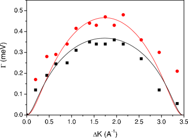
Figure 1: FWHM as a function of the parallel momentum transfer for Na diffusion on Cu(001) along the $[100]$ direction at $T=300$ K. Experimental datacoverage1 are indicated with symbols, while the solid lines are the fitted curves, obtained by applying Eq. (18). Two different values of the coverage are considered: $\theta_{1}=0.028$ (black) and $\theta_{2}=0.078$ (red).

Kramers’ turnover theory provides a two-parameter description of the diffusion process through the FWHM of the Q-peak versus the parallel momentum transfer. As seen in the preceding Section, these two parameters are the spatial diffusion rate and the energy loss. This treatment suits particularly well in fitting procedures applied to experimental data and/or numerical Langevin-type results due to the closed analytical expressions that are involved. Very good estimates of rates, diffusion coefficients and jump distributions are obtained when the barrier for diffusion exceeds the thermal energy and finite barrier corrections are also included. In Fig. 1, experimentalcoverage1 (symbols) and numerically fitted (solid lines) FWHM are plotted as a function of the parallel momentum transfer $\Delta K$ for Na diffusion on Cu(001) along the $[100]$ direction at $T=300$ K. Two different coverages are considered: $\theta_{1}=0.028$ (black squares/line) and $\theta_{2}=0.078$ (red circles/line). Fittings have been carried out using Eq. (18). The fitted values obtained for the spacial diffusion rate are $\Gamma_{sd}^{(1)}=0.250$ meV and $\Gamma_{sd}^{(2)}=0.238$ meV, and for the energy loss, $\delta_{1}=1.29$ and $\delta_{2}=1.97$. The broadening of the Q-peak with coverage is quite well reproduced by Eq. (18). Even more, as is clearly seen from Eq. (16), the diffusion coefficient decreases with the coverage (as shown previously in Ref. ruth3, ) and the energy loss increases with the coverage or friction according to Eq. (11).

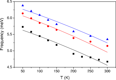
Figure 2: T-mode frequency as a function of the surface temperature for Na diffusion on Cu(001) along the direction $[100]$. Experimental datacoverage2 are indicated with symbols, while the solid lines are the fitted curves, obtained by applying Eq. (20). Three different values of the coverage are considered: $\theta_{1}=0.028$ (black), $\theta_{2}=0.078$ (red) and $\theta_{3}=0.125$ (blue).

The T-mode peak position and its FWHM are plotted in Figs. 2 and 3, respectively, as a function of the surface temperature and for three coverages: $\theta_{1}=0.028$ (black), $\theta_{2}=0.078$ (red) and $\theta_{3}=0.125$ (blue). In Fig. 2, the best fitted curves (solid lines) with respect to the corresponding experimental datacoverage2 (symbols) for the T-mode peak positions have been obtained from Eq. (20). The corresponding frequencies obtained when Eq. (20) is applied are: $\omega_{0}^{(1)}=2.13\times 10^{-4}$, $\omega_{0}^{(2)}=2.3\times 10^{-4}$, and $\omega_{0}^{(3)}=2.4\times 10^{-4}$, all given in atomic units (the nominal value being $2.20\times 10^{-4}$ a.u.). With the coverage, the T-mode frequency shifts towards higher values. After the definition of the effective frequency in Eq. (20), it should display the opposite trend with the coverage since a higher friction coefficient is required in the ISA model. However, the changes on $\omega_{0}$ are so small (less than 10$\%$) that we can not rule out small changes in the mean force potential. On the other hand, the best fitted values found for the anharmonicity constants (also through Eq. (20)) are $K_{4}^{(1)}=-6.17\times 10^{-14}$, $K_{4}^{(2)}=-8.05\times 10^{-14}$, and $K_{4}^{(3)}=-9.25\times 10^{-14}$, also in atomic units. For a cosine potential, $K_{4}$ is negative and therefore the anharmonicity produces a red shift with a linear temperature dependence.raul3 The agreement with the surface temperature is fairly good when second-order corrections in the anharmonicity are included. The different $\omega_{0}$ and $K_{4}$ values are slightly modified due to coverage, thus indicating a modification of the barrier/well and anharmonicity due to increasing amount of adsorbates, respectively. In general, in the presence of only one bath, the new system plus bath frequencies are renormalized due to the surface friction or coupling with the substrate.eli5 This renormalization takes into account the sum over all harmonic oscillators of the bath. In the two bath scenario, the corresponding renormalization has an extra sum coming from the adsorbates. Finally, Fig. 3 remains as a prediction since no experimental information is available about FWHM of the T-mode peaks. However, what is well-known from experiments is that the T-mode peak broadens with the coverage, which is theoretically predicted by Eq. (21).

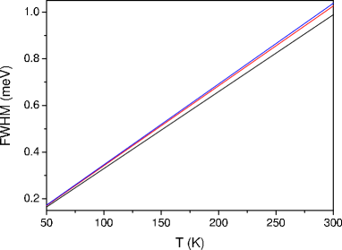
Figure 3: T-mode FWHM as a function of the surface temperature for Na diffusion on Cu(001) along the direction $[100]$. The solid lines have been obtained by means of Eq. (21) and using the values arisen from the fittings displayed in Fig. 2. Three different values of the coverage are considered: $\theta_{1}=0.028$ (black), $\theta_{2}=0.078$ (red) and $\theta_{3}=0.125$ (blue).

IV Conclusions

The main physical consequences of the approach presented here are that, on average, the tagged adparticle is seen as a diffusing particle among adsorbates which modify effective barriers and wells leading to the renormalization of frequencies as showed from a normal mode analysis.eli1 ; eli2 The corresponding renormalized frequencies have been reported for the one-bath model elsewhere.eli2 A straightforward generalization of the effective frequencies can be done for the two-bath model. In particular, this new approach could provide a theoretical framework to better interpret the coverage dependence of tunneling diffusion experimentszhu within a quantum Markovian formalism.ruth5 Many times, in surface diffusion LMD simulations surface barriers are only changed with the coverage in order to reproduce experimental data, keeping the corresponding frequencies fixed.

- (1) F. Hofmann and J.P. Toennies, Chem. Rev. 96, 1307 (1996).
- (2) S. Miret-Artés and E. Pollak, J. Phys.: Condens. Matter 17, S4133 (2005).
- (3) A.P. Jardine, H. Hedgeland, G. Alexandrowicz, W. Allison, and J. Ellis, Prog. Surf. Sci. 84, 323 (2009).
- (4) B. Farago, Physica B 267-268, 270 (1999).
- (5) P. Fouquet, H. Hedgeland, A. Jardine, G. Alexandrowicz, W. Allison, and J. Ellis, Physica B 385-386, 269 (2006).
- (6) J.R. Manson and V. Celli, Phys. Rev. B 39, 3605 (1989).
- (7) A.P. Graham, F. Hofmann, J.P. Toennies, L.Y. Chen, and S.C. Ying, Phys. Rev. Lett. 78, 3900 (1997); ibid. Phys. Rev. B 56, 10567 (1997).
- (8) J. Ellis and J.P. Toennies, Phys. Rev. Lett. 70, 2118 (1993).
- (9) J. Ellis and J. P. Toennies, Surf. Sci. 317, 99 (1994).
- (10) A. Cucchetti and S.C. Ying, Phys. Rev. B 60, 11110 (1999).
- (11) J. Ellis, A.P. Graham, F. Hofmann, and J.P. Toennies, Phys. Rev. B 63, 195408 (2001).
- (12) A.P. Graham and J.P. Toennies, Phys. Rev. B 56, 15378 (1997).
- (13) A. Cucchetti and S.C. Ying, Phys. Rev. B 54, 3300 (1996).
- (14) V.B. Magalinskii, Sov. Phys. JETP 9 (1959) 1381.
- (15) A.O. Caldeira and A.J. Leggett, Phys. Rev. Lett. 46, 211 (1981); ibid. Ann. Phys. 149, 374 (1983).
- (16) E. Cortés, B.J. West, and K. Lindenberg, J. Chem. Phys. 82, 2708 (1985).
- (17) H. Grabert, U. Weiss, and P. Hänggi, Phys. Rev. Lett. 52, 2193 (1984).
- (18) E. Pollak, Phys. Rev. A 33, 4244 (1986).
- (19) E. Pollak, J. Chem. Phys. 85, 865 (1986).
- (20) V.I. Mel’nikov and S.V. Meshkov, J. Chem. Phys. 85, 1018 (1986); V.I. Mel’nikov, Phys. Rep. 209, 1 (1991).
- (21) E. Pollak, H. Grabert, and P. Hänggi, J. Chem. Phys. 91, 4073 (1989)
- (22) I. Rips and E. Pollak, Phys. Rev. A 41, 5366 (1990).
- (23) A.M. Levine, M. Shapiro, and E. Pollak, J. Chem. Phys. 88, 1959 (1988).
- (24) R. Martínez-Casado, J.L. Vega, A.S. Sanz, and S. Miret-Artés, Phys. Rev. Lett. 98 216102 (2007).
- (25) R. Martínez-Casado, J.L. Vega, A.S. Sanz, and S. Miret-Artés, J. Phys.: Condens. Matter 19, 305002 (2007).
- (26) R. Martínez-Casado, J.L. Vega, A.S. Sanz, and S.Miret-Artés, Phys. Rev. B 77, 115414 (2008).
- (27) R. Martínez-Casado, J.L. Vega, G. Rojas-Lorenzo, A.S. Sanz, and S.Miret-Artés, “Linear response theory of activated surface diffusion with interacting adsorbates”, Chem. Phys.; e-print arXiv:cond-mat/0909.0719.
- (28) J.L. Vega, R. Guantes, and S. Miret-Artés, Phys. Chem. Chem. Phys. 4, 4985 (2002)
- (29) R. Guantes, J.L. Vega, S. Miret-Artés, and E. Pollak, J. Chem. Phys. 119, 2780 (2003)
- (30) R. Guantes, J.L. Vega, S. Miret-Artés, and E. Pollak, J. Chem. Phys. 120, 10768 (2004).
- (31) A.P. Graham, J.P. Toennies, and G. Benedek, Surf. Sci. 556, L143 (2004).
- (32) L. van Hove, Phys. Rev. 95, 249 (1954).
- (33) D.A. McQuarrie, Statistical Mechanics (Harper and Row, New York, 1976).
- (34) J.P. Hansen and I.R. McDonald, Theory of simple liquids (Academic Press, London, 1986).
- (35) H.A. Kramers, Physica (Utrecht) 7, 284 (1940).
- (36) P. Hänggi, P. Talkner, and M. Borkovec, Rev. Mod. Phys. 62, 251 (1990).
- (37) Y. Georgievskii and E. Pollak, Phys. Rev. E 49, 5098 (1994); Y. Georgievskii, M. A. Kozhushner, and E. Pollak, J. Chem. Phys. 102, 6908 (1995).
- (38) R. Martínez-Casado, J.L. Vega, A.S. Sanz, and S. Miret-Artés, Phys. Rev. E 75, 051128 (2007).
- (39) R.F. Grote, and J.T. Hynes, J. Chem. Phys. 73, 2715 (1980).
- (40) C.T. Chudley and R.J. Elliott, Proc. Phys. Soc. 57, 353 (1961).
- (41) A. Wong, A. Lee, and X.D. Zhu, Phys. Rev. B 51, 4418 (1995); G.X. Cao, E. Nabighina, and X.D. Zhu, Phys. Rev. Lett. 79, 3696 (1997).
- (42) R. Martínez-Casado, A.S. Sanz, and S. Miret-Artés, J. Chem. Phys. 129, 184704 (2008).