Hydrodynamic View of Wave-Packet Interference: Quantum Caves

Abstract

Wave-packet interference is investigated within the complex quantum Hamilton-Jacobi formalism using a hydrodynamic description. Quantum interference leads to the formation of the topological structure of quantum caves in space-time Argand plots. These caves consist of the vortical and stagnation tubes originating from the isosurfaces of the amplitude of the wave function and its first derivative. Complex quantum trajectories display counterclockwise helical wrapping around the stagnation tubes and hyperbolic deflection near the vortical tubes. The string of alternating stagnation and vortical tubes is sufficient to generate divergent trajectories. Moreover, the average wrapping time for trajectories and the rotational rate of the nodal line in the complex plane can be used to define the lifetime for interference features.

One of the most fundamental but intriguing microscopic effects is quantum interference, the observable feature arising from the coherent superposition of quantum probability amplitudes. Quantum interference is involved in a very wide range of experiments arising from myriad applications. Just to mention some of them, there are superconducting quantum interference devices scalapino , coherent control of chemical reactions paul , atom and molecular interferometry berman (including Bose-Einstein condensates pritchard ), or Talbot/Talbot-Lau interferometry with relatively heavy particles (e.g., Na atoms chapman2 and Bose-Einstein condensates deng ). However, despite all this experimental and theoretical work, very little attention beyond the implications of the superposition principle has been devoted to understanding quantum interference at a more fundamental level angel-jpa .

In this Letter, we focus on the hydrodynamical interpretation madelung ; wyatt-bk of experiments of this type by introducing complex quantum trajectories originating as characteristics of the solutions of the complex quantum Hamilton-Jacobi equation CQHJE1 ; CQHJE2 ; CQHJE3 ; CQHJE4 ; CQHJE5 ; CQHJE6 . As recently shown Tannor , interference effects on the real axis may be described in terms of the superposition of amplitudes carried by approximate (low-order) complex quantum trajectories. Unfolding of the dynamics from real space into the complex plane yields unexpected and surprising features, including what we term quantum caves. These caves are topological structures developed around curves in complex coordinate space where the total wave function and its first derivative are zero (nodes and stagnation points, respectively). Quantum caves are then displayed in 3D Argand plots (the third dimension being time), where vortical and stagnation tubes form around nodal and stagnation curves (which arise from the time-evolution of nodes and stagnation points, respectively), displaying analogies to the stalactites and stalagmites of real geological caves.

The equation of motion for complex quantum trajectories arises after substituting the complex-valued wave function in the form $\Psi(x,t)=\exp[iS(x,t)/\hbar]$ into the time-dependent Schrödinger equation. This yields the complex-valued quantum Hamilton-Jacobi equation

$$-\frac{\partial S}{\partial t}=\frac{1}{2m}\left(\frac{\partial S}{\partial x}\right)^{2}+V(x)+\frac{\hbar}{2mi}\frac{\partial^{2}S}{\partial x^{2}},$$ (1)

where $S(x,t)$ is the complex action and the last term is the complex quantum potential, $Q(x,t)$. For the system studied here, no external interaction potential is assumed (i.e., $V=0$). Quantum trajectories are then developed from the guidance condition $p(x,t)=\partial S(x,t)/\partial x$, which defines the quantum momentum function (QMF). By analytical continuation, the $x$ variable is extended to the complex plane through the $z=x+iy$ complex variable (time remains real-valued) and complex quantum trajectories are determined from $p(z,t)=\partial S(z,t)/\partial z=(\hbar/i)\partial\ln\Psi(z,t)/\partial z$. Two kinds of singularities are especially relevant: (i) nodes of the wave function, which correspond to poles of the QMF, and (ii) stagnation points chia-polya , which occur where the QMF is zero and correspond to points where the first derivative of the wave function is also zero. In addition, caustics are related to free wave-packet propagation angel .

To illustrate the formation of vortical and stagnation tubes and quantum caves, we consider the head-on collision of two one-dimensional Gaussian wave packets angel-jpa ; angel . Despite its simplicity, this analytical problem is a representative of other more complicated, realistic processes characterized by interference. This process can be described by the total wave function, $\Psi(x,t)=\psi_{L}(x,t)+\psi_{R}(x,t)$ ($L$/$R$ denotes left/right), which is analytically continued to the complex plane to give $\Psi(z,t)$. Each partial wave is represented by a free Gaussian wave packet,

$$\psi(x,t)=A_{t}\ \!e^{-(x-x_{t})^{2}/4\sigma_{t}\sigma_{0}+ip(x-x_{t})/\hbar+iEt/\hbar},$$ (2)

where, for each component, $A_{t}=(2\pi\sigma_{t}^{2})^{-1/4}$ and the complex time-dependent spreading is given by $\sigma_{t}=\sigma_{0}(1+i\hbar t/2m\sigma_{0}^{2})$ with the initial spreading $\sigma_{0}$. Due to the free motion, $x_{t}=x_{0}+vt$ ($v=p/m$ is the propagation velocity) and $E=p^{2}/2m$. We also consider the case where the relative propagation velocity is larger than the wave packet spreading rate, $\hbar/2m\sigma_{0}$ angel-jpa . From now on, all quantities will be given in atomic units ($\hbar=m=1$).

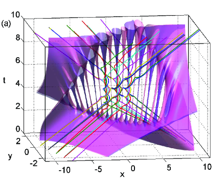
Figure 1: Quantum caves for head-on collision of two Gaussian wave packets. These caves are formed with the isosurfaces $|\Psi(z,t)|=0.053$ (pink/lighter gray sheets) and $|\partial\Psi(z,t)/\partial z|=0.106$ (violet/darker gray sheets). The complex quantum trajectories launched from two branches of the isochrone reach the real axis at $t=5$.

The following initial conditions are used: $x_{0L}=-10=-x_{0R}$, $v_{L}=2=-v_{R}$ and $\sigma_{0}=\sqrt{2}$, and maximal interference occurs at $t=5$ in real space. In Fig. 1, complex quantum trajectories together with the isosurfaces $|\Psi(z,t)|=0.053$ (pink/lighter gray sheets) and $|\partial\Psi(z,t)/\partial z|=0.106$ (violet/darker gray sheets) from $t=0$ to $t=10$ are shown in a 3D Argand plot. Around nodes and stagnation points, tubular shapes develop (pink/lighter gray and violet/darker gray tubes, respectively), which alternate with each other and whose centers correspond to vortical and stagnation curves, respectively. The sharp features and well defined vertical tubes observed in Fig. 1, reminiscent of stalactites and stalagmites, lead us to call these plots quantum caves. Interference leads to the formation of quantum caves and produces this topological structure.

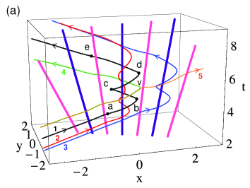
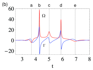
Figure 2: (a) Trajectories 1, 2, 3 and 4 launched from the isochrone which arrive on the real axis at $t=5$ display hyperbolic deflection around the vortical curves (pink/light gray) and helical wrapping around the stagnation curves (violet/dark gray). Trajectories 4 and 5 diverge at position “V” near the vortical curve. (b) Divergence and vorticity of the QMF along trajectory 1.

As seen in Fig. 1 and, in more detail, in Fig. 2(a), the complex trajectories display counterclockwise helical wrapping around the stagnation tubes, while they are hyperbolically deflected or “repelled” when they approach the vortical tubes enclosing the QMF poles. This intricate motion depicts the probability density flow around the vortical and stagnation tubes. Trajectories launched from different initial positions may wrap around the same stagnation curve and remain trapped for a certain time interval. As time proceeds, these trajectories separate from the stagnation curves in analogy to the decay of a resonant state. Therefore, the whole process shows long-range correlation among trajectories arising from different starting points.

The QMF can be viewed as a vector field in the complex plane, $p=p_{x}+ip_{y}$, and we can compute its divergence and vorticity along a complex quantum trajectory, which describe the local expansion or contraction and rotation of the quantum fluid, respectively. By the Cauchy-Riemann equations, the first derivative of the QMF becomes $\partial p/\partial z=(\Gamma+i\Omega)/2$, where $\Gamma=\vec{\nabla}\cdot\vec{p}=\partial p_{x}/\partial x+\partial p_{y}/\partial y$ is the divergence of the QMF and $\Omega=|\vec{\nabla}\times\vec{p}\,|=(\partial p_{y}/\partial x-\partial p_{x}/\partial y)$ is the vorticity. Moreover, the complex quantum potential in Eq. (1) can be expressed in terms of divergence and vorticity by

$$Q(z,t)=\frac{\hbar}{2mi}\frac{\partial p}{\partial z}=\frac{\hbar}{4mi}\left(\Gamma+i\Omega\right).$$ (3)

Figure 2(a) shows trajectories 1, 2, 3 and 4 launched from the isochrone which arrive on the real axis at $t=5$ (maximal interference), and Fig. 2(b) presents the time evolution of the divergence and vorticity of the QMF along trajectory 1. When the particle approaches the vortical curve at position $a$, it experiences a repulsive force provided by the pole of the QMF and the trajectory displays hyperbolic deflection. As shown in Fig. 2(b), $\Gamma$ and $\Omega$ display the first sudden spike. Then, this particle is trapped by the stagnation curve between two vortical curves. When the trajectory approaches turning points ($b$, $c$ and $d$), the particle’s velocity undergoes rapid changes and this produces sharp fluctuations in $\Gamma$ and $\Omega$. From Eq. (3), the quantum potential is larger near these positions. Finally, as the particle departs from the stagnation curve, it experiences a repulsive force provided by the pole and the trajectory displays hyperbolic deflection at position $e$. The whole process indicates important dynamical activity, which is lacking within the real-valued version of this problem (where no divergence or vorticity can be defined).

The wrapping time for a specific trajectory can be defined by the interval between the first and last minimum of $\Omega$, and the positive vorticity within this time interval describes the counterclockwise twist of the trajectory. The sign of $\Gamma$ indicates the local expansion or contraction of the quantum fluid when it approaches or leaves a turning point, respectively. Within this time interval, the particle obviously feels the presence of stagnation points and nodes, and the trajectory displays the interference dynamics. From Fig. 2(b), the wrapping process lasts from $t\approx 3.7$ to $t\approx 6.9$. In addition, trajectories 1 and 2 wrap around the same stagnation curve with different wrapping times and numbers of loops. The wrapping time around a stagnation curve is determined by $\Gamma$ and $\Omega$, which are used to characterize the turbulent flow. Thus, the average wrapping time for those trajectories reaching the real axis at the time of maximal interference can be used to define the “life-time” for the interference process observed on the real axis.

Trajectories 2 and 3 start from the isochrone with the initial separation $\Delta z_{0}\approx 0.3$, wrap around different stagnation curves, and then end with the separation at $t=10$ $\Delta z\approx 0.8$. These two trajectories avoid the vortical curve and this greatly increases the separation between them. This behavior is consistent with what one observes when looking at the quantum flow in real space: the trajectory distribution is sparse near nodes of the wave function and dense between two consecutive nodes. In addition, trajectories 4 and 5 start with slightly different initial positions, $\Delta z_{0}=0.01$, and they suddenly separate at position “V” near the vortical curve. This leads to the continuously increasing separation between them and a positive Lyapunov exponent, analogous to the case reported in real space CQHJE4 . The alternating structure for the vortical and stagnation tubes (similar to that for the nodal point–X-point complex in Bohmian mechanics in 2D real space) thus leads to divergent trajectories and may generate chaos Efthymiopoulos .

Time-dependent nodal positions in the complex plane can be determined analytically by solving the equation $\Psi(z,t)=0$, which renders

$$z_{n}(t)=\frac{i\pi\left(n+1/2\right)}{\left[imv/\hbar-\left(x_{0}-vt\right)/\left(2\sigma_{0}\sigma_{t}\right)\right]},$$ (4)

where $n=0,\pm 1,\pm 2,\ldots$ Splitting this expression into its real and imaginary parts, $z_{n}(t)=x_{n}(t)+iy_{n}(t)$, yields the analytical expression for the angle of the nodal line with the positive real axis, $\theta(t)=\tan^{-1}\left[y_{n}(t)/x_{n}(t)\right]$, (which is independent of $n$), and this describes the time evolution of the nodal line. In addition, the time evolution of the $n$th node is given by $y_{n}=(2mv\sigma_{0}^{2}/\hbar x_{0})x_{n}-(2n+1)(\pi\sigma_{0}^{2}/x_{0})$.

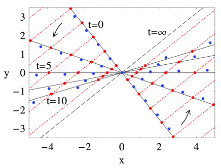
Figure 3: Evolution of the nodal line at $t=0,2.5,5,7.5,10$ (black solid lines) and $t=\infty$ (black dashed line); the arrows indicate the rotation direction. Nodes and stagnation points are denoted by dots; nodal trajectories are shown as dotted lines passing through the nodal points.

Figure 3 shows the time-dependent string of stagnation points and nodes and nodal trajectories in the complex plane. At $t=0$, these two wave packets are far away from each other; however, their tails interfere in the complex plane. This contributes to the string of stagnation points and nodes, and the initial angle of the nodal line (which is perpendicular to nodal trajectories) is $\theta_{0}=\tan^{-1}(-\hbar x_{0}/2mv\sigma_{0}^{2})=-51.34^{\circ}$. Then, the nodal line rotates counterclockwise and crosses the real axis at $t=5$, where the total wave function displays maximal interference. At this time, $y_{n}=0$ and we recover the expression for the positions of nodes, $x_{n}=(n+1/2)\lambda/2$ ($\lambda=h/mv$). After $t=5$, these two wave packets start to separate, and the nodal line continues to rotate counterclockwise away from the real axis. However, these two wave packets still interfere with each other in the complex plane. When $t$ tends to infinity, the angle of the nodal line approaches $\theta_{\infty}=\tan^{-1}(2mv\sigma_{0}^{2}/\hbar x_{0})=38.66^{\circ}$ and this line becomes parallel to nodal trajectories. The nodal line rotates counterclockwise angel from $\theta_{0}$ to a limiting value $\theta_{\infty}$ with an angular displacement $\Delta\theta=\theta_{\infty}-\theta_{0}=\pi/2$, and its intersections with nodal trajectories determine the positions of nodes. In addition, the distance between stagnation points and nodes increases with time. In particular, if both wave packets are initially very far apart ($x_{0}\to\infty$) but move with a finite velocity $v$, or they are separated by an arbitrary finite distance with $v=0$, then the nodal line will end up aligned with the real axis. Interference features are observed on the real axis only when the nodal line is near the real axis. For the case shown in Fig. 3, this occurs between about $\theta(3.52)=-10^{\circ}$ and $\theta(7.32)=10^{\circ}$, so that the “lifetime” for the interference features is about $\Delta t=3.8$. Therefore, the lifetime of interference features observed on the real axis is determined by the rotation rate of the nodal line in the complex plane, and this rate $d\theta(t)/dt$ decays monotonically to zero as $t\to\infty$.

The complex quantum trajectory method provides an insightful alternative to the traditional analysis of quantum interference phenomena in real space. In Bohmian mechanics, when two or more real coordinates are involved, quantum vortices form around nodes in the wave function and streamlines surrounding the vortex core form approximately circular loops Hirschfelder ; sanz-jcp . The interference of two wave packets in one real coordinate leads to the formation of nodal structure, but quantum trajectories close to nodes forming at the maximal interference time do not display vortical dynamics angel . The quantum potential near these nodes forces these trajectories to avoid these regions and to exhibit laminar flow in space-time plots. In contrast, complex quantum trajectories displaying helical wrapping and hyperbolic deflection undergo turbulent flow in the complex plane. This counterclockwise circulation of trajectories launched from different positions around the same stagnation tubes can be viewed as a resonance process in the sense that during interference some trajectories keep circulating around the tubes for finite times and then escape as time progresses. On the other hand, in conventional quantum mechanics, the interference pattern transiently observed on the real axis is attributed to constructive and destructive interference between components of the total wave function. In contrast, within the complex quantum trajectory formalism, two counter-propagating wave packets are always interfering with each other in the complex plane. This leads to a persistent pattern of nodes and stagnation points which is a signature of the “quantum coherence” demonstrating the connection between both wave packets before or after interference fringes are observed on the real axis. The interference features observed on the real axis are connected to the rotational dynamics of the nodal line in the complex plane. Therefore, the average wrapping time for trajectories and the rotation rate of the nodal line in the complex plane provide two methods to define the interference lifetime observed on the real axis. This analysis demonstrates that the complex quantum trajectory method provides a novel perspective and leads to new insights for analyzing and interpreting quantum mechanical problems. Finally, similar conclusions are drawn when the spreading velocity of the wave packets is greater than their propagation velocity.

C.-C. Chou and R. E. Wyatt thank the Robert Welch Foundation for the financial support of this research; A.S. Sanz and S. Miret-Artés acknowledge the Ministerio de Ciencia e Innovación (Spain) for financial support under Project FIS2007-62006. A. S. Sanz also acknowledges the Consejo Superior de Investigaciones Científicas for a JAE-Doc contract.

References

- (1) D.J. Scalapino, The Theory of Josephson Tunneling, in Tunneling Phenomena in Solids, eds. E. Burstein and S. Lundqvist (Plenum Press, New York, 1969) pp. 477-518.
- (2) P.W. Brumer and M. Shapiro, Principles of the Quantum Control of Molecular Processes (Wiley-Interscience, Hoboken, New York, 2003).
- (3) P.R. Berman (ed.), Atom Interferometry (Academic Press, San Diego, 1997).
- (4) Y. Shin et al., Phys. Rev. Lett. 92, 050405 (2004); M. Zhang et al., Phys. Rev. Lett. 97, 070403 (2006); L.S. Cederbaum et al., Phys. Rev. Lett. 98, 110405 (2007).
- (5) M.S. Chapman et al., Phys. Rev. A 51, R14 (1995).
- (6) L. Deng et al., Phys. Rev. Lett. 83, 5407 (1999).
- (7) A.S. Sanz and S. Miret-Artés, J. Phys. A 41, 435303 (2008).
- (8) E. Madelung, Z. Phys. 40, 322 (1926).
- (9) R.E. Wyatt, Quantum Dynamics with Trajectories (Springer, New York, 2005).
- (10) W. Pauli, it Die allgemeine Prinzipien der Wellenmechanick, Handbuch der Physik, 24, Part 1, 2nd ed, eds. H. Geiger and K. Scheel (Springer-Verlag, Berlin, 1933).
- (11) A.S. Sanz, F. Borondo and S. Miret-Artés, J. Phys.: Condens. Matter 14, 6109 (2002).
- (12) M.V. John, Found. Phys. Lett. 15, 329 (2002); Ann. Phys. 324, 220 (2009).
- (13) R. Guantes, A.S. Sanz, J. Margalef-Roig and S. Miret-Artés, Surf. Sci. Rep. 53, 199 (2004).
- (14) C.-D. Yang, Ann. Phys. 319, 444 (2005).
- (15) D. Tannor, Introduction to Quantum Mechanics (University Science Books, Sausalito, CA, 2007).
- (16) Y. Goldfarb, I. Degani and D.J. Tannor, J. Chem. Phys. 125, 231103 (2006); A.S. Sanz and S. Miret-Artés, J. Chem. Phys. 127, 197101 (2007); Y. Goldfarb, I. Degani and D.J. Tannor, J. Chem. Phys. 127, 197102 (2007); Y. Goldfarb and D.J. Tannor, J. Chem. Phys. 127, 161101 (2007).
- (17) C.-C. Chou and R.E. Wyatt, J. Chem. Phys. 128, 234106 (2008); 129, 124113 (2008).
- (18) A.S. Sanz and S. Miret-Artés, Chem. Phys. Lett. 458, 239 (2008).
- (19) C. Efthymiopoulos, C. Kalapotharakos and G. Contopoulos, J. Phys. A 40, 12945 (2007).
- (20) J.O. Hirschfelder, A.C. Christoph and W.E. Palke, J. Chem. Phys. 61, 5435 (1974); J.O. Hirschfelder, C.J. Goebel and L.W. Bruch, J. Chem. Phys. 61, 5456 (1974).
- (21) A.S. Sanz, F. Borondo and S. Miret-Artés, J. Chem. Phys. 120, 8794 (2004); Phys. Rev. B 69, 115413 (2004).