Nonlinear Ramsey interferometry with the Rosen-Zener pulses on a two-component Bose-Einstein condensate

Abstract

We propose a feasible scheme to realize nonlinear Ramsey interferometry with a two-component Bose-Einstein condensate, where the nonlinearity arises from the interaction between coherent atoms. In our scheme, two Rosen-Zener pulses are separated by an intermediate holding period of variable duration and through varying the holding period we have observed nice Ramsey interference patterns in the time domain. In contrast to the standard Ramsey fringes our nonlinear Ramsey patterns display diversiform structures ascribed to the interplay of the nonlinearity and asymmetry. In particular, we find that the frequency of the nonlinear Ramsey fringes exactly reflects the strength of nonlinearity as well as the asymmetry of system. Our finding suggests a potential application of the nonlinear Ramsey interferometry in calibrating the atomic parameters such as scattering length and energy spectrum.

I Introduction

The technique of Ramsey interferometry with separated oscillating fields was first proposed to investigate the molecular beam resonance Ram1950 . The key feature of the observed Ramsey pattern in the frequency domain is that the width of the central peak is determined by the inverse of the time taken by the particle to cross the intermediate drift region PRA76(2007)two-level . Indeed, the Ramsey interference experiments can be operated either in the time domain with temporally separated pulses and fixed particle or in the space domain with spatially separated fields and moving particle PRA75(2007)two-frequency . The Ramsey’s interferometric method provides the basis of atomic fountain clocks that now serve as time standards PRL82(1999) ; PRL85(2000) and stimulates the rapid advancement in the field of precision measurements in atomic physics. Since applying the laser cooling techniques to trapped atoms, the atom interferometers with cold atoms have been used to measure rotation rotation1 , gravitational acceleration rotation2 ; acceleration , atomic fine-structure constant PRL70(1993) , atomic recoil frequency PRA67(2003) , and atomic scattering properties PRL92(2004) , to name only a few.

On the other hand, the experimental realization of the Bose-Einstein condensate (BEC) in a dilute atomic gas BECfind1 ; BECfind2 brings a fascinating opportunity for the purpose of precision measurement due to the very slow atoms and changes the prospects of frequency standards entirely. Recently, Ramsey fringes between atoms and molecules in time domain have been observed by using trapped BEC of ⁸⁵Rb atoms AMRam1 in experiment. This offers the possibility of precise measurement of binding energy of the molecular state in BEC AMRam2 ; AMRam3 .

With the development of atom interferometry techniques, researchers are seeking to exploit new interferometric methods using trapped BEC InBECs ; chli1 . With the emergence of the nonlinear interaction between the coherent ultracold atoms, the BECs show marvelous nonlinear tunneling and interference properties that are distinguished from the traditional quantum systems. Motivated by our recent study on nonlinear Rosen-Zener (RZ) transition Ye , in this paper we construct a nonlinear Ramsey interferometer with applying a sequence of two identical nonlinear RZ tunneling processes (i.e., RZ pulses). The RZ model was first proposed to study the spin-flip of two-level atoms interacting with a rotating magnetic field to explain the double Stern-Gerlach experiments RZT . Differing from the Landau-Zener model LZT , RZ model has set the energy difference between two modes as a constant whereas the coupling strength is time dependent. In our interferometry scheme, two RZ pulses are separated by a intermediate holding period of variable duration and through varying the holding period we have observed diversiform Ramsey interference patterns in contrast to the standard Ramsey fringes. Using a simple nonlinear two-mode model, we thoroughly investigate the physics underlying the interference patterns both numerically and analytically. We find that the frequency of the nonlinear Ramsey fringes exactly reflects the strength of nonlinearity as well as the asymmetry of system. This observation suggests an potential application in calibrating the atom parameters such as scattering length and energy spectrum via measuring the frequency of Ramsey fringes.

Our paper is organized as follows. In Sec. II, we present our nonlinear Ramsey interferometer and demonstrate diversiform interference patterns. In Sec. III, we make detailed theoretical analysis on the nonlinear Ramsey interferometry. In the sudden limit and adiabatic limit, we have derived analytically the frequencies of the fringes in time domain and their dependence of the atomic parameters. Sec. IV is our discussions and applications, where we also extend our discussions to the double-well BEC systems.

II Nonlinear Ramsey interferometry

II.1 Interferometer scheme

We consider that a condensate, for example, ⁸⁷Rb atoms in a magnetic trap are driven by a microwave coupling into a linear superposition of two different hyperfine states, i.e., $F=1,m_{F}=-1$ and $F=2,m_{F}=+1$. A near resonant pulsed radiation laser field is used to couple the two internal states. The total density and mean phase remain constant during the condensate evolution. Within the standard rotating-wave approximation, for any one pulse the Hamiltonian describing the transition between the two internal states can be read ($\hbar=1$)

$$\hat{H}=-\frac{\gamma}{2}(\hat{a}^{\dagger}\hat{a}-\hat{b}^{\dagger}\hat{b})-\frac{c}{4}(\hat{a}^{\dagger}\hat{a}-\hat{b}^{\dagger}\hat{b})^{2}+\frac{v}{2}(\hat{a}^{\dagger}\hat{b}+\hat{b}^{\dagger}\hat{a}),$$ (1)

where $\hat{a}$ ($\hat{b}$) and $\hat{a}^{\dagger}$ ($\hat{b}^{\dagger}$) are boson annihilation and creation operators for two components, respectively. $\gamma=-\delta+(4N\pi\hbar^{2}/m)(a_{11}-a_{22})\eta$ is the energy difference between two states characterizing the asymmetry of the system, $c=(2\pi\hbar^{2}/m)(a_{11}+a_{22}-2a_{12})\eta$ is the nonlinear strength describing atomic interactions, and $v$ denotes the coupling strength which is proportional to the intensity of near-resonant laser field. $\delta$ is the detuning of lasers from resonance, $a_{ij}$ is the $s-$wave scattering amplitude of hyperfine species $i$ and $j$, $\eta$ is a constant of order 1 independent of the hyperfine index, relating to an integral of equilibrium condensate wave function RMP73(2001) , $N$ is the atom number, and $m$ is the mass of atom.

In the limit of large particle number, the operators in the above field equations could be replaced by the complex numbers, we thus obtain following mean-field equations that describe the evolution of the above two-component BEC system effectively,

$$i{d\over dt}\left(\begin{array}[]{c}a\\ b\end{array}\right)=H(v)\left(\begin{array}[]{c}a\\ b\end{array}\right),$$ (2)

with the Hamiltonian

$$H(v)=\left(\begin{array}[]{cc}\frac{\gamma}{2}+\frac{c}{2}(|b|^{2}-|a|^{2})&\frac{v}{2}\\ \frac{v}{2}&-\frac{\gamma}{2}-\frac{c}{2}(|b|^{2}-|a|^{2})\\ \end{array}\right),$$ (3)

where $a$ and $b$ denote the amplitudes of probabilities for two components and the total probability $|a|^{2}+|b|^{2}=1$.

Using the above two-component BEC system we are capable to realize a nonlinear Ramsey interferometer, in which the nonlinearity represents the interparticle interaction. The main structure of our nonlinear Ramsey interferometer is illustrated by Fig. 1, in which the variation of the coupling strength is governed by two Rosen-Zener pulses of the form:

$$v(t)=\left\{\begin{array}[]{ll}0,&t<0;\\ v_{0}\sin^{2}(\frac{\pi t}{T}),&t\in[0,T];\\ 0,&t\in(T,T+\tau);\\ v_{0}\sin^{2}[\frac{\pi(t-T-\tau)}{T}],&t\in[T+\tau,2T+\tau];\\ 0,&t>2T+\tau.\end{array}\right.$$ (4)

The above RZ pulses are characterized by following parameters: $v_{0}$ is the maximum strength of the coupling, $T$ is the scanning period of RZ pulse, and $\tau$ is an alterable time interval between two pulses.

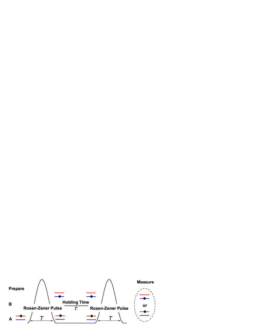
Figure 1: (Color online) Schematic plot of nonlinear Ramsey interferometer with two-component trapped BEC in time domain, starting with a RZ pulse, addition of a holding period, ending with another RZ pulse.

This scheme is analogous to a normal Ramsey interferometer while the Ramsey pulses at the beginning and the end of the sequence that couple the two components and redistribute the populations on each component are replaced by so called nonlinear RZ tunneling process Ye . The two tunneling processes are separated by a holding period. During the holding period, there is no coupling between the two components and the BEC on each component will evolve independently and only acquire different additional phases. In the course of the simulative experiments, the system is prepared in one internal state initially, the final populations of atoms in each state are recorded when the second pulse turns off. The measurements are repeated with variable time interval $\tau$. The final populations are sensitive to the phase difference built up between two components during the intermediate period, as a result, the Ramsey fringes pattern is expected to emerge in time domain.

II.2 Ramsey fringe patterns

The nonlinear Schrödinger equations (2) that govern the temporal evolution of the two-component BEC system are solved numerically using standard Runge-Kutta 4-5th algorithm. We set the initial condition $(a,b)=(1,0)$, and take the maximum coupling strength as the energy scale, namely, $v_{0}=1$. The Ramsey fringe patterns have been obtained by recording the final transition probability $|b|^{2}$ versus the holding time $\tau$.

We begin our numerical simulations with the linear case of $c=0$ for $T=20$. Figs. 2(a) and 2(d) shows the variation of the transition probability for symmetric case ($\gamma=0$) and asymmetric case ($\gamma=0.1$), respectively. Actually Eq. (2) can be solved analytically for the symmetric case, the solution is $\sin^{2}(v_{0}T/2)$ which depends on the scanning period $T$ only. The numerical result in Fig. 2(a) coincides with the analytic prediction that the transition probability keeps a constant $0.29596$. For the asymmetric system the standard Ramsey fringes pattern of typical sinusoidal is shown as Fig. 2(d).

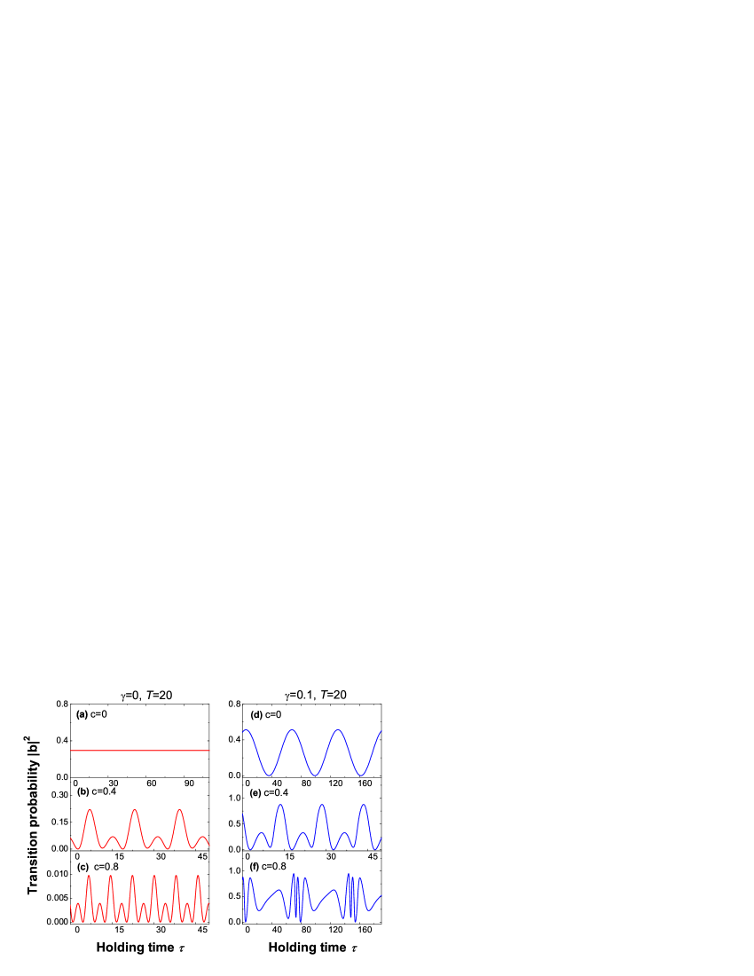
Figure 2: (Color online) Ramsey fringe patterns for symmetric case (left column) and asymmetric case (right column) under different nonlinear parameters with $T=20$. (a) and (d) $c=0$, (b) and (e) $c=0.4$, (c) and (f) $c=0.8$.

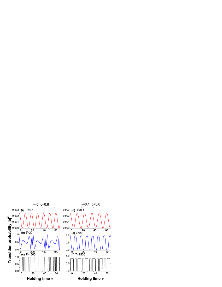
Figure 3: (Color online) Ramsey fringe patterns for symmetric case (left column) and asymmetric case (right column) under different scanning periods with $c=0.6$. (a) and (d) $T=0.1$, (b) and (e) $T=20$, (c) and (f) $T=1500$.

With the emergence of nonlinearity, the Ramsey fringes pattern distinctly deviates from that of linear case due to the dramatic changes of the transition dynamics. In this case the system (2) is no longer analytically solvable. Our numerical simulations for different nonlinear parameters and various scanning periods of the RZ pulse have been displayed in Figs. 2 and 3, respectively. Fig. 2 show that both nonlinearity and symmetry can affect the pattern and the frequency of Ramsey fringes significantly. By analyzing the results in Figs. 2 and 3 we find that the Ramsey fringes pattern includes perfect sinusoidal or cosinoidal oscillation [see Figs. 2(d), 3(a) and 3(d)], trigonometric oscillation with multiple period [see Figs. 2(b), 2(c), 2(e), 2(f), 3(b), and 3(e)], and rectangular oscillation [see Figs. 3(c) and 3(f)]. Furthermore, we also find that the sinusoidal Ramsey pattern only exists in the linear case ($c=0$) and the rapid scanning case ($T=0.1$) while the rectangular oscillation only emerges in the very slow scanning case ($T=1500$). These diversiform interference patterns are distinguished from the normal Ramsey fringes of sinusoidal or cosinoidal forms and are obviously evoked by the nonlinear atomic interaction.

III Theoretical Analysis and Extended Numerical Simulation

In this section we will present thorough analysis on these striking interference patterns. In practical experiments, in contrast to the oscillating amplitudes and shapes of the fringe patterns, the frequencies of the patterns are of more interest and could be recorded with relatively high resolution and contrast, therefore we focus our theoretical analysis on the frequency property extracted from the Ramsey interference patterns through the Fourier transformation (FT). We find that the frequencies of patterns that are dramatically modulated by the interplay of nonlinearity and symmetry and contain many information about the intrinsic properties of the BEC system.

Through investigating the nonlinear Ramsey patterns presented above we see the time scale of the period of the RZ pulse plays an important role in forming the striking patterns. So our following discussions are divided into two limit cases, i.e., sudden limit and adiabatic limit. In the former case, the time scale of the RZ pulse is fast compared to the intrinsic motion of the system that is characterized by the frequency $v_{0}$, while the adiabatic limit refers to the case that the RZ pulse is much slower than intrinsic motion of the system.

III.1 Sudden limit case, i.e., $T\ll 2\pi/v_{0}$.

In our simulation, we choose the scanning period of the RZ pulse $T$ as $0.1$ that is much smaller than the intrinsic period of the system $2\pi/v_{0}$ . For both symmetric and asymmetric cases we extract the angular frequency information of the Ramsey fringes through making the FT analysis on the data. The results have been demonstrated in Fig. 4(a). A perfect linear increase relation between the angular frequencies of Ramsey fringes and nonlinear parameters is shown for symmetric case [see the solid squares in Fig. 4(a)]. For the asymmetric case, the frequency decreases linearly and then increases linearly as the nonlinear strength increases [see the solid triangles in Fig. 4(a)]. The dip to zero at $c=\gamma=0.1$ is clearly seen in the asymmetric system.

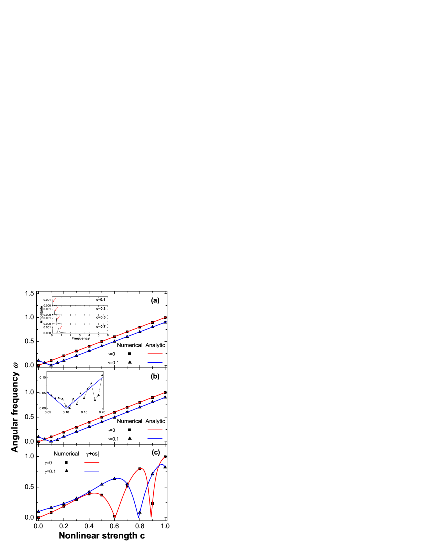
Figure 4: (Color online) Angular frequency $\omega$ of Ramsey fringes as a function of the nonlinear strength $c$. The numerical results well agree with analytic predictions. (a) sudden limit case, the inset displays the frequency spectrum of Ramsey fringes obtained from Fourier transformation for different $c$ with $\gamma=0$ (red arrows refer to the numerical results plotted in main plot). (b) adiabatic limit case, the inset demonstrates the details for $\gamma=0.1$ with $c$ from 0.05 to 0.2. (c) general situation.

Now we explain the above numerical results through some analytic deduction. Considering that the transition probability from one state to the other state is small enough in the sudden limit, thus we can use the perturbation method to analyze the system (2). We introduce the following variable transformation

$$a=a^{\prime}\exp\left[-i\int_{0}^{t}\left(\frac{\gamma}{2}+\frac{c}{2}(|b|^{2}-|a|^{2})\right)dt\right],$$ (5)

$$b=b^{\prime}\exp\left[i\int_{0}^{t}\left(\frac{\gamma}{2}+\frac{c}{2}(|b|^{2}-|a|^{2})\right)dt\right].$$ (6)

Following this transformation, we transform the diagonal terms in the Hamiltonian (3) away and obtain the first-order amplitude of $b(T)$ which yields $b(T)=\int_{0}^{t}\frac{v_{0}}{2}\sin^{2}(\frac{\pi t}{T})\mathrm{e}^{i(c-\gamma)t}dt|_{t=T}$. Finally, the transition probability after the first RZ pulse is given by

$$|b(T)|^{2}=\frac{2\pi^{4}v_{0}^{2}[1-\cos(\Omega T)]}{\Omega^{2}(4\pi^{2}-\Omega^{2}T^{2})^{2}},$$ (7)

where $\Omega=c-\gamma$. For convenience, we introduce a phase shift $\phi(\tau)$ to describe the different phase accumulations between two components during the holding period. Considering that two components evolve independently during this period, we get $\phi(\tau)=|\gamma+cs|\tau$ from Eq. (2), where $s=|b(T)|^{2}-|a(T)|^{2}$ denotes the population difference between two components when the first pulse has been turned off. This phase shift is proportional to the holding time. Obviously, the angular frequency of the Ramsey fringes is expected to be

$$\omega=|\gamma+cs|.$$ (8)

This result implies that the frequency of Ramsey fringes is entirely determined by the population difference $s$ and the parameters $\gamma$ and $c$. Substituting Eq. (7) into the above formula, we obtain the angular frequency of Ramsey fringes in the form

$$\omega=\left|\frac{4cv_{0}^{2}\pi^{4}[1-\cos(\Omega T)]}{\Omega^{2}[4\pi^{2}-(\Omega T)^{2}]^{2}}-\Omega\right|.$$ (9)

The above analytical predictions are compared with our numerical results in Fig. 4(a) and a perfect agreement is shown. Indeed, under the sudden limit assumption, the term $\Omega T$ in Eq. (9) is a small quantity, the numerator of the first term on the right-hand side of Eq. (9) is close to zero due to $\cos(\Omega T)\rightarrow 1$. When $T\rightarrow 0$, one can safely neglect the first term on the right-hand of Eq. (9), then the frequency is proportional to the parameter $|\Omega|$.

III.2 Adiabatic limit case, i.e., $T\gg 2\pi/v_{0}$.

In order to ensure the scanning period long enough, we set $T$ as $1500$ in calculation. In contrast to the linear case and the sudden limit case, an important phenomenon in this case is found that the FT on Ramsey fringes reveals multiple frequency components, namely, $\omega=n\omega_{0}$, where $\omega_{0}$ is the fundamental frequency (i.e., basic or first frequency) of the fringes, $n$ is a positive integer. We interpret this in terms of the interplay between nonlinearity ascribed to the interatomic interaction and the coupling energy from the external laser field. Fig. 4(b) only illustrates the fundamental frequencies of Ramsey fringes for different nonlinear parameters.

The results in this case are very similar to that in sudden limit case. However, a novel phenomenon is that there is a irregular fluctuation in near $c=\gamma$ region [see the inset in Fig. 4(b)]. We guess the adiabatic assumption is violated in this region. To confirm this argument, we trace the population difference $s$ after the first RZ pulse with nonlinear parameter increasing. The results are presented in Fig. 5, we see that a irregular oscillation of $s$ occurs in the region where $|\gamma-c|$ is very small as well. With the nonlinear parameter increasing from 0.25 to 1, $s$ will jump between two points $+1$ and $-1$ in symmetric case. However, for asymmetric system, when $c>0.35$, the value of $s$ will jump between $-1$ and another unknown point. This is a more intriguing quantum phenomenon and more essentially physical reasons need further detailed study.

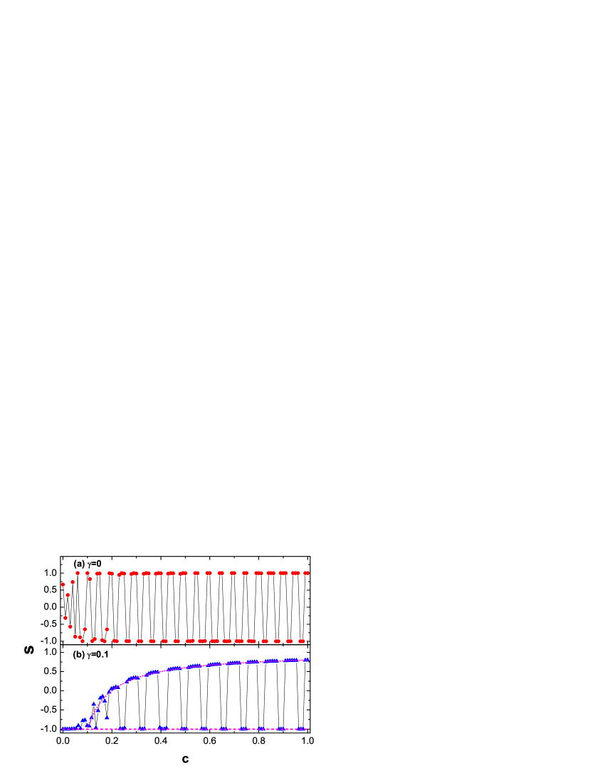
Figure 5: (Color online) The population difference $s$ versus nonlinear parameters from 0 to 1 for symmetric case (red circles) and asymmetric case (blue triangles) with $T=1500$. The dotted and dashed lines refer to theoretical prediction from Eq. (14).

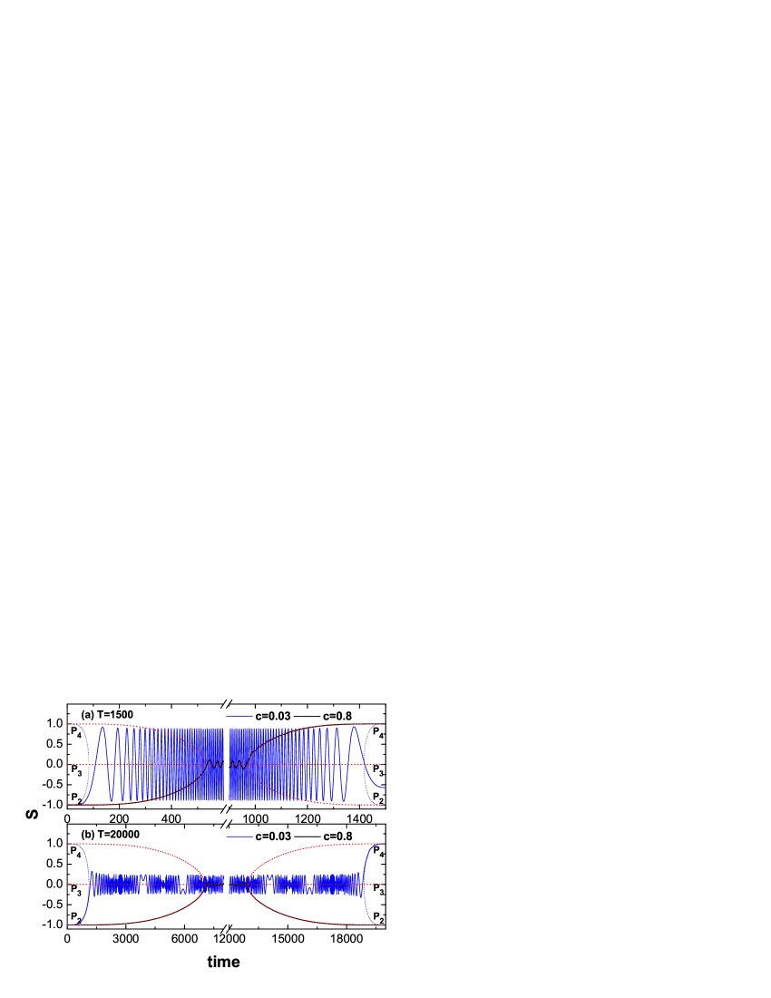
Figure 6: (Color online) Comparison between the dynamical evolution (solid line) and the adiabatic evolution (dotted line) of fixed points for symmetric case with different $T$: (a) $1500$, (b) $20000$. Blue line and black line refer to $c=0.03$ and $c=0.8$, respectively. Blue dotted line and red dotted line show the corresponding adiabatic evolution obtained from Eq. (11).

In order to explain the above peculiar phenomena, under the mean-field approximation, following Ref. clasicalH , we introduce the relative phase $\theta=\theta_{b}-\theta_{a}$ and the population difference $s=|b|^{2}-|a|^{2}$ as two canonical conjugate variables, then we can obtain an effective classical Hamiltonian

$$\mathcal{H}=-(\gamma+{c\over 2}s)s+v\sqrt{1-s^{2}}\cos\theta.$$ (10)

This classical Hamiltonian can describe completely the dynamic properties of system (2) clasicalH . The adiabatic evolution of the quantum eigenstates can be evaluated by tracing the shift of the classical fixed points in phase space when the parameter $v$ varies in time slowly fixedpoint . According to Refs. Ye ; prefu , for symmetric system we get the classical fixed points on line $\theta^{\ast}=\pi$,

$$s^{\ast}=\left\{\begin{array}[]{ll}0,&c/v<1;\\ 0,\pm\sqrt{1-(v/c)^{2}},&c/v>1.\end{array}\right.$$ (11)

We show the evolution of fixed point $s^{\ast}=-1$ ($P_{2}$) in Fig. 6. The three fixed points in Eq. (11) are characterized by $P_{3}$, $P_{4}$ and $P_{2}$, respectively. One saddle point $P_{3}$ ($s^{\ast}=0$) and two elliptic points $P_{2}$ and $P_{4}$ correspond to one unstable state and two stable states. For $c=0.8$, a good agreement between dynamical evolution and adiabatic trajectory of $P_{2}$ is shown both for $T=1500$ and $T=20000$. However, for $c=0.03$, the evolution of fixed point $P_{2}$ shows a clear deviation from the adiabatic trajectory given by Eq. (11) at $T=1500$ [see Fig. 6(a)] while the fixed point can follow the adiabatic evolution at $T=20000$ [see Fig. 6(b)]. The phenomena indicate that the adiabatic condition cannot be satisfied for $c=0.03$ where occurs the irregular fluctuation at $T=1500$ in Fig. 5. Therefore, we give the adiabatic condition as follows:

$$T\gg\mathrm{Max}\left[\frac{2\pi}{|\gamma-c|},\frac{2\pi}{v_{0}}\right].$$ (12)

Under this condition, so long as $\gamma\neq c$, the system will evolve adiabatically if the scanning period is long enough even for the small nonlinear parameters prefu . This can successfully explain the novel fluctuation in Figs. 4(b) and 5. Accordingly, we trace the fixed point $P_{2}$ in asymmetric case (see Fig. 7) using same parameter $T$ as in Fig. 6. The similar feature that good adiabatic evolution for $c=0.8$ and nonadiabatic evolution for $c=0.18$ where is in the close vicinity of the zero-energy resonance ($\gamma=c$) with $T=1500$ is observed. In addition, another interesting phenomenon is also find, despite the evolution process of the fixed point is not clear, there are two final states of adiabatic evolution to be choose for the fixed point [see Fig. 7(b) and Fig. 5(b)] for asymmetric case. We will interpret it by some deeply physical analysis below.

Figure 7: (Color online) Evolution of fixed points for asymmetric case under different $T$: (a) $1500$, (b) $20000$.

For the adiabatic limit case, the energy of system both for symmetric and asymmetric cases is no longer conservative during the entire evolution process, however at the beginning and end of the evolution the corresponding energies of the system keep the same value,

$$\mathcal{H}(s=-1,t=0)=\mathcal{H}(s^{\ast},t=T).$$ (13)

In our scheme, both for $t=0$ and $t=T$, the coupling parameter $v=0$. Thus we can get the final state of system from Eqs. (10) and (13)

$$s^{\ast}=\left\{\begin{array}[]{ll}-1,&\gamma>c;\\ -1,1-2\gamma/c,&0<\gamma<c.\end{array}\right.$$ (14)

This result implies that,at the end of the adiabatic evolution, the system has two states to choose when $c>\gamma$ for this case, one choice is back to the initial state $s^{\ast}=-1$ and the other choice is located on another state of the identical energy with the initial state $s^{\ast}=1-2\gamma/c$. However the latter choice restricts the population to $|b|^{2}=\gamma/c$, in other words, the quantum tunneling for asymmetric case require the atom number on another state must be not more than $N\gamma/c$ ($N$ is the total number of atoms). We use the above analysis to check our numerical results in Fig. 5(b) and a good agreement is shown. According to this analytic prediction, in adiabatic limit case, the final value of $s$ should be $-0.11$ or $-1$ for $c=0.18$ and $0.75$ or $-1$ for $c=0.8$ in Fig. 7, these results strongly support our numerical results.

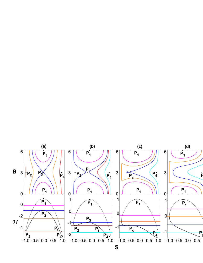
Figure 8: (Color online) Evolution of the phase space motions as $c/v$ changes adiabatically (upper panel) with $\gamma=0.5$. (a) $c/v=10$, (b) $c/v=3$, (c) $c/v=2.0897$, (d) $c/v=1$. The lower panel is the corresponding energy curve for $\theta=0$ (black thin line) and $\pi$ (black heavy line).

In order to provide a simple intuitive understand of this adiabatic evolution process, we study the evolution of fixed points in phase space as shown in Fig. 8. $P_{1}$, $P_{2}$ and $P_{4}$ in the upper panel of Fig. 8 are all elliptic points corresponding to the local maximum ($P_{1}$) and minimum ($P_{2}$ and $P_{4}$) of the classical Hamiltonian indicated in the lower panel of Fig. 8, respectively. We see the quantum transition between two states can be explained by a collision between two fixed points. When $c/v$ decreases from $10$ to $1$, the fixed point $P_{2}$ will collide with the unstable saddle point $P_{3}$ at $P_{c}$ and disappear subsequently, as shown in Figs. 8$(a)\rightarrow(b)\rightarrow(c)\rightarrow(d)$. The condition of the collision is given by Ref. fixedpoint , namely,

$$v=(c^{2/3}-\gamma^{2/3})^{3/2}.$$ (15)

For the case with $\gamma=0.5$, the collision occurs at $c/v=2.0897$ [see Fig. 8(c)]. However, when $c/v$ increases from 1 to 10 again, the state of system will choose either stable fixed point $P_{2}$ or a stable trajectory $P_{t}$ which is of identical energy with $P_{2}$ to follow after the dynamical bifurcation at $P_{c}$ [see Figs. 8$(c)\rightarrow(b)\rightarrow(a)$]. This is a peculiar and intriguing phenomenon that only emerges in asymmetric system. Following the above analysis, we can obtain the analytic expression of fundamental frequency of Ramsey fringes in adiabatic limit from Eqs. (9) and (14)

$$\omega=|\gamma-c|.$$ (16)

The results show a perfect linear relation both for symmetric and asymmetric cases and are consistent with our numerical results [see 4(b)].

III.3 General situation

In this subsection, we turn to study the general case where the scanning period of RZ pulse is of the same order with $2\pi/v_{0}$, i.e., $T=20$. We will show the population difference $s$ can greatly affect the frequency of Ramsey fringes in this case. Similarly, we show the fundamental frequencies of Ramsey fringes in Fig. 4(c). The comparison between numerical results and theoretical prediction $|\gamma+cs|$ show a good agreement. In Fig. 4(c), the perfect linear relation has been completely broken, and three zero-frequency points emerge: one in asymmetric case and two in symmetric case. The physics behind this is that the balance between energy difference characterized by $\gamma$ and the interatomic interaction energy controlled by the nonlinear term $cs$. When the nonlinear parameters satisfy the balance condition $\gamma=-cs$, there will occur zero-energy resonance or the zero-frequency points.

To confirm this argument, we trace the population difference with the nonlinear parameter increasing. The results show that, for symmetric case when two components are of identical populations, the Ramsey fringes vanish and the zero-frequency points emerge. The concrete process of evolution of system in general case is not clear due to the complex quantum transition behaviors.

III.4 The dependence of frequency of $\gamma$

In this part, we briefly investigate the case which sets the nonlinear parameter as a constant and takes $\gamma$ as an alterable quantity.

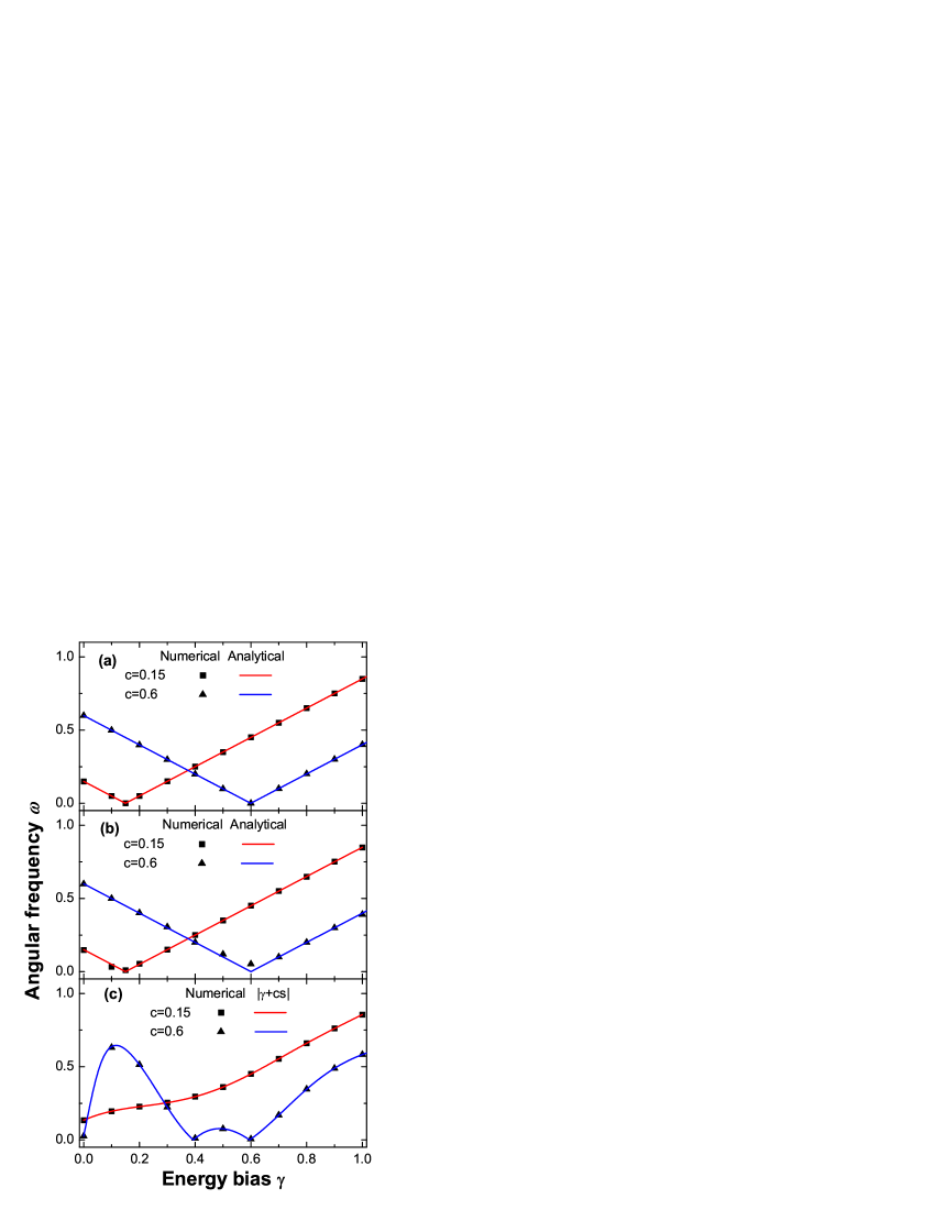
Figure 9: (Color online) The angular frequency of Ramsey fringes versus the energy difference $\gamma$ for different cases. (a) sudden limit; (b) adiabatic limit; (c) general situation.

Following the previous analysis, the fundamental frequency of Ramsey fringes is also expected to be $\omega=|\gamma+cs|$. Fig. 9 shows the fundamental frequencies of Ramsey fringes versus energy difference $\gamma$ for different scanning periods. We have used the same parameter $T$ as in Fig. 4, and Figs. 9(a), (b), and (c) refer to the sudden limit, the adiabatic limit and the general case, respectively.

By analyzing these plots, we see that, there is a common property for three cases, zero-frequency points emerge when the nonlinear parameter equals to the energy difference for large nonlinear parameter $c=0.6$. However, for small nonlinear parameter $c=0.15$, there does not occur zero-frequency points in general case while zero-frequency points emerge in sudden limit and adiabatic limit cases. Here, we restrict our consideration to $\gamma>0$ and $c>0$. In fact, we find the zero-frequency point in general case occurs at $\gamma=-0.118$ for $c=0.15$, and the zero-frequency point in general case is more than one.

In particular, the similar irregular fluctuation in the region around $\gamma=c$ has been found in Fig. 9(b). The smaller the nonlinear parameter is, the larger the amplitude of irregular oscillation shows. This implies that in the region around $\gamma/c=1$, the system does not satisfy the adiabatic condition (12). If the scanning period is long enough, the novel fluctuation in Fig. 9(b) will become smooth prefu .

IV Discussions and Applications

In summary, based on the quantum Rosen-Zener tunneling process, we propose a feasible scheme to realize nonlinear Ramsey interferometry with a two-component Bose-Einstein condensate, where the nonlinearity arises from the interaction between coherent atoms. In our scheme, two RZ pulses are separated by an intermediate holding period of variable duration and through varying the holding period we have observed nice Ramsey fringe patterns in time domain. In contrast to the standard Ramsey fringes our nonlinear Ramsey patterns display diversiform structures due to the interplay of the nonlinearity and asymmetry. In particular, we find that the frequency of the nonlinear Ramsey fringes exactly reflects the strength of nonlinearity as well as the asymmetry of system. Our study suggests that our interferometry scheme can be used to measure the atomic parameters such as scattering length, atom number and energy spectrum through measuring the frequency of nonlinear Ramsey interference fringe patterns.

Our nonlinear Ramsey interferometer scheme can also be realized using the BECs with a double-well potential. This BEC system, under the mean-field approximation, is described by following Gross-Pitaevskii equation (GPE)

$$i\hbar\frac{\partial\Psi(r,t)}{\partial t}=\left[-\frac{\hbar^{2}}{2m}\nabla^{2}+V(r)+U_{0}|\Psi(r,t)|^{2}\right]\Psi(r,t),$$ (17)

where $U_{0}=4\pi\hbar^{2}a_{s}N/m$ with $m$ the atomic mass and $a_{s}$ the $s-$wave scattering length of the atoms. The wave function can be described by a superposition of two states that localize in each well separately as smerzi $\Psi(r,t)=\psi_{1}(t)\phi_{1}(r)+\psi_{2}(t)\phi_{2}(r).$ The spatial wave function $\phi_{i}(r)$ ($i=1,2$) which describe the condensate in each well can be expressed in terms of symmetric and antisymmetric stationary eigenstates of GPE, and these two wave functions satisfy the orthogonality condition $\int\phi_{1}(r)\phi_{2}(r)dr=0$ and normalized condition $\int|\phi_{i}(r)|^{2}dr=1$. Consider the weakly linked BEC, the dynamic behavior of system can be described by Schrödinger equation with the Hamiltonian as follows:

$$H=\left(\begin{array}[]{cc}\epsilon^{0}_{1}+c_{1}|\psi_{1}|^{2}&K\\ K&\epsilon^{0}_{2}+c_{2}|\psi_{2}|^{2}\\ \end{array}\right),$$ (18)

where $\epsilon^{0}_{i}=\int[\frac{\hbar^{2}}{2m}|\nabla\phi_{i}|^{2}+|\phi_{i}|^{2}V(r)]dr$ ($i=1,2$) is the zero-point energy in each well. $\Delta\epsilon=\epsilon_{1}-\epsilon_{2}$ is the energy bias. $c_{i}=U_{0}\int|\phi_{i}|^{4}dr$ denotes the atomic self-interaction. $K=\int[\frac{\hbar^{2}}{2m}(\nabla\phi_{1}\nabla\phi_{2})+\phi_{1}V(r)\phi_{2}]dr$ stands for the the amplitude of the coupling between two wells.

For example, consider one dimension case, we can express the potential of our system as $V({x})=\frac{1}{2}m\omega x^{2}+v_{0}\mathrm{e}^{-{x^{2}}/{2d}}+fx$, $d$ is the double-well separation in $x$ direction. This optical double-well potential can be created by superimposing a blue-detuned laser beam upon the center of the magnetic trap 2well , the difference of the zero-point energy between two wells or trap asymmetry characterized by $f$ can be bringed by a magnetic field, a gravity field or light shifts gravity . The atomic interaction $c$ can be adjusted flexibly by Feshbach resonance, and the barrier height $K$ can be effectively controlled by adjusting the intensity of the blue-detuned laser beam.

V Acknowledgments

This work is supported by National Natural Science Foundation of China (No.10725521,10604009,10875098), the National Fundamental Research Programme of China under Grant No. 2006CB921400, 2007CB814800.

References

- (1) N. F. Ramsey, Phys. Rev. 78, 695 (1950).
- (2) S. V. Mousavi, A. del Campo, I. Lizuain, and J. G. Muga, Phys. Rev. A 76, 033607 (2007).
- (3) D. Seidel and J. G. Muga, Phys. Rev. A 75, 023811 (2007).
- (4) G. Santarelli et al., Phys. Rev. Lett. 82, 4619 (1999).
- (5) C. Fertig and K. Gibble, Phys. Rev. Lett. 85, 1622 (2000).
- (6) T. L. Gustavson, P. Bouyer, and M. A. Kasevich, Phys. Rev. Lett. 78, 2046 (1997).
- (7) B. Dubetsky and M. A. Kasevich, Phys. Rev. A 74, 023615 (2006).
- (8) A. Peters et al., Nature (London) 400, 849 (1999).
- (9) D. S. Weiss et al., Phys. Rev. Lett. 70, 2706 (1993).
- (10) M. Weel and A. Kumarakrishnan, Phys. Rev. A 67, 061602(R) (2003).
- (11) A. Widera et al., Phys. Rev. Lett.92, 160406-1 (2004).
- (12) M. H. Anderson, J. R. Ensher, M. R. Matthews, C. E. Wieman, and E. A. Cornell, Science 269, 198 (1995); K. B. Davis et al., Phys. Rev. Lett. 75, 3969 (1995); C. C. Bradley et al., ibid. 75, 1687 (1995).
- (13) M. R. Andrews, C. G. Townsend, H.-J. Miesner, D. S. Durfee, D. M. Kurn, and W. Ketterle, Science 275, 637 (1997).
- (14) E. A. Donley, N. R. Claussen, S. T. Thompson, and C. E. Wieman, Nature (London) 417, 529 (2002).
- (15) N. R. Claussen, S. J. J. M. F. Kokkelmans, S. T. Thompson, E. A. Donley, E. Hodby, and C. E. Wieman, Phys. Rev. A 67, 060701 (2003).
- (16) Krzysztof Góral, Thorsten Köhler, and Keith Burnett, Phys. Rev. A 71, 023603 (2005).
- (17) T. Schumm et al., Nature Phys. 1, 57 (2005).
- (18) C. H. Lee, Phys. Rev. Lett. 97, 150402 (2006).
- (19) D. F. Ye, L. B. Fu, and J. Liu, Phys. Rev. A 77, 013402 (2008).
- (20) N. Rosen and C. Zener, Phys. Rev. 40, 502 (1932).
- (21) L. D. Landau, Phys. Z. Sowjetunion 2, 46 (1932); G. Zener, Proc. R. Soc. London, Ser. A 137, 696 (1932).
- (22) A. J. Leggett, 73, 307 (2001).
- (23) Jie Liu, Biao Wu and Qian Niu, Phys. Rev. Lett. 90, 170404 (2003).
- (24) Jie Liu, Li-bin Fu, Bi-Yiao Ou et al., Phys. Rev. A 66, 023404 (2002).
- (25) L. B. Fu, S. G. Chen, Phys. Rev. E 71, 016607 (2005).
- (26) A. Smerzi, S. Fantoni, S. Giovanazzi, and S. R. Shenoy, 79, Phys. Rev. Lett. 22, 4950 (1997); S. Raghavan, A. Smerzi, S. Fantoni, and S. R. Shenoy, Phys. Rev. A 59, 620 (1999).
- (27) M. R. Andrews et al., Science 275, 637 (1997).
- (28) B. V. Hall, S. Whitlock, R. Anderson, P. Hannaford, and A. I. Sidorov, Phys. Rev. Lett. 98, 030402 (2007).