A unified Monte Carlo treatment of gas-grain chemistry for large reaction networks. I. Testing validity of rate equations in molecular clouds

Abstract

In this study we demonstrate for the first time that the unified Monte Carlo approach can be applied to model gas-grain chemistry in large reaction networks. Specifically, we build a time-dependent gas-grain chemical model of the interstellar medium, involving about 6000 gas-phase and 200 grain surface reactions. This model is used to test the validity of the standard and modified rate equation methods in models of dense and translucent molecular clouds and to specify under which conditions the use of the stochastic approach is desirable.

Two cases are considered: (1) the surface mobility of all species is due to thermal hopping, (2) in addition to thermal hopping, temperature-independent quantum tunneling for H and H₂ is allowed. The physical conditions characteristic for the core and the outer region of TMC1 cloud are adopted. The gas-phase rate file RATE 06 together with an extended set of gas-grain and surface reactions is utilized.

We found that at temperatures 25–30 K gas-phase abundances of H₂O, NH₃, CO and many other gas-phase and surface species in the stochastic model differ from those in the deterministic models by more than an order of magnitude, at least, when tunneling is accounted for and/or diffusion energies are 3x lower than the binding energies. In this case, surface reactions, involving light species, proceed faster than accretion of the same species. In contrast, in the model without tunneling and with high binding energies, when the typical timescale of a surface recombination is greater than the timescale of accretion onto the grain, we obtain almost perfect agreement between results of Monte Carlo and deterministic calculations in the same temperature range. At lower temperatures ($\sim 10$ K) gaseous and, in particular, surface abundances of most important molecules are not much affected by stochastic processes.

1 Introduction

Chemical processes are discrete in nature, and it has been realized long time ago that their microphysically correct theoretical treatment should rest upon stochastic methods (Gillespie, 1976). While in cellular biology Monte Carlo simulations of chemical processes in cells are widespread, most models in astrochemistry are based on deterministic rate equation (RE) approach, which has been proved to be inaccurate for chemical processes on “cell-like” objects like dust grains and PAHs (Tielens & Hagen, 1982; Caselli et al., 1998; Herbst & Shematovich, 2003; Lipshtat & Biham, 2003; Stantcheva & Herbst, 2004). The concept of mass-action kinetics, which lies behind rate equations, being adequate for gas-phase reactions, is not appropriate in the case of small surface population (number of particles $\leq 1$ per grain). This situation is often the case in grain surface catalysis. Rates of surface reactions obtained through this approach may be strongly incorrect, leading to an improper estimation of timescales of fundamental processes, like H₂ formation, and significant errors in abundances of other species.

Up to now, a number of attempts have been made to assess the significance of stochastic effects for astrochemical simulations and to develop suitable numerical methods. In the context of astrochemistry first attempt to treat grain surface chemistry stochastically has been made by Tielens & Hagen (1982). In this study, equilibrium abundances of gas-phase species were used to obtain accretion rates and to calculate time-dependent populations of surface species through Monte Carlo approach. All surface species but H₂ were assumed to remain on the grain surfaces.

Subsequent attempts to account for the discrete nature of surface reactions can be divided into two categories. The first category encompasses different modifications to the rate equations for grain surface chemistry (Caselli et al., 1998, 2002; Stantcheva et al., 2001). The main idea behind these modifications is to restrict rates of diffusive surface reactions by accretion or desorption rates of reactants. Thus, the so–called accretion-limited regime is taken into account, when the rate of a particular surface reaction is determined by the flux of reactants accreting on a grain and not by their diffusion over the surface. For simple reacting systems, results obtained with this semi-empirical approach were found, at least, to be in closer agreement with Monte Carlo (MC) computations than the treatment by rate equations alone. However, the applicability of the modified rate equations (MRE) to large chemical networks has not been tested so far. Moreover, it is impossible to investigate purely stochastic effects, like bistability, with this technique, still purely deterministic in its nature (Le Bourlot et al., 1993; Shalabiea & Greenberg, 1995; Lee et al., 1998; Boger & Sternberg, 2006).

In the second category of studies the master equation is solved with different methods. Because the chemical master equation describes probabilities of a chemically reacting system to be in all possible states of its phase space and the number of these states grows exponentially with the number of species, their direct integration is only possible for extremely simple systems, consisting of a very few different components. Biham et al. (2001), Green et al. (2001) and Lipshtat et al. (2004) have performed a direct integration of the master equation to investigate H₂ formation. These studies demonstrated that in some cases this fundamental process cannot be adequately described with the rate equation approach. In Stantcheva et al. (2002), Caselli et al. (2002) and Stantcheva & Herbst (2003) direct integration of the master equation was applied to study the evolution of a simple H—O—CO surface chemical network and deuterium fractionation. Direct integration of the master equation in more complex networks of grain surface reactions is hampered by the lack of appropriate computing power. To the best of our knowledge, the only successful simulation of a more extended surface chemical network in astrochemistry, consisting of 19 reactions, with direct integration of the master equation was accomplished by Stantcheva & Herbst (2004).

A Monte Carlo approach based on continuous-time random-walk method has been developed by Chang et al. (2005) to model recombination of hydrogen atoms on interstellar grains. The advantage of this method is that it allows to model formation of H₂ and other molecules on surfaces of arbitrary roughness, which has later been demonstrated by Cuppen & Herbst (2007).

To relax computational requirements needed to solve the master equation, the moment equation approximation was suggested by Lipshtat & Biham (2003) and Barzel & Biham (2007). Currently, this is the most promising approach to efficient simulations of gas-grain systems with complex grain surface chemistry, because the moment equations can be easily combined with rate equations used to simulate gas-phase chemical processes. But, strictly speaking, the moment equations are an approximation and their validity should be verified by a comparison with exact methods.

The only feasible technique allowing us to obtain an exact solution to the master equation for complex chemically reacting systems is Monte Carlo method developed by Gillespie (1976). This approach is widely used in molecular biology for simulation of chemical processes in living cells and can also be applied to astrochemical problems. Gillespie’s Stochastic Simulation Algorithm (SSA) was first used in complex astrochemical networks by Charnley (1998), where SSA was applied to gas-phase chemistry only. Later a simple grain surface H—O—CO chemical model, similar to the one considered in Caselli et al. (1998), was developed by Charnley (2001). In this model, gas-phase abundances of species were assumed to be constant and desorption was neglected. No coupled gas-grain chemical model was studied.

The chemical master equation is usually considered as a method to model surface reactions. However, due to its universality, it can be used to model the gas-phase chemistry as well. The reason why the rate equations are so popular as a tool to study gas-phase chemistry in astronomical environments is the fact that they are easier to implement and much more computationally effective. However, if one uses the rate equations to model gas-phase chemistry and some stochastic approach to model surface chemistry one has to find a way to match the two very different computational techniques. The first study in which a Monte Carlo treatment of grain surface chemistry was coupled to time-dependent gas-phase chemistry is Chang et al. (2007). In this paper iterative technique is utilized to combine very different Monte Carlo and rate equations approaches. Calculations are performed for the time interval of $2\cdot 10^{5}$ years and a relatively simple H—O—CO surface network consisting of 12 reactions is used.

Even though remarkable progress has been made to develop stochastic approaches to astrochemistry, up to now there are no studies in which a stochastic treatment of a complex grain surface chemical network is fully coupled to time-dependent gas-phase chemistry. The situation gets less complicated when the same method is used for both gas-phase and surface chemistry. In this paper, for the first time, we present a “complete” time-dependent chemical gas-grain model, calculated with Monte Carlo approach. We solve the master equation with a Monte Carlo technique, using it as a single method to treat gas-phase reactions, surface reactions, and gas-grain exchange processes simultaneously. The gas-phase chemical network includes more than 6000 reactions while surface network consists of more than 200 reactions.This Monte Carlo model is used to test the validity of rate equations and modified rate equations for a range of physical conditions, typical of diffuse and dense clouds. So far, no comparison of RE and MRE techniques against rigorous stochastic approach over a wide range of physical conditions, typical for astrophysical objects, has been made.

There is clear observational evidence that interstellar grains have complex mineral composition and may have either amorphous or crystalline structure. In general, it is believed that interstellar dust particles are made of olivine-like silicates and some form of amorphous carbon or even graphite (Draine & Lee, 1984). The location on a surface which may be occupied by an accreted molecule is commonly referred to as a surface site. The density of sites and binding energies for specific species strongly depend on the dust material and its structure. Binding energies $E_{\rm b}$, that is, potential barriers between adjacent sites, have been assumed by Hasegawa et al. (1992) to be roughly 0.3 of corresponding desorption energies $E_{\rm D}$. In Pirronello et al. (1997a, b, 1999), Katz et al. (1999) and Perets et al. (2005) experimental results on the H₂ formation, the ratio of diffusion energy to desorption energy, $E_{\rm b}/E_{\rm D}$, was found to be close to 0.77 for H atoms. This ratio determines the surface mobility of species and is of utter importance for estimating surface reaction rates.

Another factor defining rates of reactions involving H and H₂ (and their isotopologues) is related to the possibility of their tunneling. Non-thermal quantum tunneling of these species allows them to scan grain surface and find a reacting partner quickly. This mechanism has been suggested as an explanation of efficient H₂ formation in the ISM. Later analysis of the cited experimental results has lead Katz et al. (1999) to the conclusion that tunneling does not happen. The absence of tunneling implies lower mobility, so that surface processes are essentially reduced to accretion and desorption. However, this conclusion turned out to be not the final one. In other studies (e.g. Cazaux & Tielens, 2004) alternative explanations of these experiments have been proposed and some shortcomings of the theoretical analysis performed in Katz et al. (1999) have been found. So, up to now the question of presence or absence of tunneling effects on grain surfaces is not settled, and the $E_{\rm b}/E_{\rm D}$ ratio is not well constrained. With this in mind, two different models of grain surface reactions are considered: (1) the surface mobility of all species is caused by thermal hopping only with high $E_{\rm b}/E_{\rm D}$ ratio equal to 0.77, (2) temperature-independent quantum tunneling for H and H₂ is included in addition to thermal hopping with low $E_{\rm b}/E_{\rm D}$ ratio equal to 0.3.

The organization of the paper is as follows. In Section 2 we describe physical conditions adopted in simulations and chemical model used. Section 3 contains basics of stochastic reaction kinetics and detailed description of the Monte Carlo code used for simulations. In Section 4 the validity of rate equations and modified rate equations is checked against Monte Carlo method. First, global agreement between methods is investigated. Then, some interesting species are discussed separately. In Section 5 a discussion is presented. Section 6 contains the conclusions.

2 Modeling

2.1 Physical conditions

In the present study, we consider grain surface reactions under physical conditions typical of irradiated translucent clouds, cold dark cores and infrared dark clouds. We consider temperatures $T$ between 10 and 50 K, densities $n(\rm H)$ between 200 and $2\cdot 10^{4}$ cm^-3 (three values of $n(\rm H)$ and five values of $T$), and visual extinctions of 0.2 mag at $n({\rm H})=200$ cm^-3, 2.0 mag at $n({\rm H})=2\cdot 10^{3}$ cm^-3 and 15 mag at $n({\rm H})=2\cdot 10^{4}$ cm^-3 (e.g., Snow & McCall, 2006; Hassel et al., 2008). This $A_{\rm v}$ roughly corresponds to the distance of order of 0.4–0.5 pc from the cloud boundary (at constant density). The cloud is illuminated by the mean interstellar diffuse UV field. The dust temperature is assumed to be equal to gas temperature. We do not study the earliest stage of the molecular cloud evolution, which is essentially the stage when atomic hydrogen is converted into hydrogen molecules. The chemical evolution is simulated assuming static physical conditions. While it is still a matter of debate how long does it take for a typical isolated cloud core to become gravitationally unstable and to start collapsing, we assume a short timescale of 1 Myr which seems to be appropriate for the TMC1 cloud (see e.g. Roberts et al., 2004; Semenov et al., 2004).

2.2 Chemical model

The chemical model is the same as described in Vasyunin et al. (2008). The gas-phase reactions and their rates are taken from the RATE 06 database, in which the effects of dipole-enhanced ion-neutral rates are taken into account (Woodall et al., 2007). All reactions with large negative activation barriers are excluded. The rates of photodissociation and photoionization of molecular species by interstellar UV photons are taken from van Dishoeck et al. (2006). The self- and mutual shielding of CO and H₂ against UV photodissociation are computed as described in van Zadelhoff et al. (2003) using pre-calculated factors from Tables 10 and 11 from Lee et al. (1996). Ionization and dissociation by cosmic ray particles are also considered, with a cosmic-ray ionization rate of $1.3\cdot 10^{-17}$ s^-1 (Spitzer & Tomasko, 1968).

The gas-grain interactions include accretion of neutral species onto dust grains, thermal and photodesorption of mantle materials, dissociative recombination of ions on charged grains and grain re-charging processes. The dust grains are uniform $0.1\,\mu$m spherical particles made of amorphous silicates of olivine stoichiometry (Semenov et al., 2003), with a dust-to-gas mass ratio of $1\%$. The sticking probability is 100%. Desorption energies $E_{\rm D}$ and surface reaction list are taken from Garrod & Herbst (2006).

The grain surface is assumed to be compact, with surface density of $2\cdot 10^{14}$ sites cm^-2, which gives $\approx 3\cdot 10^{5}$ sites per grain (Biham et al., 2001). We employ two models to calculate the rates of surface reactions (Table 1). In Model T (T for tunneling) the tunneling timescale for a light atom to overcome the potential barrier and migrate to another potential well is computed using Eq. (10) from Hasegawa et al. (1992), with the barrier thickness of 1Å. In Model H (H for hopping) we do not allow H and H₂ to scan surface sites by tunneling. The diffusion timescale for a molecule is calculated as the timescale of thermal hopping multiplied by the total number of surface site and is given by Eq. (2) and Eq. (4) from Hasegawa et al. (1992). The hopping rates are sensitive to the adopted values of diffusion energy, which are not well constrained. Thus, we consider low and high diffusion energies which are calculated from adopted desorption energies by multiplying them by factors of 0.3 (like in Hasegawa et al., 1992) (Model T) and 0.77 (Katz et al., 1999) (Model H), respectively. For all considered models, the total rate of a surface reaction is calculated as a sum of diffusion or tunneling rates divided by the grain number density and multiplied by the probability of reactions (100% for processes without activation energy).

Overall, our network consists of 422 gas-phase and 157 surface species made of 13 elements, and 6002 reactions including 216 surface reactions. As initial abundances, we utilize the “low metallicity” set of Lee et al. (1998), where abundances of heavy elements in the gas are assumed to be severely depleted. All hydrogen is molecular initially. The chemical evolution for 1 Myr in the classical deterministic approaches is computed with the fast “ALCHEMIC” code in which the modified rate equations are implemented according to Caselli et al. (1998). No further modification for reactions with activation energy barriers is used (see Caselli et al., 2002).

3 Stochastic reaction kinetics

3.1 Theoretical foundations

We consider a chemically reacting system which consists of $N$ different types of species {$S_{1}$ … $S_{N}$} and $M$ chemical reactions {$R_{1}$ … $R_{M}$} (Gillespie, 1976). All these species are contained in a constant volume $\Omega$, in which local thermal equilibrium is reached, so that the system is well mixed. We denote the number of species of type $i$ at time $t$ as $X_{i}(t)$. The ultimate goal is to determine the state vector $\vec{X}(t)=\{X_{1}(t)...X_{N}(t)\}$ of the system at any given time $t>t_{0}$, assuming certain initial conditions $\vec{X}(t_{0})=\vec{X}_{0}$.

Let us assume that each reaction $R_{j}$ retains properties of a Markov chain and can be considered as a set of independent instantaneous events. Each chemical reaction is described by two quantities, the discrete state vector $\vec{\nu}=\{\nu_{1j},...,\nu_{Nj}\}$ and the propensity function $a_{j}$. The components of the state vector $\nu_{ij}$ represent the net change in populations of the $i$th species due to the $j$th reaction. By definition, the propensity function

$$a_{j}(\vec{X})dt$$ (1)

is the probability for a reaction $R_{j}$ to occur in the volume $\Omega$ over the time interval $dt$. In analogy to the reaction rate in the rate equation approach, for a one-body reaction the propensity function $a_{j}$ can be expressed through rate constants and numbers of reactants as

$$a_{j}(\vec{X})=c_{j}x_{1}.$$ (2)

Here, $c_{j}$ is the rate constant of the $j$th reaction and $x_{1}$ is the absolute population of reagent. For a two-body heterogeneous reaction this expression changes as follows:

$$a_{j}(\vec{X})=c_{j}x_{1}x_{2},$$ (3)

where $c_{j}$ is the reaction rate constant, $x_{1}$ and $x_{2}$ are the abundances of first and second reactants. If we deal with a two-body homogeneous reaction (like H + H $\rightarrow$ H₂), the expression for its propensity function becomes somewhat more complicated:

$$a_{j}(\vec{X})=\frac{c_{j}}{2}x_{1}(x_{1}-1)$$ (4)

This expression reflects the fact that the rate of a homogeneous two-body reaction is proportional to the number of all possible pairs of its reactants. The term ($x_{1}-1$) is important for a proper calculation of the reaction rate in the stochastic regime when the average reagent population is close to unity and cannot be properly reproduced by the rate equation approach. Note that the abundances of species are always integer numbers in these expressions.

These definitions allow to characterize the microphysical nature of chemical processes and to establish a basis for stochastic chemical kinetics. A vector equation that describes the temporal evolution of a chemically reacting system by stochastic chemical kinetics is the chemical master equation. To derive this equation one has to introduce the probability of a system to be in the state $\vec{X}(t)$ at a time $t>t_{0}$:

$$P(\vec{X},t\mid\vec{X}_{0},t_{0})\equiv Prob(\vec{X}(t)=\vec{X}\mid\vec{X}(t_{0})=\vec{X}_{0}).$$ (5)

Here $P(\vec{X},t\mid\vec{X}_{0},t_{0})$ is the conditional probability density function of the time-dependent value $\vec{X}$. Temporal changes of $\vec{X}$ are caused by chemical reactions with rates defined by Eq. (1). Therefore, the change of $P(\vec{X},t\mid\vec{X}_{0},t_{0})$ over the time interval $dt$ is the sum of probabilities of all possible transitions from the state $\vec{X_{0}}$ to the state $\vec{X}(t)$:

$$P\left(\vec{X},t+dt\mid\vec{X}_{0},t_{0}\right)=$$

$$P\left(\vec{X},t\mid\vec{X}_{0},t_{0}\right)\cdot\left[1-\sum_{j=1}^{M}\left(a_{j}(\vec{X})dt\right)\right]+$$

$$\sum_{j=1}^{M}P(\vec{X}-\vec{\nu_{j}},t\mid\vec{X}_{0},t_{0})\cdot\left(a_{j}(\vec{X}-\vec{\nu}_{j})dt\right)$$

The first term in this equation is derived from the fact that the system is already in the state $\vec{X}$ and describes the probability for the system to leave the state during the time interval $dt$. The second term defines the total probability for the system to reach the state $\vec{X}$ from states $\vec{X}-\vec{\nu_{j}}$ during the time interval $dt$ due to a reaction $R_{j}$. Finally, we formulate the chemical master equation:

$$\frac{\partial P(\vec{X},t\mid\vec{X_{0}},t_{0})}{\partial t}=\sum_{j=1}^{M}[a_{j}(\vec{X}-\vec{\nu_{j}})P(\vec{X}-\vec{\nu_{j}},t\mid\vec{X_{0}},t_{0})-a_{j}(\vec{X})P(\vec{X},t\mid\vec{X_{0}},t_{0})]$$ (6)

This vector equation looks similar to the conventional set of balance equations. However, it properly takes into account the discrete nature of chemical processes and, thus, has a much wider range of applicability. Unfortunately, an analytic integration of the chemical master equation is only possible in a very limited number of cases (several species and reactions, see e.g. Stantcheva & Herbst, 2004). Thus, one has to rely on various numerical techniques to solve this equation.

3.2 Implementation of the Monte Carlo algorithm

In principle, any normalization of abundances can be used in Eq. (6). In particular, if we take $\Omega$ to be a unit volume, we end up with the usual number densities, which are widely used in astrochemical models. When dealing with mixed gas-dust chemistry, one has to be more careful with the normalization. As surface reactions can only proceed when both reactants reside on a surface of the same grain, we define $\Omega$ as the volume of the interstellar medium that contains exactly one dust grain,

$$\Omega_{\rm MC}=\frac{\frac{4}{3}\pi\rho_{\rm dust}r^{3}}{\rho_{\rm gas}\gamma},$$ (7)

where $r$ is the grain radius, $\rho_{\rm dust}$ is the mass density of grain material, $\rho_{\rm gas}$ is the mass gas density, and $\gamma$ is the dust-to-gas (0.01) mass ratio. Here grains are assumed to be spheres of equal size. As we also assume that the interstellar medium is well-mixed, so that the volume $\Omega_{\rm MC}$ is representative for any volume of the real interstellar medium with the same physical conditions.

This setup allows to construct the unified master equation for all three kinds of processes listed above (gas phase reactions, accretion/desorption processes and grain surface reactions). This equation is solved with the stochastic Monte Carlo algorithm described in Gillespie (1976). We implemented this technique in a FORTRAN77 code which allows to simulate all chemical reactions in the network in a self-consistent manner. Such a “brute-force” approach requires substantial CPU power and cannot be utilized in massive calculations. In the present study, it is used as a benchmark method to simulate chemical evolution in astrophysical objects. A typical run on a single Xeon 3.0GHz CPU takes between 10 hours and several days of computational time, and involves several billions of time steps. If one is only interested in a single point then the model can be used not only for benchmarking, but also for practical purposes. Unfortunately, it becomes impractical if abundances are computed for a number of spatial locations. High density also slows down the computation significantly.

Due to the fact than the Monte Carlo technique operates with integers, the smallest abundance of a molecule is 1. Given the dust properties in our model (radius $r=10^{-5}$ cm, density $\rho_{\rm dust}=3$ g cm^-3), a dust-to-gas ratio of 1/100 means that volume per one grain is about $10^{12}/n({\rm H})$ cm³, where $n({\rm H})$ is the number density of hydrogen nuclei. Therefore, an absolute population of 1 corresponds to a relative abundance of $10^{-12}$ with respect to the total number of hydrogen atoms (see Eq. 7). This is the lowest abundance directly resolvable in our model. However, the huge amount of tiny time steps taken during the calculations allows to average stochastic abundances over wider time spans of 10–1 000 years and push the smallest abundance resolvable by the Monte Carlo code below $10^{-12}$:

$$\overline{X}=\frac{\sum_{i=1}^{N}{X_{i}\Delta t_{i}}}{\sum_{i=1}^{N}{\Delta t_{i}}}$$ (8)

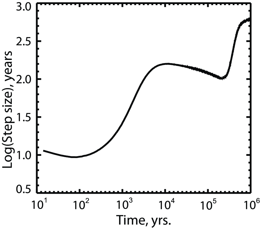
Figure 1: The Monte Carlo time step as a function of time in the model of the chemical evolution of a dense cloud.

where $X_{i}$ is the abundance of species after the $i$th time step, the $\Delta t_{i}$ is the time step in seconds and $N$ is the amount of time steps over which the averaging is performed. In such an averaging procedure, the noise in the random variable $X_{i}$ decreases with $N$ as $\sqrt{N}$ and enables us to resolve abundances below $10^{-12}$. In our simulations we averaged abundances over $10^{6}$ time steps. Therefore, the resolution of our calculations is about 10${}^{-15}-10^{-16}$ cm^-3. The average value of the Monte Carlo time step in Gillespie’s algorithm is equal to an inverse sum of rates of all chemical reactions in the model. For example, in the dense cloud model many molecules form rapidly at initial times and less actively toward the end of evolution (Fig. 1). Time intervals, corresponding to $10^{6}$ time steps in a medium with density $10^{4}$ cm^-3 vary from 10 to $7\cdot 10^{2}$ years for early and late time moments, correspondingly.

4 Comparison of the Monte Carlo method with rate equations

While the Monte Carlo (MC) technique seems to be the most adequate method to solve the chemical master equation, it is computationally extremely demanding. Rate equations (RE) do not account for the stochastic nature of surface processes and thus may produce spurious results in some circumstances. On the other hand, they do require much less computer power and are easier to handle. Therefore rate equations will remain an important tool in theoretical astrochemistry.

Given the importance of surface processes, it is thus necessary to isolate regions in the parameter space where rate equations should not be used at all or, at least, should be used with caution. Similar comparisons, having been made so far, are based on a very limited number of species and reactions (e.g. Charnley, 1998, 2001; Ruffle & Herbst, 2000; Green et al., 2001; Caselli et al., 2002; Stantcheva et al., 2002; Stantcheva & Herbst, 2003, 2004; Lipshtat & Biham, 2003; Barzel & Biham, 2007; Chang et al., 2007). As we implemented a unified Monte Carlo approach to the gas-phase and surface chemistry, which is capable to treat a “regular size” chemical network, we are able to perform a comprehensive comparison between predictions of the MC and the (M)RE approaches.

For both the Model T and the Model H, the rate equations (RE), the modified rate approach (MRE) (for surface chemistry) and the Monte Carlo method are used to simulate gas-phase and surface chemistry. The differences in abundances discussed are related to surface chemistry and/or dust-gas interactions. For the gas-phase chemistry, all models produce identical results. Each run represents a combination of the tunneling treatment (T or H) and the surface chemistry treatment (RE, MRE, or MC). In total, we considered six models denoted as T-RE, T-MRE, etc.

4.1 Global Agreement

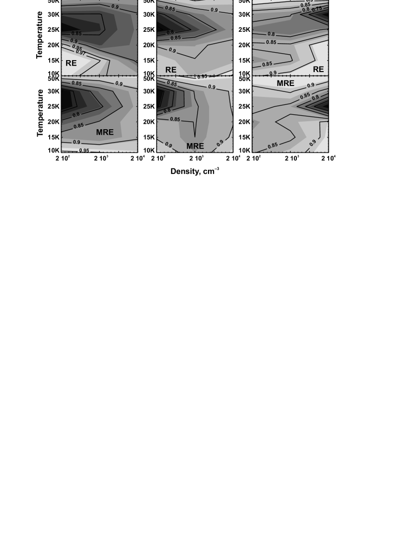
Figure 2: Global agreement diagrams for Model T at three time moments. Percentage of species is shown in contour labels, for which abundances computed with the rate equations and with the Monte Carlo method differ by no more than an order of magnitude. Grayscale map with arbitrary contours is added for clarity. Darker color corresponds to worse agreement. Results are presented for conventional rate equations (top row) and for modified rate equations (bottom row).

To perform an overall comparison, in Figures 2 and 3 we show diagrams of global agreement between MC, RE, and MRE calculations as a function of $n$ and $T$ for evolutionary times $10^{4}$, $10^{5}$, and $10^{6}$ years. For a given species, the two methods, being compared, are assumed to agree at time $t$ if they produce abundances, that differ by no more than an order of magnitude. As we have mentioned above, in the MC method we are able to resolve abundances down to $10^{-15}$, which would lead to a formal disagreement between abundances, say, $10^{-15}$ in the MC method and $10^{-16}$ (or smaller) in the RE method (all abundances are relative to the total number of H atoms). This kind of disagreement is not meaningful from the observational point of view because such small relative abundances are extremely difficult to observe with a satisfactory accuracy. In addition, even though lower abundances can be calculated by the RE method, their actual accuracy is limited by the numerical interpolation. In the following discussion, species, for which both methods predict relative abundances less than $10^{-12}$, are excluded from further consideration. In Figures 2 and  3, contours labeled with 0.9 mean that the two methods give abundances that differ by less than an order of magnitude for 90% of species with abundances higher than $10^{-12}$ in both methods.

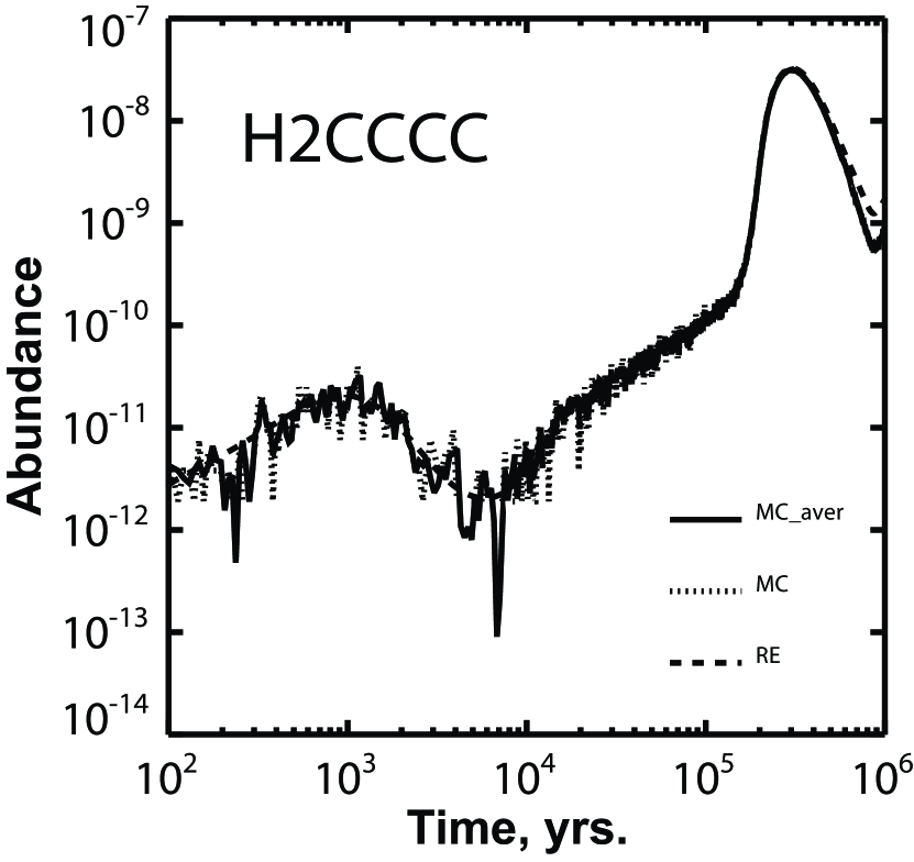
Figure 4: Evolution of H₂CCCC gas-phase abundance at $n=2\cdot 10^{4}$ cm^-3 and $T=10$ K, simulated with the MC and RE methods (Model T). Dotted line indicates raw MC results, solid line shows MC results after averaging. Results of RE integration are shown with dashed line.

An order-of-magnitude agreement criterion may seem to be too coarse. However, when stochastic effects do not play an important role, all three method produce results, which are nearly identical. To illustrate this, we show in Figure 4 the evolution of the H₂CCCC abundance at $n=2\cdot 10^{4}$ cm^-3 and $T=10$ K, simulated with the MC and RE methods. The species is chosen because its abundance strongly varies with time. It can be seen that the difference between the two methods is very small.

4.1.1 Model T

In Model T the species are highly mobile—atomic and molecular hydrogen because of tunneling, and all the other species because of the low energy barrier for diffusion. Mobility drives rapid surface reactions with rates which sometimes exceed the accretion/desorption rate. Surface reactions, which are on average faster than accretion, are not permitted in the MC approach when surface populations of their reagents are low ($\sim$ 1), but they are allowed in the RE approach, where the surface abundance of a species can be much less than one. Because of that, differences between Monte Carlo and rate equation methods are quite noticeable in Model T.

At temperatures below 20 K and above $\sim 40$ K the agreement between the stochastic method and the rate equation method (both RE and MRE) is about 85% or better at all times and densities (Figure 2). Around $T\sim 10$ K the residual discrepancy is mainly caused by complex surface species, which have zero abundances in Model T-MC and are overproduced in Model T-RE and Model T-MRE, so that their abundances are just above the adopted cutoff of $10^{-12}$. If we would raise the cutoff to $10^{-11}$, the agreement would be almost 100%. At $T\sim 50$ K the agreement is also nearly perfect, as the chemistry is almost a purely gas-phase chemistry under these conditions (dust temperature being equal to gas temperature).

All the major discrepancies are concentrated in the temperature range between 25–30 K. In this range the accretion rate (which depends on gas temperature) is high enough to allow accumulation and some processing of surface species, while the correspondingly high desorption rate (which depends on dust temperature and $A_{\rm V}$) precludes surface production of complex molecules. The latter process is adequately described in the MC runs only.

At earlier times ($t\lesssim 10^{5}$ years) the largest differences in this temperature range are observed at lower densities. They are caused by an overproduction of ‘terminal’ surface species, like water, ammonia, hydrogen peroxide, carbon dioxide, etc., in the RE and MRE calculations. At later times ($t\sim 10^{6}$ years) situation changes drastically. The discrepancies shift toward higher density, and the overall agreement falls off to about 60% for both RE and MRE calculations. Even though the stochastic chemistry is only important on dust surfaces, by this time it also influences many gas-phase abundances due to effective gas-grain interactions.

At $t=10^{6}$ years, in the RE calculation at $T=30$ K, among 234 species with abundances higher than $10^{-12}$, 95 species (including 81 gas-phase species) have an order of magnitude disagreement with the MC run. In the MRE run at $T=25$ K, the number of species with abundances above $10^{-12}$ is 221. Among them 83 species disagree with the MC results by more than an order of magnitude. In both calculations these are mostly carbon-bearing species, like CO, CO₂, CS, to name a few, and, in particular, carbon chains (like some cyanopolyynes). It is noteworthy that not only the abundances of neutral species disagree, but also the abundances of some ions, including C⁺ and S⁺.

4.1.2 Model H

In Model H the mobility of all species on the surface (including H and H₂) is caused by thermal hopping only, which is slow because of the high $E_{\rm b}/E_{\rm D}$ ratio. One of the consequences of these slow surface reaction rates is that results produced by the modified rate equations almost do not differ from results of conventional rate equations. The essence of the modification is to artificially slow down surface reactions to make their rates consistent with accretion/desorption rates. In Model H all surface reactions are slow anyway, so that modifications never occur. Thus, we only compare the results of the MC and RE calculations.

At $t=10^{4}$ years the percentage agreement between the two runs never falls below 80% and most often is actually much better than the adopted order-of-magnitude criterion. At later times, the discrepancy appears in the same temperature range as in Model T, i.e., between 25 and 30 K. Unlike Model T, both at $t=10^{5}$ years and $t=10^{6}$ years the disagreement shows up at low density. The set of discrepant species is nearly identical at both times and consist mostly of ices, overproduced by rate equations. These ices include some key observed species. For example, NH₃, H₂O, CO₂ ices are all abundant in the Model H-RE despite the low density, with a surface H₂O abundance reaching $3\cdot 10^{-7}$ by $10^{6}$ years. On the other hand, the Model H-MC results in very small or zero abundances for the same species. More chemically rich ices in Model H-RE bring about enhanced gas-phase abundances for the same molecules. The only species which is underproduced by the rate equation approach is surface C₂O.

4.2 Selected Species

The diagrams presented above indicate areas in the parameter space, relevant to molecular clouds, where deterministic methods fail to describe stochastic surface processes. However, a global agreement does not necessarily imply that the abundances of key species are also correctly calculated. In the following we discuss a few important gas-phase species and ices, for which an order of magnitude (or more) disagreement has been found.

4.2.1 Model T

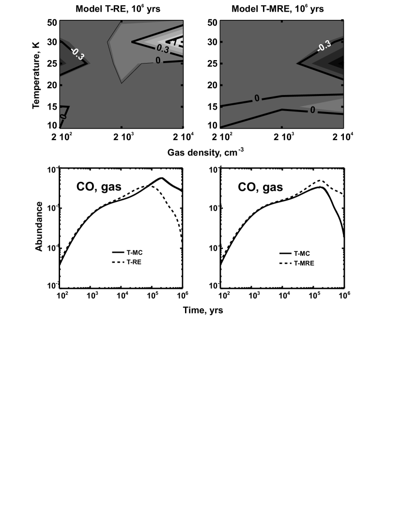
Figure 5: (Top row) Agreement diagrams for CO in Model T. Contour labels correspond to the logarithm of the ratio of gas-phase CO abundance in the MC run to that in the RE (top left) and MRE (top right) runs. (Bottom row) Gas-phase CO abundance evolution in the RE run ($n=2\cdot 10^{4}$ cm^-3 and $T=30$ K; bottom left) and in the MRE run ($n=2\cdot 10^{4}$ cm^-3 and $T=25$ K; bottom right).

Because surface reaction rates are high in this model, there are many species for which stochastic and deterministic methods give quite different results. The most abundant trace molecule, CO, is among these species. In Figure 5, we show agreement diagrams for Models T-RE and T-MRE (top row) and the CO abundance evolution for $n-T$ combinations corresponding to the worst agreement. Both the RE and MRE methods fail to reproduce the late CO evolution at high density and temperatures of 25–30 K (where the global agreement is also worst in this model), but each in a different way. While in Model T-RE CO is underabundant by an order of magnitude, in Model T-MRE it is overabundant by the similar amount. This difference is related to the treatment of CO $\longrightarrow$ CO₂ conversion on dust surfaces, where underabundance of the CO ice in Model T-RE and overabundance in Model T-MRE are observed at almost all times. At later time, these surface abundances just start to propagate to gas-phase abundances.

Overproduction of the CO₂ ice in Model T-RE also consumes carbon atoms which would otherwise be available not only for CO, but also for more complex molecules, in particular, carbon chains, starting from C₂, observed in diffuse clouds, and C₂S, used as a diagnostics in prestellar cores. In the RE and MRE calculations these molecules, like CO, show trends opposite to that of CO₂ ice: when surface CO₂ is overabundant with respect to the MC model, carbon chains are underabundant and vice versa.

When CO molecule sticks to a grain, it either desorbs back to the gas-phase, where it may participate in further processing, or is converted into CO₂. As the desorption energy is quite high for CO₂, it acts as a sink for carbon atoms at these temperatures. In the accretion-limited regime, rate equations overproduce CO₂ with respect to the MC method. Thus, we see less CO and other carbon-bearing species in the gas-phase. The MRE method helps, probably, too much to account for accretion-limited CO processing and essentially quenches surface CO $\longrightarrow$ CO₂ conversion. It is worth noting that at high density in this particular temperature range (and for adopted CO desorption energy) CO balances between complete freeze-out (at $T<20$ K) and near absence on dust surface (at $T>30$ K). Thus, even relatively minor changes in treatment may lead to noticeable consequences.

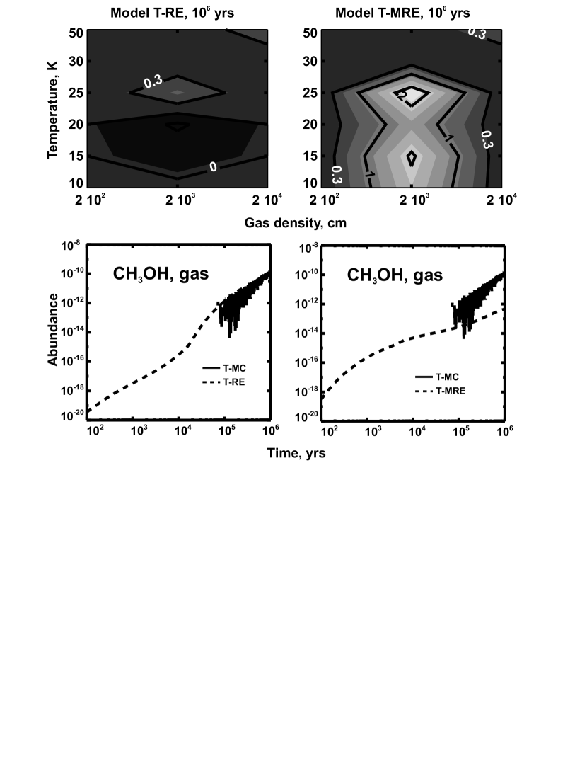
Figure 6: (Top row) Agreement diagrams for methanol. Contour labels correspond to the logarithm of the ratio of gas-phase CH₃OH abundance in the MC run to that in the RE (top left) and MRE (top right) runs. (Bottom row) Gas-phase methanol abundance evolution in the RE run ($n=2\cdot 10^{3}$ cm^-3 and $T=25$ K; bottom left) and in the MRE run ($n=2\cdot 10^{3}$ cm^-3 and $T=25$ K; bottom right).

Another carbon-bearing molecule that shows an interesting behavior is methanol in the gas phase. Diagrams, comparing its abundance computed with the MC approach and with the rate equations, are presented in Figure 6. The agreement between results of the MC calculations and the RE calculations is almost perfect, at least, within the scatter produced by the MC simulations. However, the modified rate equations, which tend to improve agreement between stochastic and deterministic methods for many other species, in this particular case underpredict methanol abundance by more than two orders of magnitude in comparison with the MC run. The same is true for surface methanol as well. It is interesting to note that the region in the parameter space, where MC and MRE methanol abundances disagree, extends down to lowest temperatures considered.

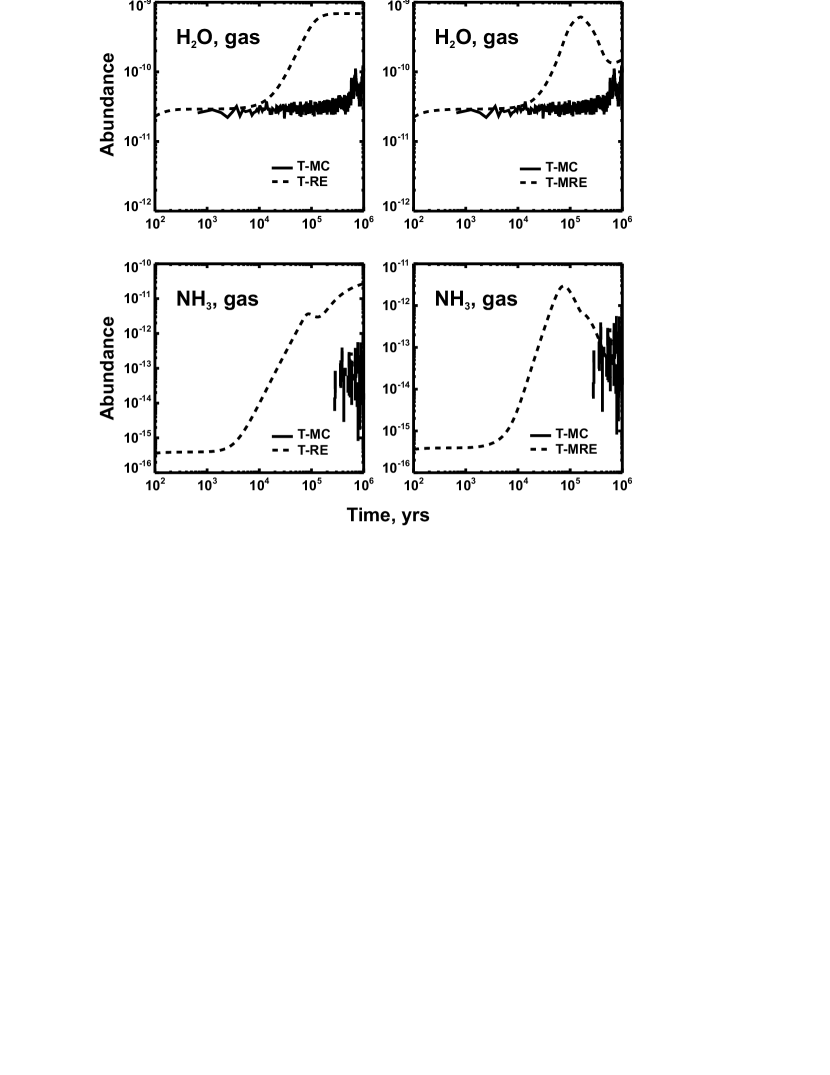
Figure 7: Water and ammonia gas-phase abundance evolution in the RE run in Model T ($n=2\cdot 10^{2}$ cm^-3 and $T=25$ K; left) and in the MRE run ($n=2\cdot 10^{2}$ cm^-3 and $T=25$ K; right).

An interesting pattern is presented by the abundance of water, ammonia and their ices (Figure 7). These species are severely overproduced by the RE methods at $t=10^{5}$ years, but after this time the modified rate equations are able to restore the agreement with the MC method, so that by $10^{6}$ years difference between MC and MRE runs is not significant. This is an example of a situation where the MRE help to produce realistic results, at least, at later times. We show plots only for gas-phase abundances because these are what is really observed. However, these abundances are only a reflection of surface processes, and surface water and ammonia abundances behave in exactly the same way. It is hard to name a single reaction which is responsible for the difference between results of RE and MRE methods in this case. Let’s consider water as its chemistry is somewhat simpler. The primary formation reaction for water is H + OH, with only a minor contribution from H₂O₂ (see below). However, hydroxyl is not produced in H + O reaction, as one might have expected. Because of the paucity of H atoms on the grain surface, hydroxyl formation is dominated by reaction

$${\rm O}+{\rm HNO}\longrightarrow{\rm NO}+{\rm OH}.$$

Abundance of HNO is restored in reaction

$${\rm H}+{\rm NO}\longrightarrow{\rm HNO}.$$

These two reactions form a semi-closed loop for which the sole result is OH synthesis out of an H atom and an O atom. Evolution of surface O abundance seems to be the key to the difference between the RE and MRE models. In the RE model the number of O atoms on a surface is determined by the balance between their accretion from the gas phase and consumption in O + HNO reaction. The same processes define O abundance in the MRE model as well, but only at $t\lesssim 10^{5}$ years. After this time O+HNO reaction slows down significantly due to modifying correction, and O abundance is controlled purely by accretion and desorption thereafter (as it is in the MC model at all times). As a result, OH and H₂O abundances decrease, getting closer to the MC model prediction. A similar mechanism is at work in the case of ammonia as well.

4.2.2 Model H

The only parameter region where a discrepancy occurs for Model H is located at $n=2\cdot 10^{2}$ cm^-3 and $T=25$ K. Because of the low density, the degree of molecular complexity at these conditions is also low, and by $10^{6}$ years only 73 species have abundances higher than $10^{-12}$ at least in one of the calculations. Of these 73 species, 25 show disagreement between the MC calculations and the RE calculations.

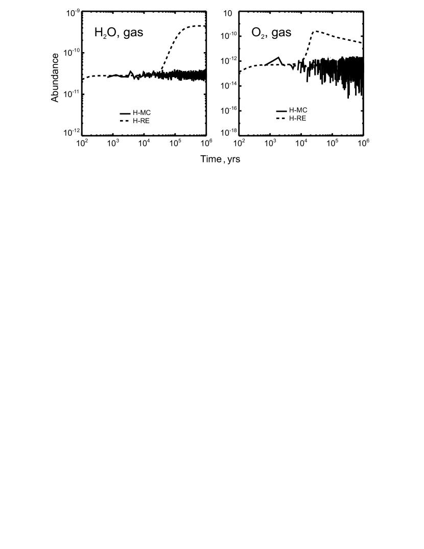
Figure 8: Water and molecular oxygen abundances at $n=2\cdot 10^{2}$ cm^-3 and $T=25$ K in Model H.

In the top row of Figure 8 we show the low density evolution of gas-phase water and molecular oxygen abundances. Both plots show a similar trend. In the MC calculations the abundance of the molecule stays nearly constant. At earlier times this steady-state behavior is reproduced in the RE run as well, but later the abundance grows and exceeds the MC abundance by more than an order of magnitude. It is interesting to note that the average O₂ abundance in the MC run seems to decrease somewhat at later times, and this trend is reproduced by the RE model. The behavior of gas-phase abundances is a reflection of grain-surface abundances. It must be kept in mind that surface water abundance is quite high in the H-RE model, reaching almost $10^{-6}$. Even though evaporation rate is not very high, it does increase gas-phase abundance up to a level of a few time $10^{-10}$. Also, it is a low density model, so desorption is primarily caused by photons.

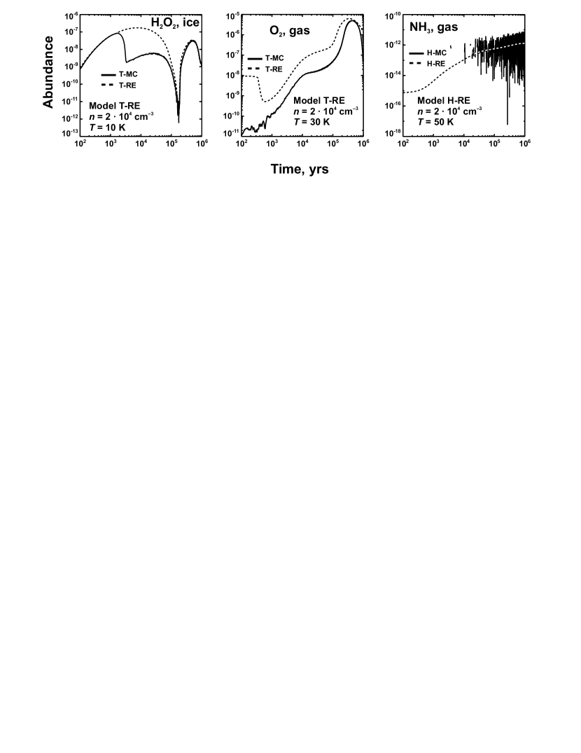
Figure 9: Abundance evolution for selected species. Models and physical conditions are indicated on the diagrams.

In Figure 9 we show the evolution of H₂O₂ surface abundance and O₂ gas-phase abundance in Model T-RE at $n=2\cdot 10^{4}$ cm^-3 and the gas-phase ammonia abundance in Model H-RE at $n=2\cdot 10^{3}$ cm^-3. These plots demonstrate that disagreement does not always mean simply higher or lower abundances. Different processes determine the H₂O₂ abundance at different times, and while the RE method is able to capture some of these processes, others are obviously missed. Our analysis shows that this behavior is related to the treatment of reaction with H atoms. Specifically, surface abundance of H₂O₂ is controlled by three reactions only. It is produced in a reaction H + O₂H and destroyed by atomic hydrogen in reactions producing either H₂O + OH or O$+2$H + H₂. (Note that in the considered model water ice is almost irreversible sink for O atoms as there are no surface reactions destroying water, and desorption is negligible.) The formation reaction is fast as it does not have an activation barrier. So, initially, as H and O atoms start to stick to a grain, surface abundance of H₂O₂ steadily grows. At the same time, there is not enough H atoms for either of destruction reactions. Then, in the MC model at around 1300 years the first destruction reaction (H + H₂O₂ $\longrightarrow$ H₂O + OH), which has a slightly lower activation barrier than the other one (H + H₂O₂ $\longrightarrow$ O₂H + H₂), starts to “steal” some hydrogen atoms from the formation reaction, irreversibly removing one O atom per reaction from the H₂O₂ (re)formation process. This is the reason for the sharp fall-off of H₂O₂ abundance. On the other hand, in the RE model both destruction and formation reactions may occur simultaneously, which prevents the first destruction reaction from having such a dramatic effect. Note that the second reaction restores an O₂H molecule which may react again with an H atom to restore an H₂O₂ molecule.

H₂O₂ is not unique in this kind of behavior. There are some other surface species which show more or less similar trends, that is, almost perfect agreement at some times and quite noticeable disagreement at other times. These are some carbon chains (C₂H₂, C₂N) or simpler molecules (CS, NO). Another equally dramatic example is represented by C₂H₂. The mechanism is similar, that is, it is related to the sequence of hydrogen additions which is treated differently in the MC model and the RE model.

Evolution of the O₂ abundance computed with the RE method follows the evolution computed with the MC model, but most of the time the RE curve is somewhat higher than the MC curve. Finally, the plot for ammonia shows the situation when the RE method correctly describes the average abundance evolution. However, the abundance predicted by the MC method fluctuates so wildly, that at each particular $t$ we can detect disagreement with high probability, using our formal order-of-magnitude criterion.

5 Discussion

In the previous sections we investigated the validity of the (modified) rate equation approach to grain surface chemistry under different physical conditions encompassing diffuse clouds, giant molecular clouds, infrared dark clouds etc. Evolution of the medium is studied with an extended gas-grain chemical model over a time period of 10⁶ years. We utilize the unified stochastic Monte Carlo approach, applied simultaneously to gas-phase and grain-surface reactions. The results are used to test the validity of conventional deterministic approaches. In general, differences in results obtained with deterministic and stochastic methods strongly depend on the adopted microphysical model of surface chemistry. In Model T, where tunneling for atomic and molecular hydrogen is permitted and diffusion/desorption energies ratio is low ($E_{\rm b}/E_{\rm D}=0.3$), discrepancy both for RE and MRE methods is very significant. At low temperatures (10 - 20 K) only abundances of surface species are discrepant by more than an order of magnitude. At moderate temperatures (25–40 K), due to active gas-grain interaction, incorrect treatment of grain surface chemistry becomes important for gas-phase abundances, too, and leads to dramatic decrease of overall agreement. At even higher temperatures agreement becomes better again due to limited surface chemistry. In Model H with no tunneling and high $E_{\rm b}/E_{\rm D}$ ratio, surface species are much less mobile, and the agreement between deterministic and stochastic methods is better. The only exception is low density ($n({\rm H})=10^{2}$ cm^-3) with moderate temperatures (25 – 30 K), where average residence time of species on grain surface is still lower than the average interval between reaction events. In general, the stochastic chemistry severely affects abundances and, thus, must be taken into account in chemical models of a warm and moderately dense medium.

Modifications in rate equations, aimed at taking into account the accretion-limited regime, do not provide a significant improvement over ‘canonical’ rate equations in Model T. Close inspection of Figure 2 shows that at earlier times ($t\leq 10^{5}$ years) modified rate equations mostly produce results, which are rather less consistent with the ‘exact’ Monte Carlo solution, than results of the RE method. Only at later times ($t\sim 10^{6}$ years) results of the MRE method become more consistent with the ‘exact’ solution than the RE results. In the previous section, we have already shown some examples of species, for which the MRE method actually worsens the agreement.

Because at many of considered physical conditions results obtained with Monte Carlo method deviate significantly from those obtained with (modified) rate equations, the natural question to ask is whether the inability of the RE method to treat these combinations of parameters might have caused mis-interpretation of observational data. To answer this question, one would need to consider an object, for which a large volume of observational data is available, so that simultaneous comparison for many molecules is possible. So far, there seems to be just one molecular cloud, which is studied in necessary details. This is a sub-region of the TMC1 cloud where cyanopolyynes reach high concentrations, the so-called TMC1-CP. The physical conditions in this object ($T\sim 10$ K, $n_{\rm H}\sim 10^{4}$ cm^-3) do fall into the range adopted in our model (Benson & Myers, 1989). However, the TMC1-CP is probably too cold to show significant dependence of gas-phase abundances from surface processes.

We may expect that the disagreement will be more significant in hotter objects. The range of physical conditions studied in this paper is quite narrow, as it has only been chosen to provide an initial view on the importance of stochastic treatment for surface chemistry. There are two directions which are worth to follow for further study. One of them is related to diffuse clouds. In this paper we most of the time assumed initial conditions in which all the hydrogen is molecular even at low density. Another simplification, which is, strictly speaking, not valid in low density medium, is equality of dust and gas temperature. So, it is interesting to check if stochastic effects work in predominantly atomic gas with different gas and dust temperatures. Another direction is chemistry at later stages of star formation, that is, in hot cores, hyper- and ultracompact HII regions, protoplanetary disks. In particular, in dark cold disk midplanes, which are poor in atomic hydrogen, stochastic effects may severely influence surface synthesis of hydrogenated species, like formaldehyde, which are later transferred by turbulent mixing in warmer disk areas and desorbed into gas phase (Aikawa, 2007). In these circumstances one would definitely need to use more accurate methods to model surface chemistry. Stochastic effects may be even more pronounced in the dynamically evolving medium, like during slow warm-up phase in hot cores or “corinos”. Complex (organic) molecules will be among the most affected species.

While the Monte Carlo method is the most direct approach, it is by no means practical. So, other methods are to be developed, in particular, the method of moment equations, if we want to understand deeper the chemical evolution in warm and dense astrophysical objects.

6 Conclusions

In this study, a gas-grain chemical model is presented, consisting of about 600 species and 6000 reactions with stochastic description of grain surface chemistry. For the first time both gas phase and grain surface reactions are simulated with a unified Monte Carlo approach. This unified model is used to test the validity of rate equations and modified rate equations for a set of physical conditions, relevant to translucent clouds, dark dense cores, and infrared dark clouds.

A comparison of results obtained with deterministic rate equations (RE) and modified rate equations (MRE) with results of Monte Carlo simulations was performed for this set of physical conditions and two different models of surface chemistry. We found that results obtained with both RE and MRE approaches sometimes significantly deviate from those obtained with Monte Carlo calculations in Model T, where surface species are highly mobile and most of the grain chemistry occurs in the accretion limited regime. While at low temperatures (10 K – 20 K) mainly RE and MRE abundances of surface species show significant discrepancies, at moderately high temperatures (25 K – 30 K) even abundant gas-phase species like CO considerably deviate from the Monte Carlo results. At these temperatures grain surface chemistry is still very active and at the same time processes of accretion and desorption are very efficient. The gas-phase abundances of many species are influenced by surface chemistry that is correctly described in Monte Carlo simulations only. In Model H surface species are much less mobile than in Model T and the agreement between the (modified) rate equations approach and Monte Carlo simulations is almost perfect. The only parameter region where this discrepancy is significant is at a temperature of $T=25$ K and at a low density $n({\rm H})=2\cdot 10^{2}$ cm^-3. On the whole, results of modified rate equations seem to be in somewhat closer agreement with Monte Carlo simulations than results of the conventional rate approach. But still, the agreement is far from being perfect, so modified rates should be used with care. We conclude that stochastic effects have a significant impact on chemical evolution of moderately warm medium and must be properly taken into account in corresponding theoretical models. In the studied parameter range, stochastic effects are, in general, not important at low ($T\sim 10$ K) and high ($T\sim 50$ K) temperatures.

Table 1: Adopted surface chemistry models

Model	Based on	Tunneling	$E_{\rm b}/E_{\rm D}$
T	Hasegawa et al. (1992)	Yes	0.3
H	Katz et al. (1999)	No	0.77

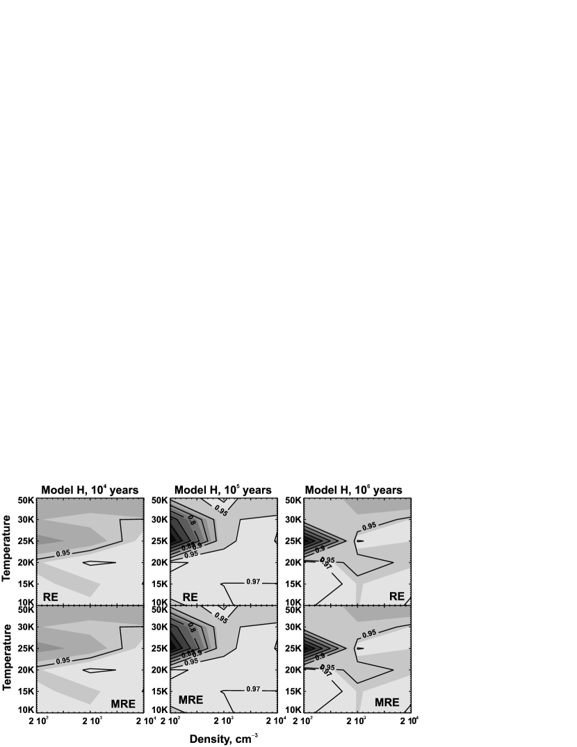
Figure 3: Same as in Figure 2, but for Model H.

References

- Aikawa (2007) Aikawa, Y. 2007, ApJ, 656, L93
- Barzel & Biham (2007) Barzel, B. & Biham, O. 2007, ApJ, 658, L37
- Benson & Myers (1989) Benson, P. J. & Myers, P. C. 1989, ApJS, 71, 89
- Biham et al. (2001) Biham, O., Furman, I., Pirronello, V., & Vidali, G. 2001, ApJ, 553, 595
- Boger & Sternberg (2006) Boger, G. I. & Sternberg, A. 2006, ApJ, 645, 314
- Caselli et al. (1998) Caselli, P., Hasegawa, T. I., & Herbst, E. 1998, ApJ, 495, 309
- Caselli et al. (2002) Caselli, P., Stantcheva, T., Shalabiea, O., Shematovich, V. I., & Herbst, E. 2002, Planet. Space Sci., 50, 1257
- Cazaux & Tielens (2004) Cazaux, S. & Tielens, A. G. G. M. 2004, ApJ, 604, 222
- Chang et al. (2005) Chang, Q., Cuppen, H. M., & Herbst, E. 2005, A&A, 434, 599
- Chang et al. (2007) —. 2007, A&A, 469, 973
- Charnley (1998) Charnley, S. B. 1998, ApJ, 509, L121
- Charnley (2001) —. 2001, ApJ, 562, L99
- Cuppen & Herbst (2007) Cuppen, H. M. & Herbst, E. 2007, ApJ, 668, 294
- Draine & Lee (1984) Draine, B. T. & Lee, H. M. 1984, ApJ, 285, 89
- Garrod & Herbst (2006) Garrod, R. T. & Herbst, E. 2006, A&A, 457, 927
- Gillespie (1976) Gillespie, D. T. 1976, Journal of Computational Physics, 22, 403
- Green et al. (2001) Green, N. J. B., Toniazzo, T., Pilling, M. J., Ruffle, D. P., Bell, N., & Hartquist, T. W. 2001, A&A, 375, 1111
- Hasegawa et al. (1992) Hasegawa, T. I., Herbst, E., & Leung, C. M. 1992, ApJS, 82, 167
- Hassel et al. (2008) Hassel, G. E., Herbst, E., & Garrod, R. T. 2008, ApJ, 681, 1385
- Herbst & Shematovich (2003) Herbst, E. & Shematovich, V. I. 2003, Ap&SS, 285, 725
- Katz et al. (1999) Katz, N., Furman, I., Biham, O., Pirronello, V., & Vidali, G. 1999, ApJ, 522, 305
- Le Bourlot et al. (1993) Le Bourlot, J., Pineau des Forets, G., Roueff, E., & Schilke, P. 1993, ApJ, 416, L87+
- Lee et al. (1996) Lee, H.-H., Herbst, E., Pineau des Forets, G., Roueff, E., & Le Bourlot, J. 1996, A&A, 311, 690
- Lee et al. (1998) Lee, H.-H., Roueff, E., Pineau des Forets, G., Shalabiea, O. M., Terzieva, R., & Herbst, E. 1998, A&A, 334, 1047
- Lipshtat & Biham (2003) Lipshtat, A. & Biham, O. 2003, A&A, 400, 585
- Lipshtat et al. (2004) Lipshtat, A., Biham, O., & Herbst, E. 2004, MNRAS, 348, 1055
- Perets et al. (2005) Perets, H. B., Biham, O., Manicó, G., Pirronello, V., Roser, J., Swords, S., & Vidali, G. 2005, ApJ, 627, 850
- Pirronello et al. (1997a) Pirronello, V., Biham, O., Liu, C., Shen, L., & Vidali, G. 1997a, ApJ, 483, L131+
- Pirronello et al. (1999) Pirronello, V., Liu, C., Roser, J. E., & Vidali, G. 1999, A&A, 344, 681
- Pirronello et al. (1997b) Pirronello, V., Liu, C., Shen, L., & Vidali, G. 1997b, ApJ, 475, L69+
- Roberts et al. (2004) Roberts, H., Herbst, E., & Millar, T. J. 2004, A&A, 424, 905
- Ruffle & Herbst (2000) Ruffle, D. P. & Herbst, E. 2000, MNRAS, 319, 837
- Semenov et al. (2003) Semenov, D., Henning, T., Helling, C., Ilgner, M., & Sedlmayr, E. 2003, A&A, 410, 611
- Semenov et al. (2004) Semenov, D., Wiebe, D., & Henning, T. 2004, A&A, 417, 93
- Shalabiea & Greenberg (1995) Shalabiea, O. M. & Greenberg, J. M. 1995, A&A, 296, 779
- Snow & McCall (2006) Snow, T. P. & McCall, B. J. 2006, ARA&A, 44, 367
- Spitzer & Tomasko (1968) Spitzer, L. J. & Tomasko, M. G. 1968, ApJ, 152, 971
- Stantcheva et al. (2001) Stantcheva, T., Caselli, P., & Herbst, E. 2001, A&A, 375, 673
- Stantcheva & Herbst (2003) Stantcheva, T. & Herbst, E. 2003, MNRAS, 340, 983
- Stantcheva & Herbst (2004) —. 2004, A&A, 423, 241
- Stantcheva et al. (2002) Stantcheva, T., Shematovich, V. I., & Herbst, E. 2002, A&A, 391, 1069
- Tielens & Hagen (1982) Tielens, A. G. G. M. & Hagen, W. 1982, A&A, 114, 245
- van Dishoeck et al. (2006) van Dishoeck, E. F., Jonkheid, B., & van Hemert, M. C. 2006, in Faraday Discussions 133: Chemical Evolution of the Universe, ed. I. R. Sims & D. A. Williams, 231–243
- van Zadelhoff et al. (2003) van Zadelhoff, G.-J., Aikawa, Y., Hogerheijde, M. R., & van Dishoeck, E. F. 2003, A&A, 397, 789
- Vasyunin et al. (2008) Vasyunin, A. I., Semenov, D., Henning, T., Wakelam, V., Herbst, E., & Sobolev, A. M. 2008, ApJ, 672, 629
- Woodall et al. (2007) Woodall, J., Agúndez, M., Markwick-Kemper, A. J., & Millar, T. J. 2007, A&A, 466, 1197