Thermodynamics of SU(3) gauge theory at fixed lattice spacing
Abstract:
We study thermodynamics of SU(3) gauge theory at fixed scales on the lattice, where we vary temperature by changing the temporal lattice size . In the fixed scale approach, finite temperature simulations are performed on common lattice spacings and spatial volumes. Consequently, we can isolate thermal effects in observables from other uncertainties, such as lattice artifact, renormalization factor, and spatial volume effect. Furthermore, in the EOS calculations, the fixed scale approach is able to reduce computational costs for zero temperature subtraction and parameter search to find lines of constant physics, which are demanding in full QCD simulations. As a test of the approach, we study the thermodynamics of the SU(3) gauge theory on isotropic and anisotropic lattices. In addition to the equation of state, we calculate the critical temperature and the static quark free energy at a fixed scale.
1 Introduction
Since finite temperature () lattice QCD is performed on lattice with a temporal extent , qualitative calculations at high may require lower simulation cost than that at . However quantitative systematic studies at need huge simulation cost often more than that at . Because such study requires calculations at wide range of lattice scale. It is a reason why recent large scale thermodynamics calculations are often performed with the Staggered type quark formulations [1], which needs lower computational cost than that with Wilson type formulations [3], the domain wall and overlap quarks are all the more costly. To make matters worse, some Wilson type quarks sometimes cause some problems at coarse lattice, e.g. nonperturbative clover coefficient is reliably determined at fm or finer [4], and the domain wall quarks encounter with strong residual quark mass effects at coarse lattice [5]. In spite of the difficulties, results at with the Wilson type quark formulations are desired, because the Staggered type quarks suffer from problems of the flavor symmetry violation and the rooted Dirac operators.
Therefore we propose an alternative fixed scale approach to study thermodynamics of QCD, where we vary by varying the temporal lattice size instead of the conventional fixed approach. In the fixed scale approach, results are common for each () simulations. It may be able to reduce total simulation cost drastically. Furthermore, common parameters (except for ) enable us to investigate pure thermal effects of observables without obstacles coming from changing lattice spacing and spatial volume effects.
In this report, we test the approach in the SU(3) gauge theory on isotropic and anisotropic lattices. Our lattice action and some details of the EOS calculation are given in Sect.2.1 and Sect.2.2. Results of EOS are presented in Sects.2.3 and 2.4. The and the static quark free energy are discussed in Sect.3 and 4. We conclude in the last section.
2 Equation of state
2.1 T-integration method
In the fixed scale approach, to calculate the pressure non-perturbatively, we propose a new method, “the T-integral method” [6] :
| (1) |
based on another thermodynamic relation valid at vanishing chemical potential:
| (2) |
The initial temperature is chosen such that . Calculation of requires the beta functions just at the simulation point, but no further Karsch coefficients are necessary. Since is restricted to have discrete values, we need to make an interpolation of with respect to .
Since the coupling parameters are common to all temperatures, our fixed scale approach with the -integral method has several advantages over the conventional approach; (i) subtractions can be done by a common simulation, (ii) the condition to follow the LCP is obviously satisfied, and (iii) the lattice scale as well as beta functions are required only at the simulation point. As a result of these, the computational cost needed for simulations is reduced drastically.
When we adopt coupling parameters from spectrum studies, the values of around and below the critical temperature are much larger than those used in conventional fixed studies. For example, at fm, MeV is achieved by . Therefore, for thermodynamic quantities around and below , we can largely reduce the lattice artifacts over the conventional approach, with much smaller total computational cost. This is also a good news for phenomenological applications of the EOS, since the temperature achieved in the relativistic heavy ion collision at RHIC and LHC will be at most up to a few times the [7]. We note here that, as increases, becomes small and hence the lattice artifact increases. Therefore, our approach is not suitable for studying how the EOS approaches the Stephan-Boltzmann value in the high limit.
2.2 Lattice action
We study the SU(3) gauge theory with the standard plaquette gauge action on an anisotropic lattice with the spatial (temporal) lattice size and scale () and (), respectively. The lattice action is given by
| (3) | |||||
| (4) |
where is the plaquette in the plane and and are the bare lattice gauge coupling and bare anisotropy parameters. The trace anomaly is calculated by
| (5) | |||||
| (6) |
with the renormalized anisotropy. is the beta function. vanishes on isotropic lattices.
2.3 EOS on isotropic lattice
Our simulation parameters are listed in Table 1. On isotropic lattices, we calculate EOS on three lattices to study the volume and lattice spacing dependences. The ranges of correspond to –700 MeV for the sets i1 and i2, and –730 MeV for i3, to be compared with MeV. The set a2 will be discussed later. The subtraction is performed with for i1 and i2, and with for i3. We generate up to a few millions configurations using the pseudo-heat-bath algorithm. Statistical errors are estimated by the Jackknife analysis. appropriate bin sizes, which strongly depend on . Typically, bin size of a few thousands configurations are necessary near , while a few hundreds are sufficient off the transition region.
| set | [fm] | [fm] | ||||||
|---|---|---|---|---|---|---|---|---|
| i1 | 6.0 | 1 | 16 | 3-10 | 5.35() | 0.093 | 1.5 | -0.098172 |
| i2 | 6.0 | 1 | 24 | 3-10 | 5.35() | 0.093 | 2.2 | -0.098172 |
| i3 | 6.2 | 1 | 22 | 4-13 | 7.37(3) | 0.068 | 1.5 | -0.112127 |
| a2 | 6.1 | 4 | 20 | 8-34 | 5.140(32) | 0.097 | 1.9 | -0.10704 |
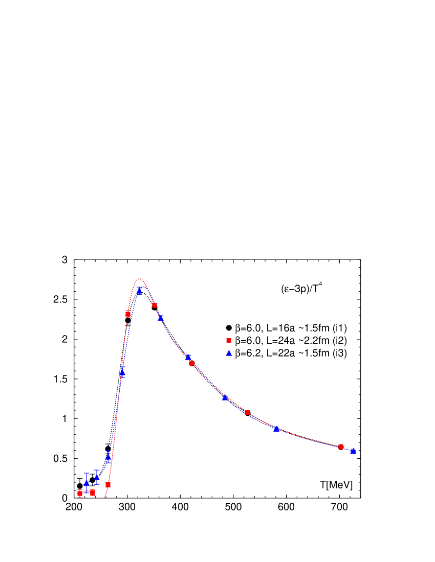
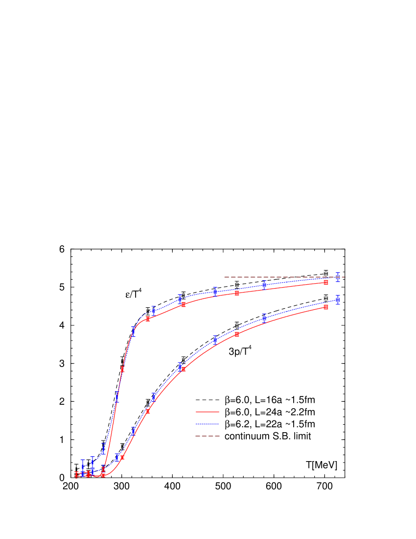
Figure 1 (Left) shows . Dotted lines in the figure are the natural cubic spline interpolations. At and below , lattice size dependence is visible between the sets i1 ( fm) and i2 (2.2 fm). On the other hand, the lattice spacing dependence is small between i1 ( fm) and i3 (0.068 fm). At higher , on three lattices show good agreement. The integration of (1) is performed numerically using the natural spline interpolations shown in Fig.1 (Left). For the initial temperature of the integration, we linearly extrapolate the data at a few lowest ’s because the values of at our lowest are not exactly zero. In this study, we commonly take MeV as the initial temperature which satisfies , and estimate the integration from to the lowest by the area of the triangle. Statistical errors for the results of integration are estimated by a Jackknife analysis [11]. Note that the error in the lattice scale do not affect the dimension less quantity .
In Fig.1 (Right), we summarize the results of EOS on isotropic lattices. is calculated combining the results of and . Since the lattice parameter dependence of is small except for the vicinity of , we find that EOS has a similar shape except for the vicinity of . Near and below , we observe a sizable finite volume effect between fm and fm, while the lattice spacing effects are not so. At large , we note a slight tendency that and decrease as the lattice size becomes larger and the lattice spacing becomes smaller. Our results are qualitatively consistent with the previous results by the conventional fixed method [9], but with much reduced lattice artifacts around due to much larger there.
2.4 EOS on anisotropic lattice
The anisotropic lattice with the temporal lattice finer than the spatial one is expected to improve the resolution of without much increasing the computational cost. To further test the systematic error due to the resolution of , we perform the study with the -integral method on an anisotropic lattice with the renormalized anisotropy . The simulation parameters are given as the set a2 in Table 1, which are the same as those adopted in [10]. We vary –8 corresponding to –1010 MeV. The subtraction is performed with . We generate up to a few millions configurations. The beta function with has calculated in our paper [6], and its value at our simulation point is given in Table 1. For we adopt the result of [12].
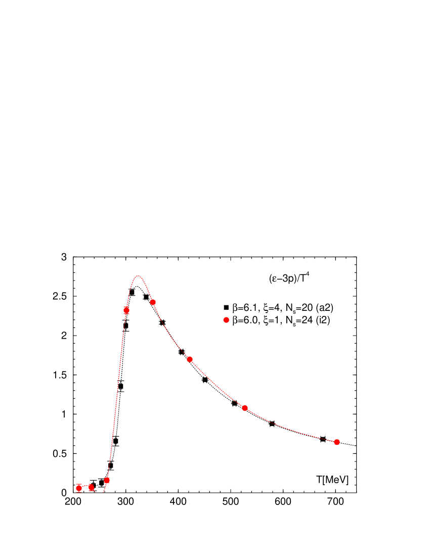
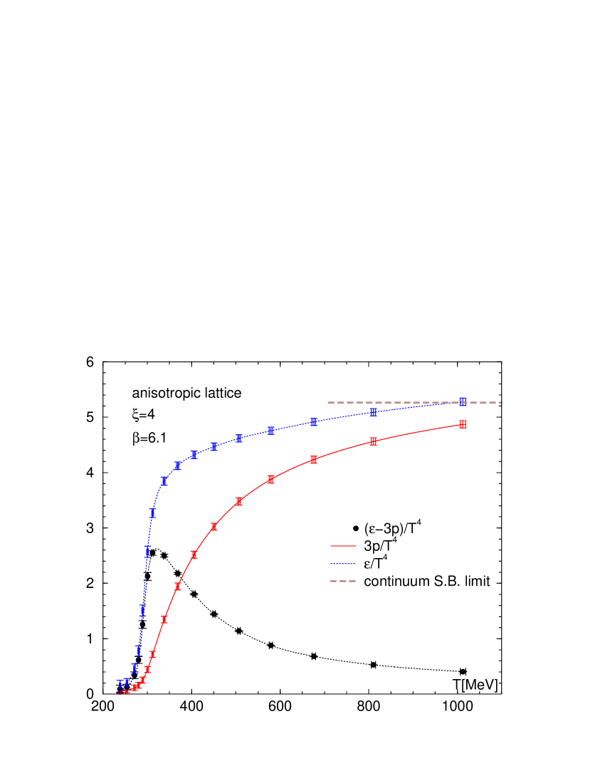
In Fig. 2 (Left), we compare the trace anomaly obtained on the anisotropic lattice with that on the isotropic lattice with similar and (the set i2). We find that the results are generally consistent with each other except for around . We note a systematic tendency that the trace anomaly on the anisotropic lattice is slightly lower than that on the isotropic lattice. According to this tendency, the pressure on the anisotropic lattice is slightly smaller than that on the isotropic lattice at high . The tendency may be understood by the smaller lattice artifact due to the temporal lattice spacing on anisotropic lattices, since lattice artifacts due to temporal lattice spacing are larger than that by the spatial lattice spacings in thermodynamic quantities [13]. Finally, we summarize our results of EOS on the anisotropic lattice in Fig. 2 (Right). We find that they are consistent with those on isotropic lattices.
3 Transition temperature
Here we consider a possibility to compute the in the fixed scale approach. is determined by studying temperature dependence of order parameters. Strictly speaking, such temperature dependence should be separated from other effects, such as renormalization, lattice artifacts, and spatial volume dependence. In the fixed scale approach, we can easily isolate the thermal effect on the observables. On the other hand, the resolution of is restricted by descrete .
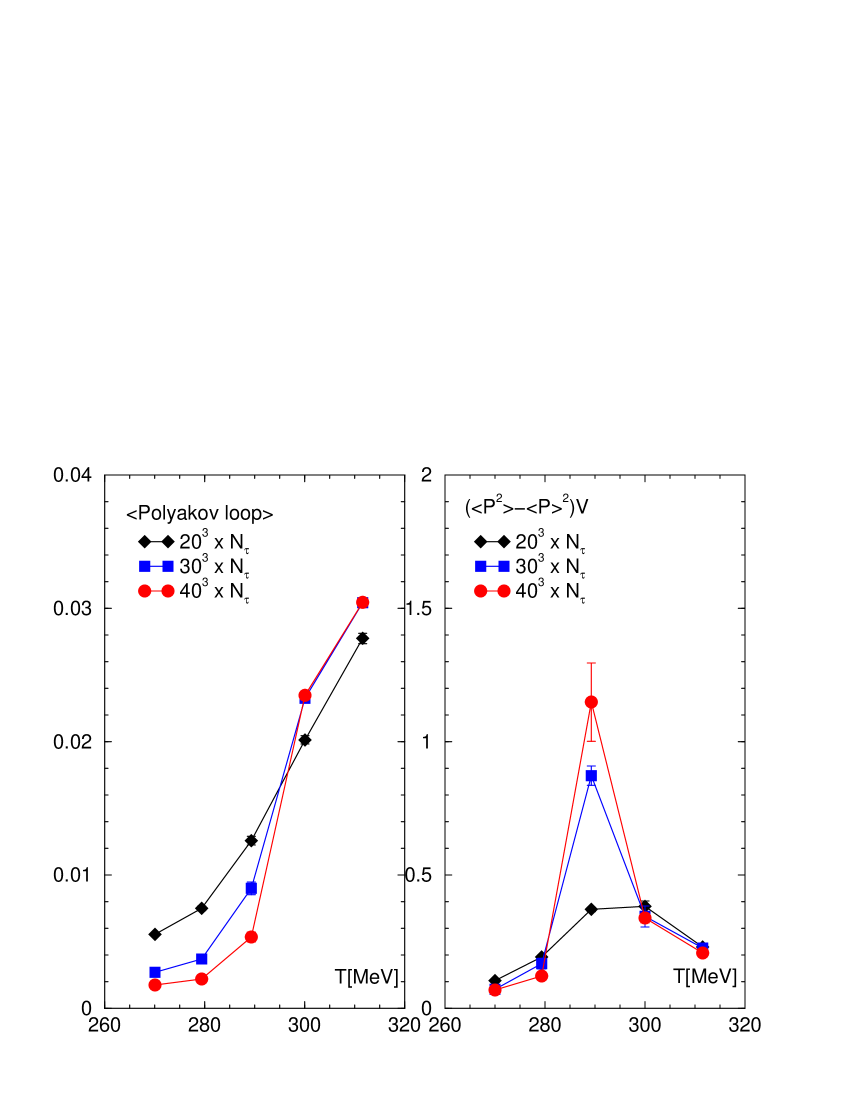
We calculate the Polyakov loop and its susceptibility on the anisotropic lattice. In addition to the lattices prepared for the EOS calculation, we generated different spatial volume lattices to study its finite size scaling. The parameters we adopted are listed in Table 2. Since the SU(3) gauge theory has the global Z(3) symmetry, we calculate the real part of Z(3)-rotated Polyakov loop and its susceptibility. Our results are shown in the left and center pannels of Fig.3. Unlike the case of conventional fixed studies, the renormalization factor is common to all temperatures. From the susceptibility data we can find that the transition point locates at corresponds to -300 MeV from the scale setting. We also find that the peak height of the susceptibility increases with increasing the system volume, in accordance with the 1st order nature of the transition.
| set | [fm] | [fm] | |||||
|---|---|---|---|---|---|---|---|
| a2-1 | 6.1 | 4 | 20 | 26-30 | 5.140(32) | 0.097 | 1.9 |
| a2-2 | 6.1 | 4 | 30 | 26-30 | 5.140(32) | 0.097 | 2.9 |
| a2-3 | 6.1 | 4 | 40 | 26-30 | 5.140(32) | 0.097 | 3.9 |
4 Static quark free energy
Finally, we study the static quark free energy in the fixed scale approach. In conventional fixed studies, the additive renormalization constant for is diffrent for each because the lattice spacing is different. Assuming that the short distance physics is independent of , the constant term is conventionally adjusted by hand such that around the smallest coinside with each other.
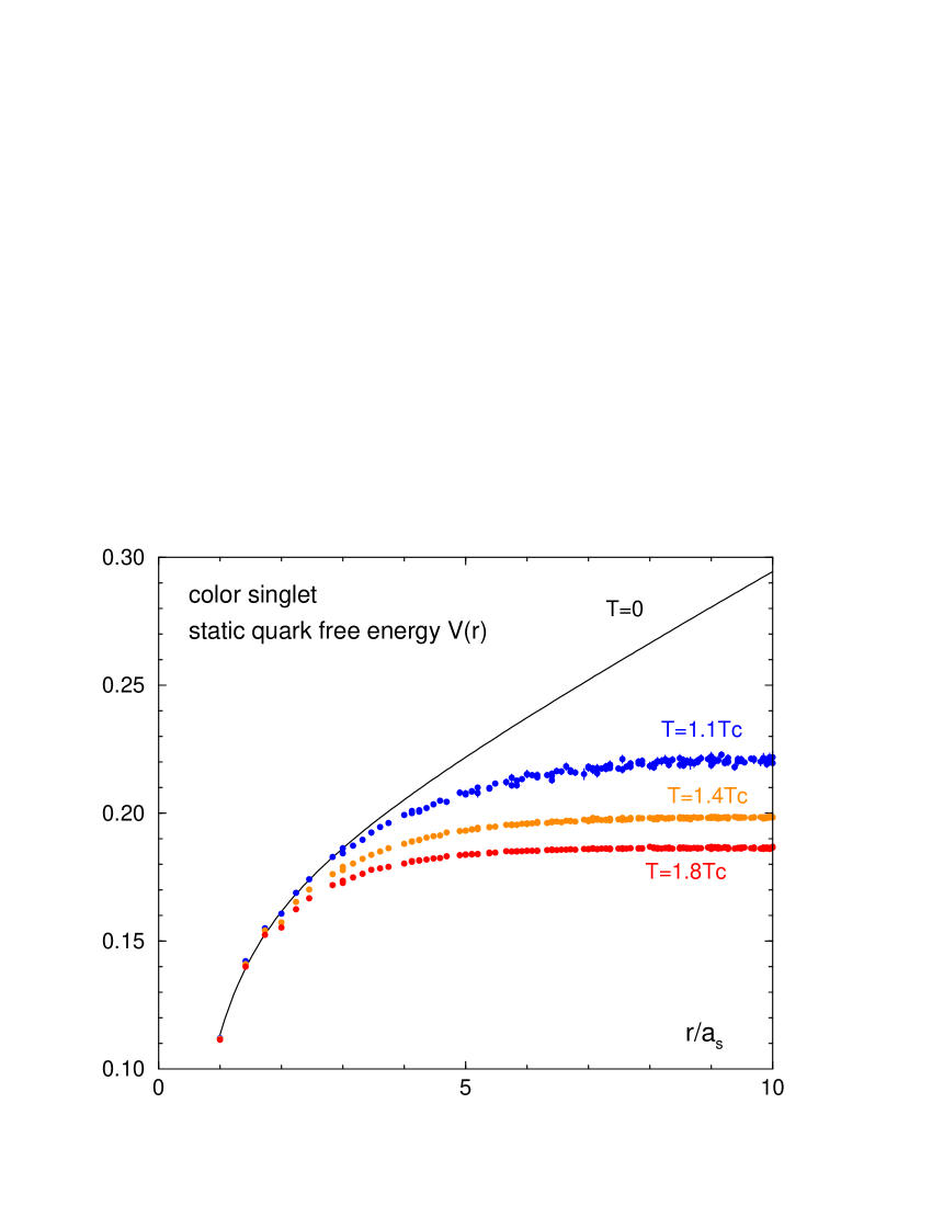
In the fixed scale approch, on the other hand, the common lattice spacing for all implies that the constant term in should be common too. Therefore, we can purely study the effects without adjusting the constant term. In Fig.3 (Right) we show our results of for the color singlet channel on the anisotropic lattice, without adjusting the constant term. The solid curve in the figure is a fit result of potential. We find that at different temperatures converge to a common curve at short distances. We thus have confirmed the expectation that the short distance physics is independent of .
5 Conclusions
We proposed a fixed scale approach to study the QCD thermodynamics on the lattice. In this approach, is varied by changing the temporal lattice size at a fixed lattice scale. To test the method, we applied it to the SU(3) gauge theory on isotropic and anisotropic lattices. We found that the -integral method to calculate the EOS works quite well. The main advantage of our approach is that the computational cost for simulations, which are the most time consuming calculations in the conventional fixed approaches, can be drastically reduced. We may even borrow configurations of existing high precision simulations at . The approach is applicable to QCD with dynamical quarks too. We are currently investigating EOS in flavor QCD with non-perturbatively improved Wilson quarks, using the configurations by the CP-PACS/JLQCD Collaboration [14]. With these fine lattices, the lattice artifacts around are much smaller than the conventional fixed approaches. We are further planning to use the PACS-CS configurations just at the physical point [15].
TU thanks H. Matusufuru for helpful discussions and comments. The simulations have been performed on supercomputers at RCNP, Osaka University and YITP, Kyoto University. This work is in part supported by Grants-in-Aid of the Japanese Ministry of Education, Culture, Sports, Science and Technology (Nos. 17340066, 18540253, 19549001, and 20340047). SE is supported by U.S. Department of Energy (DE-AC02-98CH10886).
References
- [1] C. DeTar, plenary talk at LATTICE 2008, to be published in PoS (LATTICE2008) 001.
- [2] J. Engels, J. Fingberg, F. Karsch, D. Miller and M. Weber, Phys. Lett. B 252, 625 (1990).
- [3] A. Ali Khan et al. [CP-PACS collaboration], Phys. Rev. D 64, 074510 (2001).
- [4] S. Aoki et al. [CP-PACS Collaboration and JLQCD Collaboration], Phys. Rev. D 73, 034501 (2006).
- [5] P. Chen et al., Phys. Rev. D 64, 014503 (2001).
- [6] T. Umeda et al. [WHOT-QCD collaboration], arXiv:0809.2842 [hep-lat].
- [7] T. Hirano, N. van der Kolk and A. Bilandzic, arXiv:0808.2684 [nucl-th].
- [8] R. G. Edwards, U. M. Heller and T. R. Klassen, Nucl. Phys. B 517, 377 (1998).
- [9] G. Boyd et al., Nucl. Phys. B 469, 419 (1996).
- [10] H. Matsufuru, T. Onogi and T. Umeda, Phys. Rev. D 64, 114503 (2001).
- [11] M. Okamoto et al. [CP-PACS Collaboration], Phys. Rev. D 60, 094510 (1999).
- [12] T. R. Klassen, Nucl. Phys. B 533, 557 (1998).
- [13] Y. Namekawa et al. [CP-PACS Collaboration], Phys. Rev. D 64, 074507 (2001).
- [14] T. Ishikawa et al. [JLQCD Collaboration], Phys. Rev. D 78, 011502 (2008).
- [15] Y. Kuramashi, plenary talk at LATTICE 2008, to be published in PoS (LATTICE2008) 018.