Infinite-randomness critical point in the two-dimensional disordered contact process

Abstract

We study the nonequilibrium phase transition in the two-dimensional contact process on a randomly diluted lattice by means of large-scale Monte-Carlo simulations for times up to $10^{10}$ and system sizes up to $8000\times 8000$ sites. Our data provide strong evidence for the transition being controlled by an exotic infinite-randomness critical point with activated (exponential) dynamical scaling. We calculate the critical exponents of the transition and find them to be universal, i.e., independent of disorder strength. The Griffiths region between the clean and the dirty critical points exhibits power-law dynamical scaling with continuously varying exponents. We discuss the generality of our findings and relate them to a broader theory of rare region effects at phase transitions with quenched disorder. Our results are of importance beyond absorbing state transitions because according to a strong-disorder renormalization group analysis, our transition belongs to the universality class of the two-dimensional random transverse-field Ising model.

I Introduction

Many-particle systems far from equilibrium can undergo phase transitions if external parameters are varied. These transitions, which separate different nonequilibrium steady states, are characterized by large-scale fluctuations and collective behavior over large distances and long times very similar to the behavior at equilibrium critical points. Examples of nonequilibrium phase transitions occur in a wide variety of systems ranging from surface chemical reactions and growing interfaces to traffic jams and to the spreading of epidemics in biology. Reviews of some of these transitions can be found, e.g., in Refs. Zhdanov and Kasemo (1994); Schmittmann and Zia (1995); Marro and Dickman (1999); Hinrichsen (2000a); Odor (2004); Lübeck (2004); Täuber et al. (2005)

In recent years, a large effort has been directed towards classifying possible nonequilibrium phase transitions Odor (2004). A particularly well-studied type of transitions separates active, fluctuating steady states from inactive absorbing states where fluctuations cease entirely. The generic universality class for these absorbing state transitions is directed percolation (DP) Grassberger and de la Torre (1979). According to a conjecture by Janssen and Grassberger Janssen (1981); Grassberger (1982), all absorbing state transitions with a scalar order parameter, short-range interactions, and no extra symmetries or conservation laws belong to this class. Examples include the transitions in the contact process Harris (1974a), catalytic reactions Ziff et al. (1986), interface growth Tang and Leschhorn (1992), or Pomeau’s conjecture regarding turbulence Pomeau (1986). In the presence of conservation laws or additional symmetries, other universality classes such as the parity conserving class or the $Z_{2}$-symmetric directed percolation (DP2) class can occur (see Ref. Hinrichsen (2000a) and references therein).

The DP universality class is ubiquitous in theory and computer simulations, but clearcut experimental verifications were lacking for a long time Hinrichsen (2000b). Partial evidence was manifest in the spatio-temporal intermittency in ferrofluidic spikes Rupp et al. (2003). Only very recently, a full verification (the only one, to the best of our knowledge) was found in the transition between two turbulent states in a liquid crystal Takeuchi et al. (2007). One possible cause for the surprising rarity of DP scaling in experiments are impurities, defects, or other kinds of disorder that are present in all realistic systems.

For this reason, the effects of quenched spatial disorder on the DP universality class have been studied for many years. However, a consistent picture has been very slow to emerge. According to the general Harris criterion Harris (1974b) (applied to the DP universality class by Kinzel Kinzel (1985) and Noest Noest (1986)), a clean critical point is (perturbatively) stable against weak spatial disorder, if the spatial correlation length critical exponent $\nu_{\perp}$ fulfills the inequality $d\nu_{\perp}>2$, where $d$ is the spatial dimensionality. The correlation length exponents of the DP universality class are $\nu_{\perp}\approx 1.097$ in one space dimension, 0.73 in two dimensions, and 0.58 in three dimensions Hinrichsen (2000a), therefore, the Harris criterion is violated in all dimensions $d<4$. The instability of the DP critical behavior against spatial disorder was confirmed by a field-theoretic renormalization group calculation Janssen (1997). This study did not produce a new critical fixed point but runaway flow towards large disorder, suggesting unconventional behavior . Early Monte-Carlo simulations in two space dimensions Moreira and Dickman (1996); Dickman and Moreira (1998) found logarithmically slow dynamics in violation of power-law scaling. Moreover, in analogy with Griffiths singularities Griffiths (1969), very slow dynamics was found in an entire parameter region near the transition Noest (1988); Bramson et al. (1991); Webman et al. (1998); Cafiero et al. (1998).

A crucial step towards resolving this puzzling situation was taken by Hooyberghs et al. Hooyberghs et al. (2003, 2004) who used the Hamiltonian formalism Alcaraz et al. (1994) to map the one-dimensional disordered contact process onto a random quantum spin chain. They then applied a Ma-Dasgupta-Hu strong-disorder renormalization group Ma et al. (1979); Igloi and Monthus (2005) and showed that the transition is controlled by an exotic infinite-randomness fixed point in the universality class of the random transverse-field Ising model Fisher (1992, 1995), at least for sufficiently strong disorder. This type of critical point displays ultraslow activated rather than power-law dynamical scaling. For weaker disorder, Hooyberghs et al. relied on numerical simulations and predicted non-universal continuously varying exponents, with either power-law or exponential dynamical scaling. Using large-scale Monte-Carlo simulations Vojta and Dickison Vojta and Dickison (2005) recently confirmed the infinite-randomness scenario. Moreover, their critical exponent values agreed with the predictions of the strong-disorder renormalization group (which can be solved exactly in one dimension), and they were universal, i.e., independent of disorder strength.

In higher dimensions, a strong-disorder renormalization group can still be applied, but, in contrast to one dimension, it cannot be solved analytically. By implementing the renormalization group numerically, Motrunich et al. Motrunich et al. (2000) demonstrated the existence of an infinite-randomness fixed point in two dimensions (and at least the flow towards larger disorder in three dimensions). However, reliable estimates for the critical exponent values have been hard to come by due to the small sizes available in the quantum simulations.

In this paper, we report the results of large-scale Monte-Carlo simulations of the contact process on two-dimensional randomly diluted lattices. The purpose of this work is twofold. First, we intend to determine beyond doubt the character and universality of the critical behavior; is it of conventional power-law type, infinite-randomness type or an even more exotic kind? Second, we intend to perform a careful data analysis that allows us to compute reasonably accurate exponent values. These will be important beyond the disordered contact process and apply to all systems controlled by the same infinite-randomness fixed point including the two-dimensional random transverse-field Ising magnet Motrunich et al. (2000).

The paper is organized as follows. In section II, we introduce our model, the contact process on a randomly diluted lattice. We then contrast the scaling theories for conventional critical points and infinite-randomness critical points. We also summarize the predictions for the Griffiths region. In section III, we present our simulation method and various numerical results together with a comparison to theory. We conclude in section IV by summarizing our findings, discussing three space dimensions, and relating our results to a broader classification of phase transitions with quenched disorder Vojta (2006).

II Model and phase transition scenarios

II.1 Contact process on a diluted lattice

The contact process Harris (1974a), a prototypical system in the DP universality class, can be interpreted as a simple model for the spreading of a disease. The clean contact process is defined on a $d$-dimensional hypercubic lattice. Each lattice site $\mathbf{r}$ can be active (infected) or inactive (healthy). In the course of the time evolution, active sites can infect their neighbors or they can spontaneously heal (become inactive). Specifically, the dynamics of the contact process is given by a continuous-time Markov process during which active sites become inactive at a rate $\mu$ while inactive site become active at a rate $\lambda n/(2d)$. Here, $n$ is the number of active nearest neighbor sites. The infection rate $\lambda$ and the healing rate $\mu$ (which can be set to unity without loss of generality) are external parameters. Their ratio controls the behavior of the system.

For $\lambda\ll\mu$, healing dominates, and the absorbing state without any active sites is the only steady state (inactive phase). For sufficiently large infection rate $\lambda$, there is a steady state with a nonzero density of active sites (active phase). These two phases are separated by a nonequilibrium phase transition in the DP universality class at a critical infection rate $\lambda_{c}^{0}$.

We now introduce quenched spatial disorder into the contact process by randomly diluting the underlying lattice. Specifically, we randomly remove each lattice site with probability $p$ . As long as the impurity concentration $p$ remains below the percolation threshold $p_{c}$, the lattice has an infinite connected cluster of sites which can support the active phase. Conversely, at dilutions above $p_{c}$, the lattice is decomposed into disconnected finite-size clusters. Because the infection eventually dies out on any finite cluster, there is no active phase for $p>p_{c}$. Consequently, the contact process on a randomly diluted lattice has two different nonequilibrium transitions (see also Fig. 1), the generic transition for $p<p_{c}$ which is driven by the dynamic fluctuations of the contact process and a percolation transition at $p=p_{c}$ which is driven by the lattice geometry Vojta and Lee (2006). The two transitions are separated by a multicritical point which was studied in Ref. Dahmen et al. (2007).

The basic observable in the contact process is the average density of active sites at time $t$,

$$\rho(t)=\frac{1}{L^{d}}\sum_{\mathbf{r}}\langle n_{\mathbf{r}}(t)\rangle$$ (1)

where $n_{\mathbf{r}}(t)=1$ if the site $\mathbf{r}$ is active at time $t$ and $n_{\mathbf{r}}(t)=0$ if it is inactive. $L$ is the linear system size, and $\langle\ldots\rangle$ denotes the average over all realizations of the Markov process. The longtime limit of this density (i.e., the steady state density)

$$\rho_{\rm stat}=\lim_{t\to\infty}\rho(t)$$ (2)

is the order parameter of the nonequilibrium phase transition.

II.2 Conventional power-law scaling

In this subsection, we briefly summarize the scaling theory for absorbing state transitions controlled by conventional fixed points with power-law dynamical scaling (see, e.g., Ref. Hinrichsen (2000a)), using the clean contact process as an example.

When the critical point $\lambda_{c}$ is approached from the active phase, the order parameter (steady state density) vanishes following the power law

$$\rho_{\rm stat}\sim(\lambda-\lambda_{c})^{\beta}\sim\Delta^{\beta}$$ (3)

where $\Delta=(\lambda-\lambda_{c})/\lambda_{c}$ is the dimensionless distance from the critical point, and $\beta$ is the order parameter critical exponent. In addition to the average density, we also need to characterize the length and time scales of the density fluctuations. When approaching the transition, the (spatial) correlation length $\xi_{\perp}$ diverges as

$$\xi_{\perp}\sim|\Delta|^{-\nu_{\perp}}~{}.$$ (4)

The correlation time $\xi_{\parallel}$ behaves like a power of the correlation length,

$$\xi_{\parallel}\sim\xi_{\perp}^{z},$$ (5)

i.e., the dynamical scaling is of power-law form. The three critical exponents $\beta$, $\nu_{\perp}$ and $z$ completely characterize the directed percolation universality class. The above relations allow us to write down the finite-size scaling form of the density as a function of $\Delta$, $t$, and $L$,

$$\rho(\Delta,t,L)=b^{\beta/\nu_{\perp}}\rho(\Delta b^{-1/\nu_{\perp}},tb^{z},Lb)~{},$$ (6)

where $b$ is an arbitrary dimensionless scale factor.

Two interesting observables can be studied if the time evolution starts from a single active site in an otherwise inactive lattice. The survival probability $P_{s}(t)$ is the probability that an active cluster survives at time $t$ when starting from such a single-site seed at time 0. For directed percolation, the survival probability scales exactly like the density ,

$$P_{s}(\Delta,t,L)=b^{\beta/\nu_{\perp}}P_{s}(\Delta b^{-1/\nu_{\perp}},tb^{z},Lb)~{}.$$ (7)

The pair connectedness function $C(\mathbf{r},t)=\langle n_{\mathbf{r}}(t)\,n_{0}(0)\rangle$ describes the probability that site $\mathbf{r}$ is active at time $t$ when starting from an initial condition with a single active site at $\mathbf{r}=0$ and time $0$. Because $C$ involves a product of two densities, its scale dimension is $2\beta/\nu_{\perp}$, and the full finite-size scaling form reads

$$C(\Delta,\mathbf{r},t,L)=b^{2\beta/\nu_{\perp}}C(\Delta b^{-1/\nu_{\perp}},\mathbf{r}b,tb^{z},Lb)~{}.$$ (8)

The total number of particles $N$ when starting from a single seed site can be obtained by integrating the pair connectedness $C$ over all space. This leads to the scaling form

$$N(\Delta,t,L)=b^{2\beta/\nu_{\perp}-d}N(\Delta b^{-1/\nu_{\perp}},tb^{z},Lb)~{}.$$ (9)

Finally, the mean-square radius $R$ of the active cluster, being a length, scales as

$$R(\Delta,t,L)=b^{-1}R(\Delta b^{-1/\nu_{\perp}},tb^{z},Lb)~{}.$$ (10)

At the critical point, $\Delta=0$, and in the thermodynamic limit, $L\to\infty$, the above scaling relations lead to the following predictions for the time dependencies of observables: The density and the survival probability asymptotically decay like

$$\rho(t)\sim t^{-\delta},\qquad P_{s}(t)\sim t^{-\delta}$$ (11)

with $\delta=\beta/(\nu_{\perp}z)$. In contrast, the radius and the number of particles in a cluster starting from a single seed site increase like

$$R(t)\sim t^{1/z},\qquad N(t)\sim t^{\Theta}$$ (12)

where $\Theta=d/z-2\beta/(\nu_{\perp}z)$ is the so-called critical initial slip exponent.

II.3 Activated scaling at an infinite-randomness fixed point

In this subsection we summarize the scaling theory for an infinite-randomness fixed point with activated scaling, as has been found in the one-dimensional disordered contact process Hooyberghs et al. (2003); Vojta and Dickison (2005); Vojta (2006).

At an infinite-randomness fixed point, the dynamics is ultraslow. The power-law dynamical scaling (5) gets replaced by activated scaling

$$\ln(\xi_{\parallel}/t_{0})\sim\xi_{\perp}^{\psi},$$ (13)

characterized by a new exponent $\psi$ called the tunneling exponent. (This name stems from the random transverse-field Ising model where this type of scaling was first found.) Here $t_{0}$ is a nonuniversal microscopic time scale. The exponential relation between time and length scales implies that the dynamical exponent $z$ is formally infinite. In contrast, the static scaling behavior remains of power law type.

Another important characteristic of an infinite-randomness fixed point is that the probability distributions of observables become extremely broad. Therefore, the average and typical value of an observable do not necessarily agree because averages may be dominated by rare events. Nonetheless, the scaling form of the average density at the infinite-randomness critical point is obtained by simply replacing the power-law scaling combination $tb^{z}$ by the activated combination $\ln(t/t_{0})b^{\psi}$ in the argument of the scaling function:

$$\rho(\Delta,\ln(t/t_{0}),L)=b^{\beta/\nu_{\perp}}\rho(\Delta b^{-1/\nu_{\perp}},\ln(t/t_{0})b^{\psi},Lb)~{}.$$ (14)

Analogously, the scaling forms of the average survival probability, the average number of sites in a cluster, and the mean-square cluster radius starting from a single site are

$$P_{s}(\Delta,\ln(t/t_{0}),L)=b^{\beta/\nu_{\perp}}P_{s}(\Delta b^{-1/\nu_{\perp}},\ln(t/t_{0})b^{\psi},Lb)$$ (15)

$$N(\Delta,\ln(t/t_{0}),L)=b^{2\beta/\nu_{\perp}-d}N(\Delta b^{-1/\nu_{\perp}},\ln(t/t_{0})b^{\psi},Lb).$$ (16)

$$R(\Delta,\ln(t/t_{0}),L)=b^{-1}R(\Delta b^{-1/\nu_{\perp}},\ln(t/t_{0})b^{\psi},Lb).$$ (17)

These activated scaling forms lead to logarithmic time dependencies at the critical point (in the thermodynamic limit). The average density and the survival probability asymptotically decay like

$$\rho(t)\sim[\ln(t/t_{0})]^{-\bar{\delta}},\qquad P_{s}(t)\sim[\ln(t/t_{0})]^{-\bar{\delta}}$$ (18)

with $\bar{\delta}=\beta/(\nu_{\perp}\psi)$ while the radius and the average number of particles in a cluster starting from a single seed site increase like

$$R(t)\sim[\ln(t/t_{0})]^{1/\psi},\qquad N(t)\sim[\ln(t/t_{0})]^{\bar{\Theta}}$$ (19)

with $\bar{\Theta}=d/\psi-2\beta/(\nu_{\perp}\psi)$.

In contrast to one dimension, where the critical exponents can be calculated exactly within the strong-disorder renormalization group, they need to be found numerically in higher dimensions.

II.4 Griffiths singularities

Quenched spatial disorder does not only destabilize the DP critical point, it also leads to interesting singularities, the so-called Griffiths singularities Griffiths (1969), in an entire parameter region around the transition. For a recent review of this topic at thermal, quantum, and nonequilibrium transitions, see Ref. Vojta (2006). In the context of the contact process on a diluted lattice, Griffiths singularities can be understood as follows.

Because lattice dilution reduces the tendency towards the active phase, the critical infection rate of the diluted system is higher than that of the clean system, $\lambda_{c}>\lambda_{c}^{0}$. For infection rates $\lambda$ with $\lambda_{c}>\lambda>\lambda_{c}^{0}$, the system is globally in the inactive phase, i.e., it eventually decays into the absorbing state. However, in the thermodynamic limit, one can find arbitrarily large spatial regions devoid of impurities. These rare regions are locally in the active phase. They cannot support a non-zero steady state density because they are of finite size, but their decay is very slow because it requires a rare, exceptionally large density fluctuation.

As a result, the inactive phase of the contact process on a diluted lattice can be divided into two regions. For infection rates below the clean critical point, $\lambda<\lambda_{c}^{0}$, the behavior is conventional. The system approaches the absorbing state exponentially fast in time. The decay time increases with $\lambda$ and diverges as $|\lambda-\lambda_{c}^{0}|^{-z\nu_{\perp}}$ where $z$ and $\nu_{\perp}$ are the exponents of the clean critical point Vojta and Dickison (2005); Dickison and Vojta (2005). Inside the Griffiths region, $\lambda_{c}>\lambda\geq\lambda_{c}^{0}$, one has to estimate the rare region contribution to the time evolution of the density Noest (1986, 1988). The probability $w$ for finding a rare region of linear size $L_{r}$ devoid of impurities is (up to pre-exponential factors) given by

$$w(L_{r})\sim\exp(-\tilde{p}L_{r}^{d})$$ (20)

with $\tilde{p}=-\ln(1-p)$. To exponential accuracy, the rare region contribution to the density can be written as

$$\rho(t)\sim\int dL_{r}~{}L_{r}^{d}~{}w(L_{r})\exp\left[-t/\tau(L_{r})\right]$$ (21)

where $\tau(L_{r})$ is the decay time of a rare region of size $L_{r}$. Let us first discuss the behavior at the clean critical point, $\lambda_{c}^{0}$, i.e., at the boundary between the conventional inactive phase and the Griffiths region. Here, the decay time of a single, impurity-free rare region of size $L_{r}$ scales as $\tau(L_{r})\sim L_{r}^{z}$ with $z$ the clean critical exponent [see (6)]. Using the saddle point method to evaluate the integral (21), we find the leading long-time decay of the density to be given by a stretched exponential,

$$\ln\rho(t)\sim-\tilde{p}^{z/(d+z)}~{}t^{d/(d+z)}~{},$$ (22)

rather than a simple exponential decay as for $\lambda<\lambda_{c}^{0}$.

Within the Griffiths region, $\lambda_{c}^{0}<\lambda<\lambda_{c}$, the decay time of a single rare region depends exponentially on its volume,

$$\tau(L_{r})\sim\exp(aL_{r}^{d})$$ (23)

because a coordinated fluctuation of the entire rare region is required to take it to the absorbing state Noest (1986, 1988); Schonmann (1985). The nonuniversal prefactor $a$ vanishes at the clean critical point $\lambda_{c}^{0}$ and increases with $\lambda$. Close to $\lambda_{c}^{0}$, it behaves as $a\sim\xi_{\perp}^{-d}\sim(\lambda-\lambda_{c}^{0})^{d\nu_{\perp}}$ with $\nu_{\perp}$ the clean critical exponent. Repeating the saddle point analysis of the integral (21) for this case, we obtain a power-law decay of the density

$$\rho(t)\sim t^{-\tilde{p}/a}=t^{-d/z^{\prime}}$$ (24)

where $z^{\prime}=da/\tilde{p}$ is a customarily used nonuniversal dynamical exponent in the Griffiths region. Its behavior close to the dirty critical point $\lambda_{c}$ can be obtained within the strong disorder renormalization group method Hooyberghs et al. (2004); Fisher (1995); Motrunich et al. (2000). When approaching the phase transition, $z^{\prime}$ diverges as

$$z^{\prime}\sim|\lambda-\lambda_{c}|^{-\psi\nu_{\perp}}$$ (25)

where $\psi$ and $\nu_{\perp}$ are the exponents of the dirty critical point.

Let us emphasize that strong power-law Griffiths singularities such as (24) usually occur in connection with infinite-randomness critical points, while conventional critical points display exponentially weak Griffiths effects Vojta (2006). Thus, the character of the Griffiths singularities can be used to identify the correct scaling scenario.

III Monte-Carlo simulations

III.1 Method and overview

We now turn to the main objective of our work, large-scale Monte-Carlo simulations of the contact process on a randomly diluted square lattice. There are several efficient computational implementations of the contact process, all equivalent with respect to the universal behavior at the phase transition. We followed the algorithm described, e.g., by Dickman Dickman (1999). The simulation starts at time $t=0$ from some configuration of active and inactive sites. Each event consists of randomly selecting an active site $\mathbf{r}$ from a list of all $N_{a}$ active sites, selecting a process: creation with probability $\lambda/(1+\lambda)$ or annihilation with probability $1/(1+\lambda)$ and, for creation, selecting one of the four neighboring sites of $\mathbf{r}$. The creation succeeds, if this neighbor is empty (and not an impurity site). The time increment associated with this event is $1/N_{a}$.

Using this method, we investigated systems with sizes of up to $8000\times 8000$ sites and impurity (vacancy) concentrations $p=0$, 0.1, 0.2, 0.3, and $p=p_{c}=0.407254$. To explore the ultraslow dynamics predicted in the infinite-randomness scaling scenario, we simulated very long times up to $t=10^{10}$ which is, to the best of our knowledge, significantly longer than all previous simulations of the disordered two-dimensional contact process. In all cases, we averaged over many disorder realizations, details will be mentioned below for each specific simulation. The total numerical effort was approximately 40000 CPU-days on the Pegasus Cluster at Missouri S&T.

To identify the critical point for each parameter set, and to determine the critical behavior, we carried out two types of simulations, (i) runs starting from a completely active lattice during which we monitor the time evolution of the density $\rho(t)$, and (ii) runs starting from a single active site in an otherwise inactive lattice during which we monitor the survival probability $P_{s}(t)$ and the size $N_{s}(t)$ of the active cluster. Figure 1 gives an overview of the phase diagram resulting from these simulations. As expected, the critical infection rate $\lambda_{c}$ increases with increasing impurity concentration. In the following subsections we discuss the behavior in the vicinity of the phase transition in more detail.

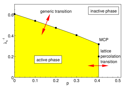
Figure 1: (Color online) Phase diagram of the contact process on a site-diluted square lattice (inverse critical infection rate $\lambda_{c}^{-1}$ vs impurity concentration $p$). MCP marks the multicritical point. The black dots show the actual simulation results, the lines are guides to the eye.

III.2 Clean 2d contact process

We first performed a number of simulations for clean undiluted lattices ($p=0$), mainly to test our numerical implementation of the contact process. Fig. 2 shows the density $\rho(t)$ for runs starting from a completely active lattice. The data are averages over 60 runs of a system of linear size $L=4000$ except for the two infection rates closest to the transition, $\lambda=1.64874$ and 1.64875 for which we performed 42 runs of a system of size $L=8000$.

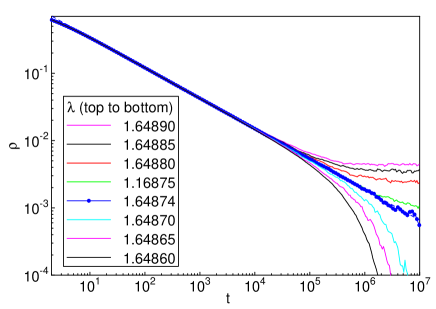
Figure 2: (Color online) Time evolution of the average density $\rho(t)$ for the contact process on an undiluted ($p=0$) square lattice, starting from a completely active lattice.

From these simulations, we estimate the critical infection rate to be $\lambda_{c}^{0}=1.64874(2)$ where the number in brackets gives the error of the last digit. The critical exponent $\delta$ can be determined from a power-law fit of $\rho(t)$; we find $\delta=0.4526(7)$.

We then perform a scaling analysis of $\rho(t)$ [based on (6)] on the inactive side of the transition using 12 different infection rates between 1.60 and $\lambda_{c}^{0}=1.64874$. This allows us to find the exponent combination $z\nu_{\perp}=1.290(4)$. Finally, we carried out several runs right at the critical point but with system sizes varying from $L=25$ to $L=8000$. A finite-size scaling analysis [again based on (6)] gives the dynamical exponent $z=1.757(8)$. All other critical exponents can now be calculated from the scaling relations (6), (7), and (9). We find $\nu_{\perp}=0.734(6)$, $\beta=0.584(3)$, and $\Theta=0.233(6)$.

To verify the results we also carried out simulations starting from a single active seed site. Using 500,000 runs with a maximum time of $10^{6}$, we arrived at the same value $\lambda_{c}^{0}=1.64874(2)$ for the critical infection rate. We measured the survival probability $P_{s}(t)$, the number of active sites $N_{s}(t)$ and the mean square radius of the active cluster $R(t)$. The resulting estimates of the exponents $\delta$, $\Theta$, and $z$ confirmed the values quoted above.

Our results are in excellent agreement with, and of comparable accuracy to, other large-scale simulation of the DP universality class in two dimensions (see, e.g., Ref. Dickman (1999) and references therein).

III.3 Diluted 2d contact process: Overview

We start our discussion of the diluted contact process by showing in Fig. 3 an overview of the survival probability $P_{s}(t)$ for a system with impurity concentration $p=0.2$, covering the $\lambda$ range from the conventional inactive phase, $\lambda<\lambda_{c}^{0}$, all the way to the active phase, $\lambda>\lambda_{c}$.

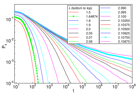
Figure 3: (Color online) Time evolution of the survival probability $P_{s}(t)$ for impurity concentration $p=0.2$, starting from a single seed site. The clean critical infection rate $\lambda_{c}^{0}=1.64874$ and the actual critical point $\lambda_{c}=2.10750$ are specially marked.

The data represent averages over 5000 disorder configurations, with 128 runs for each disorder configuration starting from random seed sites. The system size, $L=2000$, is chosen such that the active cluster stays much smaller then the sample over the time interval of the simulation (thus eliminating finite-size effects).

For infection rates below and at the clean critical point $\lambda_{c}^{0}=1.64874$, the density decay is very fast, clearly faster than a power law. Above $\lambda_{c}^{0}$, the decay becomes slower and asymptotically appears to follow a power law with an exponent that varies continuously with $\lambda$. For even larger infection rates, the decay seems to be slower than a power law. At the largest infection rates, the system will ultimately reach a nonzero steady-state survival probability, i.e., the it is in the active phase.

Let us emphasize that the behavior in Fig. 3, in particular, the nonuniversal power-law decay over a range of infection rates, already provides support for the infinite-randomness scenario of subsection II.3 while it disagrees with the conventional scenario (subsection II.2) of power-law behavior restricted to the critical point and exponentially weak Griffiths effects.

III.4 Finding the critical point

A very efficient method for identifying the critical point in the clean contact process and other clean reaction-diffusion systems is to look for the critical power-law time dependencies of various observables. To use the same idea in our diluted contact process simulations, we plot $\ln P_{s}(t)$, $\ln N_{s}(t)$ and $\ln\rho(t)$ versus $\ln\ln t$. In such plots, the anticipated logarithmic laws (18) and (19) correspond to straight lines. Figure 4 shows these plots for several infection rates close to the critical point.

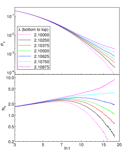
Figure 4: (Color online) $\ln P_{s}(t)$ and $\ln N_{s}(t)$ versus $\ln\ln t$ for several infection rates close to the critical point (at least 5000 disorder realizations with 128 trials each, $p=0.2$).

The parameters are as in subsection III.3. At the first glance, the data at the appropriate critical infection rate appear to follow the expected logarithmic behavior over several orders of magnitude in time $t$. However, a closer inspection reveals a serious problem. The survival probability $P_{s}$ suggests a critical infection rate $\lambda_{c}$ in the range 2.10500 to 2.10625 while the cluster size $N_{s}$ appears subcritical even at the larger value 2.10750. Such a discrepancy suggests strong corrections to scaling.

The origin of these corrections can be easily understood by rewriting $P_{s}(t)\sim[\ln(t/t_{0})]^{-\bar{\delta}}=[\ln(t)-\ln(t_{0})]^{-\bar{\delta}}$. The microscopic time scale thus provides a correction to scaling; and since we cover only a moderate range in $\ln(t)$, it strongly influences the results. We emphasize that this problem is intrinsic to the case of activated scaling (and thus unavoidable) because logarithms, in contrast to power laws, are not scale free. Identifying straight lines in plots like Fig. 4 is thus not a reliable tool for finding the critical point, even more so because simulations in 1D (where the analysis is much easier because the critical exponents are known exactly) have given sizable $t_{0}\approx 100\ldots 500$ for typical parameter values Vojta and Dickison (2005).

To circumvent this problem, we devised a method for finding the critical point without needing a value for the microscopic scale $t_{0}$. It is based on the observation that in the infinite-randomness scenario, $t_{0}$ has the same value in the scaling forms of all observables (because it is related to the basic energy scale of the strong-disorder renormalization group). Thus, if we plot $N_{s}(t)$ versus $P_{s}(t)$, the critical point corresponds to power-law behavior provided all other corrections to scaling are weak. The same is true for other combinations of observables.

Figure 5 shows a plot of $N_{s}(t)$ versus $P_{s}(t)$ for several infection rates close to the phase transition.

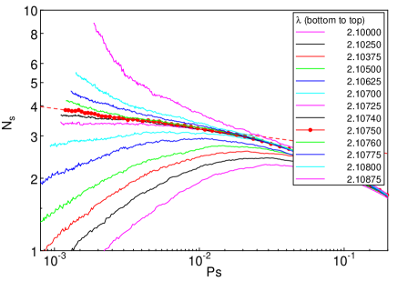
Figure 5: (Color online) $\ln N_{s}(t)$ versus $\ln P_{s}(t)$ and for several infection rates close to the critical point. The straight line is a power-law fit of the asymptotic part of the $\lambda=2.10750$ curve. ($p=0.2$, 5000 - 20,000 disorder realizations with 128 trials each.

The figure shows that the data for $\lambda=2.1075$ follow the expected power law for about a decade in $P_{s}$ ($10^{-3}<P_{s}<10^{-2}$, corresponding to 4 decades of time, from about $10^{4}$ to $10^{8}$), while the data at higher and lower $\lambda$ curve away as expected. We therefore identify $\lambda_{c}=2.1075(1)$ as the critical infection rate for dilution $p=0.2$. This value agrees well with an estimate based on Dickman’s Moreira and Dickman (1996) heuristic criteria of $\lambda_{c}$ being the smallest $\lambda$ supporting asymptotic growth of $N_{s}(t)$.

Figure 5 also reveals two remarkable features of the problem. (i) The asymptotic critical region is extremely narrow, $|\Delta|=|\lambda-\lambda_{c}|/\lambda_{c}\lessapprox 10^{-3}$, at least for these two observables. This follows from fact that the data for $\lambda$ outside the small interval [2.1070, 2.1080] curve away from the critical curve well before it reaches the asymptotic regime. (ii) The crossover to the asymptotic behavior occurs very late since $P_{s}\approx 0.01$ corresponds to a crossover time of $t_{x}\approx 10^{4}$, implying that very long simulations are necessary to extract the true critical behavior. Moreover, the mean-square radius of a surviving active cluster at the crossover time is $R(t_{x})\approx 55$, corresponding to an overall diameter of about 200. This means simulations with linear system sizes below about 200 will never reach the asymptotic behavior. We confirmed this observation by carrying out simulations with smaller sizes.

Having determined the critical point, we can now obtain a rough estimate of the microscopic time scale $t_{0}$ by replotting $\ln P_{s}(t)$ and $\ln N_{s}(t)$ as functions of $\ln\ln(t/t_{0})$ with varying $t_{0}$. At the correct value for $t_{0}$, the critical curves ($\lambda=2.1075$) of all observables must be straight lines. By performing this analysis for $P_{s}(t)$, $N_{s}(t)$, and $\rho(t)$ we find $\ln t_{0}=5.5\pm 1.0$ for dilution $p=0.2$. The results for all the observables agree within the error bars, providing an additional consistency check for our method and the underlying infinite-randomness scenario.

III.5 Critical behavior

According to subsection II.3, the critical behavior at the infinite-randomness fixed point can be characterized by three independent exponents, e.g., $\beta$, $\nu_{\perp}$, and $\psi$. The two “static” exponents $\beta$ and $\nu_{\perp}$ can in principle be determined without reference to $t_{0}$, the value of the tunneling exponent $\psi$ depends on the above estimate for $t_{0}$.

The combination $\beta/\nu_{\perp}$ (the scale dimension of the order parameter) can be obtained directly from the critical curve in Fig. 5. By combining eqs. (18) and (19), we find $N_{s}\sim P_{s}^{-\bar{\Theta}/\bar{\delta}}\sim P_{s}^{2(1-\nu_{\perp}/\beta)}$. A fit of the asymptotic part of the critical curve gives $\beta/\nu_{\perp}=0.96(2)$. Here, the error is almost entirely due to the uncertainty in locating the critical infection rate $\lambda_{c}$, the statistical error is much smaller. We obtained independent estimates for $\beta/\nu_{\perp}$ from analyzing plots of $N_{s}$ vs. $R$ and $P_{s}$ vs. $R$ in a similar fashion. The results agree with the above value within their error bars.

To obtain the tunneling exponent $\psi$, we now fit the critical survival probability $P_{s}(t)$ to $[\ln(t/t_{0})]^{-\bar{\delta}}$ (for times up to $t=10^{8}$) using our estimate $\ln t_{0}=5.5\pm 1.0$. We find $\bar{\delta}=1.9(2)$ with the error mainly coming from the uncertainties in $\lambda_{c}$ and $t_{0}$. An analogous analysis of the density of active sites $\rho(t)$ in a simulation starting from a fully infected lattice ($L=8000$, times up to $t=10^{9}$) gives exactly the same value (see Fig. 6).

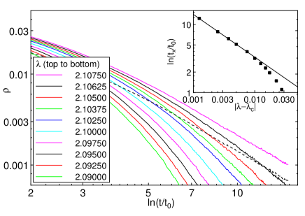
Figure 6: (Color online) $\ln\rho(t)$ versus $\ln\ln(t/t_{0})$ and for several infection rates at and below to the critical point. The dashed line represents 2/3 of the critical $\rho$. Inset: Time $t_{x}$ at which the density falls below 2/3 of the critical value as a function of the distance from criticality. The solid line is a power-law fit of $\ln(t_{x}/t_{0})$ vs $\Delta$. ($p=0.2$, 13 disorder realizations with $L=8000$ for $\lambda>2.1$, 250 realizations with $L=2000$ for $\lambda\leq 2.1$)

From the time evolution of $N_{s}(t)$, we also find the estimate $\bar{\Theta}=0.15(3)$ for the initial slip exponent. Using $\psi=\beta/(\nu_{\perp}\bar{\delta})$ gives the tunneling exponent, $\psi=0.51(6)$. Estimates obtained from $N_{s}(t)$ and directly from fitting $R(t)$ to $[\ln(t/t_{0})]^{1/\psi}$ agree within the error bars with this value. It must be emphasized that the value of $\psi$ sensitively depends on the correct identification of $t_{0}$. A naive fit of $P_{s}(t)$ to a power of $\ln(t)$ would give a value of about 3.0 for $\bar{\delta}$ and thus a much smaller value of about 0.33 for $\psi$.

Finding the final missing exponent in our triple ($\beta$, $\nu_{\perp}$, $\psi$) requires the analysis of off-critical simulation runs. Here, the extreme narrowness of the asymptotic critical region causes serious problems, because we have only three $\lambda$ values from 2.1070 to $\lambda_{c}=2.1075$. Moreover, a glance at Fig.  5 shows that adding simulations runs at additional $\lambda$ closer to the critical point would only make sense if we also significantly increased the simulation time and/or the number of disorder realizations. Because this appears to be beyond our present computational capabilities, we determine an estimate for $\beta$ by extrapolating the effective exponent obtained outside the asymptotic critical region. To this end, we analyze the time evolution of the density $\rho(t)$ starting from a fully infected lattice show in Fig.  6 for various infection rates $\lambda$ below the critical point. For each $\lambda$, we define a crossover time $t_{x}$ at which the density $\rho(t)$ is exactly 2/3 of the critical density at the same time.

This crossover time can be analyzed in two ways. According to (14), it should behave as $\ln(t_{x}/t_{0})\sim|\Delta|^{-\nu_{\perp}\psi}$. The inset of Fig.  6 shows a fit to this form, giving $\nu_{\perp}\psi=0.64(10)$. However, this value depends on our estimate for the microscopic scale $t_{0}$. To avoid relying on $t_{0}$, we plot $|\Delta(t_{x})|$ vs. the critical $\rho(t)$ (at $t=t_{x}$) in Fig. 7.

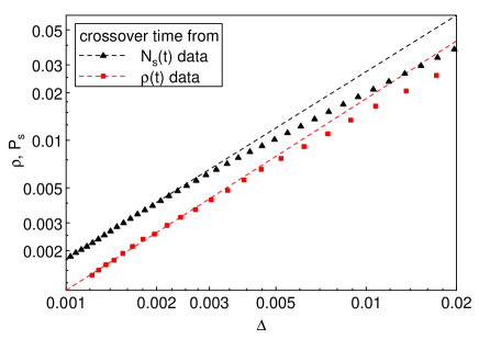
Figure 7: (Color online) $\ln\rho(t)$ vs. $\ln\Delta(t)$ at the crossover time $t=t_{x}$ for the density itself and $\ln P_{s}(t)$ vs. $\ln\Delta(t)$ at the crossover time $t=t_{x}$ for the particle number $N_{s}$. The dashed lines are power-law fits to the expected behavior $\rho\sim P_{s}\sim|\Delta|^{\beta}$.

According to (14), the expected behavior is a power law $\rho\sim|\Delta|^{\beta}$. The same analysis can also be performed by analyzing the crossover of $N_{s}(t)$ and plotting the resulting $\Delta(t_{x})$ vs. $P_{s}(t)$. Both data sets show significant curvature (i.e. deviations from the expected power law behavior) which is not surprising because the underlying $\lambda$ are not in the asymptotic region. By fitting the small-$\Delta$ part of both curves, we estimate $\beta=1.15(15)$. A fit of $\Delta(t_{x})$ vs. $N_{s}(t)$ gives $\nu_{\perp}-\beta=0.045(15)$. Thus, our final estimate for the correlation length exponent $\nu_{\perp}=1.20(15)$ in agreement with the Harris criterion $\nu_{\perp}\geq 2/d=1$.

III.6 Universality

The universality of the infinite-randomness scenario for the critical point in the disordered contact process has been controversially discussed in the past Hooyberghs et al. (2004); Vojta and Dickison (2005); Neugebauer et al. (2006). The underlying strong-disorder renormalization group becomes exact only in the limit of broad disorder distributions and can thus not directly address the fate of a weakly disordered system. However, Hoyos Hoyos (2008) recently showed that within this renormalization group scheme, the disorder always increases under renormalization, even if it is weak initially. Moreover, the perturbative renormalization group of Janssen Janssen (1997), which is controlled for weak disorder, displays runaway flow towards large disorder strength supporting a universal scenario in which the infinite-randomness fixed point controls the transition for all bare disorder strength.

To address this question in our simulations, we repeat the above analysis for impurity concentrations $p=0.1$ and 0.3 albeit with somewhat smaller numbers of disorder realizations. We determine the critical infection rates from plots of $N_{s}(t)$ vs. $P_{s}(t)$ analogous to Fig. 5 and find $\lambda_{c}=1.8462(3)$ for $p=0.1$ and $\lambda_{c}=2.4722(2)$ for $p=0.3$. Figure 8 shows the critical $N_{s}$ vs. $P_{s}$ curves for $p=0.1$, 0.2, and 0.3.

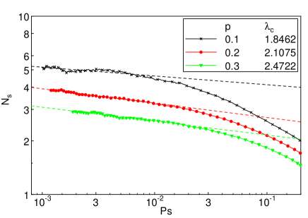
Figure 8: (Color online) $\ln N_{s}(t)$ versus $\ln P_{s}(t)$ at criticality for impurity concentrations $p=0.1$, 0.2, and 0.3. The dashed lines are power-law fits of the asymptotic parts (18000 disorder configurations for $p=0.2$, 4000 each for $p=0.1$ and 0.3, 128 spreading trials for each configuration).

In the long-time (low-$P_{s}$) limit, all three curves follow power-laws, and the resulting values for the exponent $\beta/\nu_{\perp}$ agree within their error bars, $\beta/\nu_{\perp}=0.97(3)$ for $p=0.1$, $\beta/\nu_{\perp}=0.96(2)$ for $p=0.2$, and $\beta/\nu_{\perp}=0.96(3)$ for $p=0.3$.

Having fixed the critical point for all $p$, we determine the microscopic time scale $t_{0}$ as in subsection III.4. Its value changes significantly with $p$, it is $\ln t_{0}\approx 6.5$ (for $p=0.1$), 5.5 (for $p=0.2$), and 4.0 (for $p=0.3$). Power-law fits of $P_{s}(t)$ and $N_{s}(t)$ to $\ln(t/t_{0})$ give estimates for the exponents $\bar{\delta}$ and $\bar{\Theta}$. Within their error bars, the values for $p=0.1$ and 0.3 agree with the respective values for $p=0.2$ discussed in subsection III.5.

Our simulations thus provide numerical evidence for the critical behavior of the disordered 2D contact process being universal, i.e., being controlled by the same infinite-randomness fixed point for all disorder strength. Note that the bare disorder can be considered weak for $p=0.1$ as the difference of the critical infection rate from its clean value is small, $(\lambda_{c}-\lambda_{c}^{0})/\lambda_{c}^{0}\approx 0.12$.

III.7 Griffiths region

In addition to the critical point, we have also studied the Griffiths region $\lambda_{c}^{0}<\lambda<\lambda_{c}$ in some detail. Figure 9 shows a double-logarithmic plot of the density $\rho(t)$ (starting from a fully infected lattice) for several infection rates in this region.

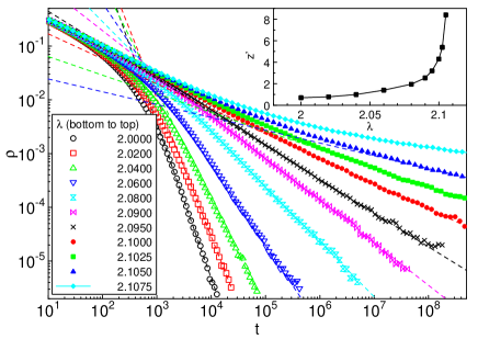
Figure 9: (Color online) $\ln\rho(t)$ versus $\ln t$ for several infection rates in the Griffiths region, $\lambda_{c}^{0}<\lambda<\lambda_{c}$ ($p=0.2$, 13 disorder realizations with $L=8000$ for $\lambda>2.1$, 250 realizations with $L=2000$ for $\lambda\leq 2.1$ ). The dashed lines are power-law fits of the long-time behavior to (24). Inset: Resulting dynamical exponent $z^{\prime}$ as a function of $\lambda$.

For all these $\lambda$, the long-time behavior of the density follows the expected power law over several order of magnitude in time and/or density. The values of the (non-universal) dynamical exponent $z^{\prime}$ can be determined by fitting the long-time behavior to eq. (24). The inset of Fig. 9 shows that $z^{\prime}$ diverges with $\lambda$ approaching the critical point $\lambda_{c}=2.1075$. Fitting this divergence to the power law (25) expected within the infinite-randomness scenario, we find $\psi\nu_{\perp}\approx 0.61$ in good agreement with the value extracted from the scaling analysis of the density in subsection III.5. Performing the same analysis with the survival probability data shown in Fig. 3 gives analogous results.

III.8 Spatial correlations

To study the spatial correlations in the diluted contact process close to criticality, we calculate the average equal-time correlation function $G=\frac{1}{N}\sum_{\mathbf{r}}\langle n_{\mathbf{r}}(t)n_{0}(t)\rangle$ from the late-time configurations arising in the simulations starting from a fully infected lattice. Scaling arguments analogous to those leading to (8) suggest the scaling form

$$G(\Delta,\mathbf{r},\ln(t/t_{0}))=b^{2\beta/\nu_{\perp}}G(\Delta b^{-1/\nu_{\perp}},\mathbf{r}b,\ln(t/t_{0})b^{\psi})~{}.$$ (26)

To find the true stationary behavior of $G$, one would ideally want to sample the quasistationary state which is not directly available from our simulations for $\lambda\leq\lambda_{c}$. However, the finite-time data allow us to extract the short-distance behavior up to a crossover distance $r_{x}(t)$ given by the scaling combination $\ln(t/t_{0})r_{x}^{-\psi}\gtrsim 1$. Figure 10 shows the correlation function for infection rates close to the critical point.

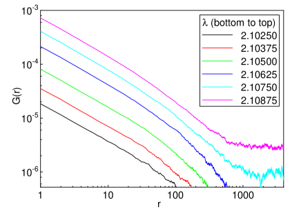
Figure 10: (Color online) $\ln G(r)$ vs. $\ln r$ for several infection rates $\lambda$ ($p=0.2$, 13 disorder realizations with $L=8000$). $G(r)$ is calculated from the configurations at late times of the time evolution ($t\geq 4\times 10^{8}$).

The data show a crossover at a length scale of about 200 compatible with the crossover scale identified at the end of Section III.4 separating the pre-asymptotic behavior from the true asymptotic long-distance form. Unfortunately, we cannot explore the asymptotic region because (i) fluctuations are too strong, and (ii) for larger distances, we violate the condition $\ln(t/t_{0})r_{x}^{-\psi}\gtrsim 1$ discussed above. Thus, the asymptotic functional form of the spatial correlation function remains a task for the future.

III.9 Nonequilibrium transition across the lattice percolation threshold

So far, we have considered the generic transition occurring for impurity concentrations $p<p_{c}$. In the present subsection, we briefly discuss the nonequilibrium phase transition of the contact process across the percolation threshold $p_{c}$ of the underlying lattice. It occurs at sufficiently large infection rates and is represented by the vertical line at $p_{c}$ in the phase diagram shown in Fig. 1.

Vojta and Lee Vojta and Lee (2006) developed a theory for this transition by combining the well-known critical behavior of classical percolation with the properties of a supercritical contact process on a finite-size cluster. They found that the behavior of the contact process on a diluted lattice close to the percolation threshold follows the activated scaling scenario of subsection II.3. However, the critical exponents differ from those of the generic transition discussed above; they can be expressed as combinations of the classical lattice percolation exponents $\beta_{c}$ and $\nu_{c}$ which are known exactly in two space dimensions. Specifically, the static exponents $\beta$ and $\nu_{\perp}$ are identical to their lattice counterparts $\beta=\beta_{c}=5/36$ and $\nu_{\perp}=\nu_{c}=4/3$. The tunneling exponent $\psi$ is given by $\psi=D_{c}=2-\beta_{c}/\nu_{c}=91/48$ where $D_{c}$ is the fractal dimension of the critical percolation cluster (of the lattice). This implies an extremely small value for the exponent controlling the critical density decay, $\bar{\delta}=\beta/(\nu_{\perp}\psi)=5/91$.

To test this prediction, we performed simulation runs at $p=p_{c}$ and $\lambda=5.0$, starting from a fully infected lattice. The resulting time evolution of the density of active sites (averaged over three samples of linear size $L=8000$) is presented in Figure 11.

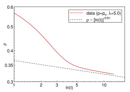
Figure 11: (Color online) $\ln\rho(t)$ versus $\ln\ln(t)$ for $p=p_{c}$, $\lambda=5.0$, and $L=8000$. We have simulated 3 samples, their differences are smaller than the line width. The dashed line represents the expected logarithmic long-time decay, $\rho\sim[\ln(t)]^{-\bar{\delta}}$ with arbitrary prefactor.

The data show the behavior predicted in Ref. Vojta and Lee (2006): a rapid initial density decay towards a quasi-stationary density, followed by a slow logarithmic time dependence due to the successive decays of the contact process on larger and larger percolation clusters. The asymptotic behavior is compatible with the predicted exponent value $\bar{\delta}=5/91$, however, determining an accurate value of $\bar{\delta}$ from the simulation data is impossible because of the extremely slow decay and the limited time range we can cover.

IV Discussion and conclusions

In this final section of the paper, we summarize our results and discuss some aspects of our data analysis. We then briefly consider the diluted contact process in three space dimensions. Finally, we relate our findings to a recent classification of phase transitions with weak disorder.

IV.1 Summary

We have performed large-scale Monte-Carlo simulations of the contact process on a two-dimensional site-diluted lattice. We have determined the infection-dilution phase diagram und studied both the generic nonequilibrium phase transition for dilutions below the percolation threshold of the lattice and the transition across the lattice percolation threshold.

Our main results is that the generic transition is controlled by an infinite-randomness fixed point for all disorder strength investigated, giving rise to ultraslow activated rather than power-law dynamical scaling. Based on two types of simulations, (i) spreading of the infection from a single seed and (ii) simulations starting from a fully infected lattice, we have determined the complete critical behavior. Our critical exponent values are summarized in Table 1.

critical exponent	value	value
	(generic)	(percolation)
$\beta/\nu_{\perp}$	0.96(2)	5/48
$\beta$	1.15(15)	5/36
$\nu_{\perp}$	1.20(15)	4/3
$\psi$	0.51(6)	91/48
$\bar{\delta}$	1.9(2)	5/91
$\bar{\Theta}$	0.15(3)

Table 1: Critical exponents for the nonequilibrium phase transitions of the disordered two-dimensional contact process. The values for the generic transition are from this work, the values for the percolation transition are from Ref. Vojta and Lee (2006). The numbers in brackets give an error estimate of the last given digits.

Note that the spatial correlation length exponent fulfills the Harris criterion Harris (1974b) inequality $d\nu_{\perp}\geq 2$, as expected in a disordered system Chayes et al. (1986).

We have been able to obtain a rather accurate estimate for the finite-size scaling exponent $\beta/\nu_{\perp}$. However, the other exponents are somewhat less accurate despite our extensive numerical effort (system sizes up to 8000$\times$8000 sites and times up to $10^{10}$). This is caused by three important characteristics of our infinite-randomness critical point:

(i) The logarithmic time-dependencies associated with activated scaling are not scale-free, they contain a microscopic time scale $t_{0}$ which acts as a strong correction to scaling and must be estimated independently (otherwise the exponent values will be seriously compromised). Since our simulations cover only a limited range of $\ln(t)$, our values for $t_{0}$ are not very precise which limits the accuracy of the exponents $\bar{\delta}$, $\bar{\Theta}$, and $\psi$.

(ii) The second problem consists in the extreme narrowness in $\lambda$ of the asymptotic critical region for the weak to moderate disorder strengths we have considered. We estimated a relative width of $|\lambda-\lambda_{c}|/\lambda_{c}\lessapprox 10^{-3}$ for dilution $p=0.2$. This hampers the analysis of off-critical data and thus limits the accuracy of the exponents $\beta$ and $\nu_{\perp}$

(iii) The crossover of the time evolution to the asymptotic critical behavior occurs very late. For $p=0.2$ the crossover time $t_{x}$ is about $10^{4}$. Moreover, the diameter of the active cloud spreading from a single seed has reached about 200 at that time. Thus, successful simulations require both large systems and long times.

Let us finally comment on the universality of the critical exponents. We have studied three different dilution values, $p=0.1$, 0.2, and 0.3, ranging from weak to moderate disorder as judged by the shift in the critical infection rate with respect to its clean value. While the crossover time $t_{x}$ and the microscopic time scale $t_{0}$ vary significantly with dilution, the asymptotic critical exponents remain constant within their error bars (including the rather accurate finite-size scaling exponent $\beta/\nu_{\perp}$). Our data thus provide no indication of nonuniversal continuously varying exponents. However, it must be emphasized that due to the limited precision, some variations cannot be rigorously excluded.

In the case of the transition of the contact process across the lattice percolation threshold, our simulation data support the theory developed in Ref. Vojta and Lee (2006): The dynamical critical behavior is activated, with the critical exponents given by combinations of the exactly known lattice percolation exponents.

IV.2 Three dimensions

While the existence of infinite-randomness critical points in one and two spatial dimensions is well established in the literature, the situation in three dimensions is less clear. Within a numerical implementation of the strong-disorder renormalization group, Montrunich et al. Motrunich et al. (2000) found that the flow is towards strong disorder. However, the data were not sufficient for analyzing the critical behavior quantitatively.

We are currently performing Monte-Carlo simulations of the three-dimensional contact process on a diluted lattice analogous to those reported in Sec. III. Preliminary results shown in Fig. 12 suggest that the phase transition scenario is very similar to that in one and two-dimensions: the transition appears to be controlled by an infinite-randomness fixed point with activated dynamical scaling.

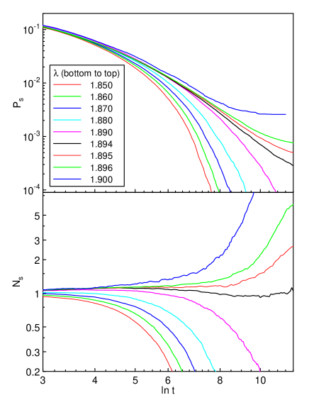
Figure 12: (Color online) $\ln P_{s}(t)$ and $\ln N_{s}(t)$ versus $\ln\ln t$ for the three-dimensional contact process on a diluted lattice ($p=0.3$, $L=400$, at least 5000 disorder realizations with 128 trials each).

A detailed quantitative analysis of the critical behavior requires significantly longer times and larger systems. It will be published elsewhere.

IV.3 Conclusions

Recently, a general classification of phase transitions in quenched disordered systems with short-range interactions has been suggested Vojta and Schmalian (2005); Vojta (2006). It is based on the effective dimensionality $d_{\rm eff}$ of the defects (or, equivalently, the rare regions.) Three cases can be distinguished.

(A) If $d_{\rm eff}$ is below the lower critical dimension $d_{c}^{-}$ of the problem, the rare region effects are exponentially weak, and the critical point is of conventional type. (B) In the second class, with $d_{\rm eff}=d_{c}^{-}$, the Griffiths effects are of strong power-law type and the critical behavior is controlled by an infinite-randomness fixed point with activated scaling. (C) For $d_{\rm eff}>d_{c}^{-}$, the rare regions can undergo the phase transition independently from the bulk system. This leads to a destruction of the sharp phase transition by smearing Vojta (2003).

The results of this paper agree with this general classification scheme as $d_{\rm eff}=d_{c}^{-}=0$ (this corresponds to rare regions being marginal with their life time depending exponentially on their size) leading to class B. In contrast, the contact process with extended (line or plane) defects falls into class C Vojta (2004); Dickison and Vojta (2005).

We conclude by pointing out that the unconventional behavior found in this paper may explain the striking absence of directed percolation scaling Hinrichsen (2000b) in at least some of the experiments. However, the extremely slow dynamics and narrow critical region will prove to be a challenge for the verification of the activated scaling scenario not just in simulations but also in experiments. We also emphasize that our results are of importance beyond absorbing state transitions. Since the strong-disorder renormalization group predicts our transition to be in the universality class of the two-dimensional random transverse-field Ising model, the critical behavior found here should be valid for this entire universality class.

References

- Zhdanov and Kasemo (1994) V. P. Zhdanov and B. Kasemo, Surface Science Reports 20, 111 (1994).
- Schmittmann and Zia (1995) B. Schmittmann and R. K. P. Zia, in Phase Transitions and Critical Phenomena, edited by C. Domb and J. L. Lebowitz (Academic, New York, 1995), vol. 17, p. 1.
- Marro and Dickman (1999) J. Marro and R. Dickman, Nonequilibrium Phase Transitions in Lattice Models (Cambridge University Press, Cambridge, 1999).
- Hinrichsen (2000a) H. Hinrichsen, Adv. Phys. 49, 815 (2000a).
- Odor (2004) G. Odor, Rev. Mod. Phys. 76, 663 (2004).
- Lübeck (2004) S. Lübeck, Int. J. Mod. Phys. B 31/32, 3977 (2004).
- Täuber et al. (2005) U. C. Täuber, M. Howard, and B. P. Vollmayr-Lee, J. Phys. A 38, R79 (2005).
- Grassberger and de la Torre (1979) P. Grassberger and A. de la Torre, Ann. Phys. (NY) 122, 373 (1979).
- Janssen (1981) H. K. Janssen, Z. Phys. B 42, 151 (1981).
- Grassberger (1982) P. Grassberger, Z. Phys. B 47, 365 (1982).
- Harris (1974a) T. E. Harris, Ann. Prob. 2, 969 (1974a).
- Ziff et al. (1986) R. M. Ziff, E. Gulari, and Y. Barshad, Phys. Rev. Lett. 56, 2553 (1986).
- Tang and Leschhorn (1992) L. H. Tang and H. Leschhorn, Phys. Rev. A 45, R8309 (1992).
- Pomeau (1986) Y. Pomeau, Physica D 23, 3 (1986).
- Hinrichsen (2000b) H. Hinrichsen, Braz. J. Phys. 30, 69 (2000b).
- Rupp et al. (2003) P. Rupp, R. Richter, and I. Rehberg, Phys. Rev. E 67, 036209 (2003).
- Takeuchi et al. (2007) K. A. Takeuchi, M. Kuroda, H. Chate, and M. Sano, Phys. Rev. Lett. 99, 234503 (2007).
- Harris (1974b) A. B. Harris, J. Phys. C 7, 1671 (1974b).
- Kinzel (1985) W. Kinzel, Z. Phys. B 58, 229 (1985).
- Noest (1986) A. J. Noest, Phys. Rev. Lett. 57, 90 (1986).
- Janssen (1997) H. K. Janssen, Phys. Rev. E 55, 6253 (1997).
- Bib (a) Some special versions of spatial disorder appear be lead to conventional behavior. A recent computational study of the contact process on a Voronoi triangulation (a random lattice with coordination disorder only) found critical behavior compatible with the clean DP universality class de Oliveira et al. (2008).
- Moreira and Dickman (1996) A. G. Moreira and R. Dickman, Phys. Rev. E 54, R3090 (1996).
- Dickman and Moreira (1998) R. Dickman and A. G. Moreira, Phys. Rev. E 57, 1263 (1998).
- Griffiths (1969) R. B. Griffiths, Phys. Rev. Lett. 23, 17 (1969).
- Noest (1988) A. J. Noest, Phys. Rev. B 38, 2715 (1988).
- Bramson et al. (1991) M. Bramson, R. Durrett, and R. H. Schonmann, Ann. Prob. 19, 960 (1991).
- Webman et al. (1998) I. Webman, D. B. Avraham, A. Cohen, and S. Havlin, Phil. Mag. B 77, 1401 (1998).
- Cafiero et al. (1998) R. Cafiero, A. Gabrielli, and M. A. Munoz, Phys. Rev. E 57, 5060 (1998).
- Hooyberghs et al. (2003) J. Hooyberghs, F. Igloi, and C. Vanderzande, Phys. Rev. Lett. 90, 100601 (2003).
- Hooyberghs et al. (2004) J. Hooyberghs, F. Igloi, and C. Vanderzande, Phys. Rev. E 69, 066140 (2004).
- Alcaraz et al. (1994) F. C. Alcaraz, M. Droz, M. Henkel, and V. Rittenberg, Ann. Phys. (NY) 230, 250 (1994).
- Ma et al. (1979) S. K. Ma, C. Dasgupta, and C. K. Hu, Phys. Rev. Lett. 43, 1434 (1979).
- Igloi and Monthus (2005) F. Igloi and C. Monthus, Phys. Rep. 412, 277 (2005).
- Fisher (1992) D. S. Fisher, Phys. Rev. Lett. 69, 534 (1992).
- Fisher (1995) D. S. Fisher, Phys. Rev. B 51, 6411 (1995).
- Vojta and Dickison (2005) T. Vojta and M. Dickison, Phys. Rev. E 72, 036126 (2005).
- Motrunich et al. (2000) O. Motrunich, S. C. Mau, D. A. Huse, and D. S. Fisher, Phys. Rev. B 61, 1160 (2000).
- Vojta (2006) T. Vojta, J. Phys. A 39, R143 (2006).
- Bib (b) We define is the fraction of sites removed rather than the fraction of sites present.
- Vojta and Lee (2006) T. Vojta and M. Y. Lee, Phys. Rev. Lett. 96, 035701 (2006).
- Dahmen et al. (2007) S. R. Dahmen, L. Sittler, and H. Hinrichsen, J. Stat. Mech. Theor Exp. p. P01011 (2007).
- Bib (c) At more general absorbing state transitions, e.g., with several absorbing states, the survival probability scales with an exponent which may be different from (see, e.g., Hinrichsen (2000a)).
- Bib (d) This relation relies on hyperscaling; it is only valid below the upper critical dimension , which is four for directed percolation.
- Dickison and Vojta (2005) M. Dickison and T. Vojta, J. Phys. A 38, 1199 (2005).
- Schonmann (1985) R. S. Schonmann, J. Stat. Phys. 41, 445 (1985).
- Dickman (1999) R. Dickman, Phys. Rev. E 60, R2441 (1999).
- Neugebauer et al. (2006) C. J. Neugebauer, S. V. Fallert, and S. N. Taraskin, Phys. Rev. E 74, 040101(R) (2006).
- Hoyos (2008) J. A. Hoyos, Phys. Rev. E 78, 032101 (2008).
- Chayes et al. (1986) J. T. Chayes, L. Chayes, D. S. Fisher, and T. Spencer, Phys. Rev. Lett. 57, 2999 (1986).
- Vojta and Schmalian (2005) T. Vojta and J. Schmalian, Phys. Rev. B 72, 045438 (2005).
- Vojta (2003) T. Vojta, Phys. Rev. Lett. 90, 107202 (2003).
- Vojta (2004) T. Vojta, Phys. Rev. E 70, 026108 (2004).
- de Oliveira et al. (2008) M. M. de Oliveira, S. G. Alves, S. C. Ferreira, and R. Dickman, Phys. Rev. E 78, 031133 (2008).