A modified characteristic finite element method for a fully nonlinear formulation of the semigeostrophic flow equations

Abstract

This paper develops a fully discrete modified characteristic finite element method for a coupled system consisting of the fully nonlinear Monge-Ampére equation and a transport equation. The system is the Eulerian formulation in the dual space for the B. J. Hoskins’ semigeostrophic flow equations, which are widely used in meteorology to model slowly varying flows constrained by rotation and stratification. To overcome the difficulty caused by the strong nonlinearity, we first formulate (at the differential level) a vanishing moment approximation of the semigeostrophic flow equations, a methodology recently proposed by the authors [17, 18], which involves approximating the fully nonlinear Monge-Ampére equation by a family of fourth order quasilinear equations. We then construct a fully discrete modified characteristic finite element method for the regularized problem. It is shown that under certain mesh and time stepping constraints, the proposed numerical method converges with an optimal order rate of convergence. In particular, the obtained error bounds show explicit dependence on the regularization parameter ${\varepsilon}$. Numerical tests are also presented to validate the theoretical results and to gauge the efficiency of the proposed fully discrete modified characteristic finite element method.

1 Introduction

The semigeostrophic flow equations, which were derived by B. J. Hoskins [22], is used in meteorology to model slowly varying flows constrained by rotation and stratification. They can be considered as an approximation of the Euler equations and are thought to be an efficient model to describe front formation (cf. [23, 10]). Under certain assumptions and in some appropriately chosen curve coordinates (called ‘dual space’, see Section 2), they can be formulated as the following coupled system consisting of the fully nonlinear Monge-Ampére equation and the transport equation:

(1) $$\det(D^{2}\psi^{*}) =\alpha\hskip 28.45274pt \text{in }\mathbb{R}^{3}\times(0,T],$$

(2) $$\frac{\partial\alpha}{\partial t}+{\mbox{\rm div\,}}(\mathbf{v}\alpha) =0\hskip 28.45274pt \text{in }\mathbb{R}^{3}\times(0,T],$$

(3) $$\alpha(x,0) =\alpha_{0}\hskip 28.45274pt \text{in }\mathbb{R}^{3}\times\{t=0\},$$

(4) $$\nabla\psi^{*} \subset\Omega,$$

and

(5) $$\mathbf{v}=(\nabla\psi^{*}-x)^{\bot}=(\psi^{*}_{x_{2}}-x_{2},x_{1}-\psi^{*}_{x_{1}},0).$$

Here, $\Omega\subset{\mathbb{R}}^{3}$ is a bounded domain, $\alpha$ is the density of a probability measure on $\mathbb{R}^{3}$, and $\psi^{*}$ denotes the Legendre transform of a convex function $\psi$. For any ${\mathbf{w}}=(w_{1},w_{2},w_{3})$, ${\mathbf{w}}^{\bot}:=(w_{2},-w_{1},0)$. We note that none of the variables $\alpha,\psi^{*}$, and ${\mathbf{v}}$ in the system is an original primitive variable appearing in the Euler equations. However, all primitive variables can be conveniently recovered from these non-physical variables (see Section 2 for the details).

In this paper, our goal is to numerically approximate the solution of (1)–(5). By inspecting the above system, one easily observes that there are three clear difficulties for achieving the goal. First, the equations are posed over an unbounded domain, which makes numerically solving the system infeasible. Second, the $\psi^{*}$-equation is the fully nonlinear Monge-Ampére equation. Numerically, little progress has been made in approximating second order fully nonlinear PDEs such as the Monge-Ampére equation. Third, equation (4) imposes a nonstandard constraint on the solution $\psi^{*}$, which often is called the second kind boundary condition for $\psi^{*}$ in the PDE community (cf. [3, 10]).

As a first step to approximate the solution of the above system, we must solve (1)–(3) over a finite domain, $U\subset\mathbb{R}^{3}$, which then calls for the use of artificial boundary condition techniques. For the second difficulty, we recall that a main obstacle is the fact that weak solutions (called viscosity solutions) for second order nonlinear PDEs are non-variational. This poses a daunting challenge for Galerkin type numerical methods such as finite element, spectral element, and discontinuous Galerkin methods, which are all based on variational formulations of PDEs. To overcome the above difficulty, recently we introduced a new approach in [17, 18, 19, 20, 25], called the vanishing moment method in order to approximate viscosity solutions of fully nonlinear second order PDEs. This approach gives rise a new notion of weak solutions, called moment solutions, for fully nonlinear second order PDEs. Furthermore, the vanishing moment method is constructive, so practical and convergent numerical methods can be developed based on the approach for computing viscosity solutions of fully nonlinear second order PDEs. The main idea of the vanishing moment method is to approximate a fully nonlinear second order PDE by a quasilinear higher order PDE. In this paper, we apply the methodology of the vanishing moment method, and approximate (1)–(3) by the following fourth order quasi-linear system:

(6) $$-\varepsilon\Delta^{2}\psi^{\varepsilon}+\det(D^{2}\psi^{\varepsilon}) =\alpha^{\varepsilon}\hskip 28.45274pt \text{in }U\times(0,T],$$

(7) $$\frac{\partial\alpha^{\varepsilon}}{\partial t}+{\mbox{\rm div\,}}(\mathbf{v}^{\varepsilon}\alpha^{\varepsilon}) =0\hskip 28.45274pt \text{in }U\times(0,T],$$

(8) $$\alpha^{\varepsilon}(x,0) =\alpha_{0}(x)\hskip 28.45274pt \text{in }{\mathbb{R}}^{3}\times\{t=0\},$$

where

(9) $${\mathbf{v}}^{\varepsilon}:=(\nabla\psi^{\varepsilon}-x)^{\bot}=(\psi^{\varepsilon}_{x_{2}}-x_{2},x_{1}-\psi^{\varepsilon}_{x_{1}},0).$$

It is easy to see that (6)–(9) is underdetermined, so extra constraints are required in order to ensure uniqueness. To this end, we impose the following boundary conditions and constraint to the above system:

(10) $$\frac{\partial\psi^{\varepsilon}}{\partial\nu} =0\hskip 28.45274pt \text{on }\partial U\times(0,T],$$

(11) $$\frac{\partial\Delta\psi^{\varepsilon}}{\partial\nu} =\varepsilon\hskip 28.45274pt \text{on }\partial U\times(0,T],$$

(12) $$\int_{U}\psi^{\varepsilon}dx =0\hskip 28.45274pt t\in(0,T],$$

where $\nu$ denotes the unit outward normal to $\partial U$. We remark that the choice of (11) intends to minimize the boundary layer due to the introduction of the singular perturbation term in (6) (see [17] for more discussions). Boundary condition (10) is used to minimize the “reflection” due to the introduction of the finite computational domain $U$. It can be regarded as a simple radiation boundary condition. An additional consequence of (10) is that it also effectively overcomes the third difficulty, which is caused by the nonstandard constraint (4), for solving system (1)–(5). Clearly, (12) is purely a mathematical technique for selecting a unique function from a class of functions differing from each other by an additive constant.

The specific goal of this paper is to formulate and analyze a modified characteristic finite element method for problem (6)–(12). The proposed method approximates the elliptic equation for $\psi^{\varepsilon}$ by conforming finite element methods (cf. [8]) and discretizes the transport equation for $\alpha^{\varepsilon}$ by a modified characteristic method due to Douglas and Russell [15]. We are particularly interested in obtaining error estimates that show explicit dependence on ${\varepsilon}$ for the proposed numerical method.

The remainder of this paper is organized as follows. In Section 2, we introduce the semigeostrophic flow equations and show how they can be formulated as the Monge-Ampére/transport system (1)–(5). In Section 3, we apply the methodology of the vanishing moment method to approximate (1)–(5) via (6)–(12), prove some properties of this approximation, and also state certain assumptions about this approximation. We then formulate our modified characteristic finite element method to numerically compute the solution of (6)–(12). Section 4 mirrors the analysis found in [20] where we analyze the numerical solution of the Monge-Ampére equation under small perturbations of the data. Section 4 is of independent interests in itself, but the main results will prove to be crucial in the next section. In Section 5, under certain mesh and time stepping constraints, we establish optimal order error estimates for the proposed modified characteristic finite element method. The main idea of the proof is to use the results of Section 4 and an inductive argument. Finally, in Section 6, we provide numerical tests to validate the theoretical results of the paper.

Standard space notation is adopted in this paper, we refer to [4, 21, 8] for their exact definitions. In particular, $(\cdot,\cdot)$ and $\langle\cdot,\cdot\rangle$ denote the $L^{2}$-inner products on $U$ and $\partial U$, respectively. $C$ is used to denote a generic positive constant which is independent of ${\varepsilon}$ and mesh parameters $h$ and $\Delta t$.

2 Derivation of the Monge-Ampére/transport formulation for the semigeostrophic flow equations

For the reader’s convenience and to provide necessary background, we shall first give a concise derivation of the Hoskins’ semigeostrophic flow equations [22] and then explain how the Hoskins’ model is reformulated as a coupled Monge-Ampére/transport system. Although our derivation essentially follows those of [22, 10, 3], we shall make an effort to streamline the ideas and key steps in a way which we thought should be more accessible to the numerical analysis community.

Let $\Omega\subset{\mathbb{R}}^{3}$ denote a bounded domain of the troposphere in the atmosphere. It is well known [24] that if fluids are assumed to be incompressible, their dynamics in such a domain $\Omega$ are governed by the following incompressible Boussinesq equations which are a version of the incompressible Euler equations:

(13) $$\frac{D{\mathbf{u}}}{Dt}+\nabla p =f{\mathbf{u}}^{\bot}-\frac{\theta}{\theta_{0}}g{\mathbf{e}}_{3} \qquad\text{in }\Omega\times(0,T],$$

(14) $$\frac{D\theta}{Dt} =0 \qquad\text{in }\Omega\times(0,T],$$

(15) $${\mbox{\rm div\,}}{\mathbf{u}} =0 \qquad\text{in }\Omega\times(0,T],$$

(16) $$\mathbf{u} =\mathbf{0} \qquad\text{on }\partial\Omega\times(0,T],$$

where ${\mathbf{e}}_{3}:=(0,0,1)$, $\mathbf{u}=(u_{1},u_{2},u_{3})$ is the velocity field, $p$ is the pressure, $\theta$ either denotes the temperature (in the case of atmosphere) or the density (in the case of ocean) of the fluid in question. $\theta_{0}$ is a reference value of $\theta$. Also

$$\frac{D}{Dt}:=\frac{\partial}{\partial t}+{\mathbf{u}}\cdot\nabla$$

denotes the material derivative. Recall that ${\mathbf{u}}^{\bot}:=(u_{2},-u_{1},0)$. Finally, $f$, assumed to be a positive constant, is known as the Coriolis parameter, and $g$ is the gravitational acceleration constant. We note that the term $f{\mathbf{u}}^{\bot}$ is the so-called Coriolis force which is an artifact of the earth’s rotation (cf. [30]).

Ignoring the (low order) material derivative term in (13) we get

(17) $$\nabla_{H}p =f{\mathbf{u}}^{\bot},$$

(18) $$\frac{\partial p}{\partial x_{3}} =-\frac{\theta}{\theta_{0}}g,$$

where

$$\nabla_{H}:=\Bigl{(}\frac{\partial}{\partial x_{1}},\frac{\partial}{\partial x_{2}},0\Bigr{)}.$$

Equation (17) is known as the geostrophic balance, which describes the balance between the pressure gradient force and the Coriolis force in the horizontal directions. Equation (18) is known as the hydrostatic balance in the literature, which describes the balance between the pressure gradient force and the gravitational force in the vertical direction. Define

(19) $${\mathbf{u}}_{g}:=f^{-1}(\nabla p)^{\bot}\qquad\mbox{and}\qquad{\mathbf{u}}_{ag}:={\mathbf{u}}-{\mathbf{u}}_{g},$$

which are often called the geostrophic wind and ageostrophic wind, respectively.

The geostrophic and hydrostatic balances give very simple relations between the pressure field and the velocity field. However, the dynamics of the fluids are missing in the description. To overcome this limitation, J. B. Hoskins [22] proposed so-called semigeostrophic approximation which is based on replacing the material derivative term $\frac{D{\mathbf{u}}}{Dt}$ by $\frac{D{\mathbf{u}}_{g}}{Dt}$ in (13). This then leads to the following semigeostrophic flow equations (in the primitive variables):

(20) $$\frac{D{\mathbf{u}}_{g}}{Dt}+(\nabla p)^{\bot} =f{\mathbf{u}}^{\bot} \qquad\text{in }\Omega\times(0,T],$$

(21) $$\frac{\partial p}{\partial x_{3}} =-\frac{\theta}{\theta_{0}}g \qquad\text{in }\Omega\times(0,T],$$

(22) $$\frac{D\theta}{Dt} =0 \qquad\text{in }\Omega\times(0,T],$$

(23) $${\mbox{\rm div\,}}{\mathbf{u}} =0 \qquad\text{in }\Omega\times(0,T],$$

(24) $${\mathbf{u}} =0 \qquad\text{on }\partial\Omega\times(0,T].$$

It is easy to see that after substituting ${\mathbf{u}}_{g}=f^{-1}(\nabla p)^{\bot}$, (20) is an evolution equation for $(\nabla p)^{\bot}$. There are no explicit dynamic equations for ${\mathbf{u}}$ in the above semigeostrophic flow model. Also, by the definition of the material derivative, $\frac{D{\mathbf{u}}_{g}}{Dt}=\frac{\partial{\mathbf{u}}_{g}}{\partial t}+({\mathbf{u}}\cdot\nabla){\mathbf{u}}_{g}$. We note that the full velocity ${\mathbf{u}}$ appears in the last term. Should ${\mathbf{u}}\cdot\nabla$ be replaced by ${\mathbf{u}}_{g}\cdot\nabla$ in the material derivative, the resulting model is known as the quasi-geostrophic flow equations (cf. [24]).

Due to the peculiar structure of the semigeostrophic flow equations, it is difficult to analyze and to numerically solve the equations. The first successful analytical approach is the one based on the fully nonlinear reformulation (1)–(5), which was first proposed in [5] and was further developed in [3, 23] (see [11] for a different approach). The main idea of the reformulation is to use time-dependent curved coordinates so the resulting system becomes partially decoupled. Apparently, the trade-off is the presence of stronger nonlinearity in the new formulation.

The derivation of the fully nonlinear reformulation (1)–(5) starts with introducing the so-called geopotential and geostrophic transformation

(25) $$\psi:=\frac{p}{f^{2}}+\frac{1}{2}|x_{H}|^{2},\qquad\Phi:=\nabla\psi;\qquad\mbox{where}\qquad x_{H}:=(x_{1},x_{2},0).$$

A direct calculation verifies that

$$\Phi:=x_{H}+\frac{1}{f^{2}}(\nabla p)^{\bot}-\frac{\theta}{\theta_{0}f^{2}}g{\mathbf{e}}_{3}=x_{H}+\frac{1}{f}{\mathbf{u}}_{g}-\frac{\theta}{\theta_{0}f^{2}}g{\mathbf{e}}_{3},$$

consequently, (20)–(22) can be rewritten compactly as

(26) $$\frac{D\Phi}{Dt}=fJ(\Phi-x),$$

where

$$J=\left(\begin{array}[]{rrr}0&-1&0\\ 1&0&0\\ 0&0&0\end{array}\right).$$

For any $x\in\Omega$, let $X(x,t)$ denote the fluid particle trajectory originating from $x$, i.e.,

$$\frac{dX(x,t)}{dt} ={\mathbf{u}}(X(x,t),t)\qquad\forall\,t>0,$$

$$X(x,0) =x.$$

Define the composite function

(27) $$\Psi(\cdot,t):=\Phi(\cdot,t)\circ X(\cdot,t)=\Phi(X(\cdot,t),t)=\nabla\psi(X(\cdot,t),t).$$

Then we have from (26)

(28) $$\frac{\partial\Psi(x,t)}{\partial t}=fJ(\Psi(x,t)-X(x,t))=f(\Psi(x,t)-X(x,t))^{\bot}.$$

Since the incompressibility assumption implies $X$ is volume preserving,

$$\det(\nabla X)=1,$$

which is equivalent to

(29) $$\int_{\Omega}g(X(x,t))dx=\int_{\Omega}g(x)dx\qquad\forall\,g\in C(\overline{\Omega}).$$

To summarize, we have reduced (20)–(23) into (27)–(29). It is easy to see that $\Psi(x,t)$ is not unique because one has a freedom in choosing the geopotential $\psi$. However, Cullen, Norbury, and Purser [12] (also see [10, 3, 23]) discovered the so-called Cullen-Norbury-Purser principle which says that $\Psi(x,t)$ must minimize the geostrophic energy at each time $t$. A consequence of this minimum energy principle is that the geopotential $\psi$ must be a convex function. Using the assumption that $\psi$ is convex and Brenier’s polar factorization theorem [5], Brenier and Benamou [3] proved existence of such a convex function $\psi$ and a measure preserving mapping $X$ which solves (27)–(29).

To relate (27)–(29) with (1), (2), and (4), let $\alpha(y,t)dy$ be the image measure of the Lebesgue measure $dx$ by $\Psi(x,t)$, that is

$$\int_{\Omega}g(\Psi(x,t))dx=\int_{\mathbb{R}^{3}}g(y)\alpha(y,t)dy\hskip 28.45274pt\forall g\in C_{c}(\mathbb{R}^{3}).$$

We note that the image measure $\alpha(y,t)dy$ is the push-forward $\Psi_{\#}dx$ of $dx$ by $\Psi(x,t)$, and $\alpha(y,t)$ is the density of $\Psi_{\#}dx$ with respect to the Lebesgue measure $dy$.

Assume that $\psi$ is sufficiently regular, it follows from (27) and (29) that

(30) $$\int_{\Omega}g(\Psi(x,t))dx=\int_{\Omega}g(\nabla\psi(X(x,t),t))dx=\int_{\Omega}g(\nabla\psi(x,t))dx\qquad\forall\,g\in C_{c}({\mathbb{R}}^{3}).$$

Using a change of variable $y=\nabla\psi(x,t)$ on the right and the definition of $\alpha(y,t)dy$ on the left we get

$$\int_{{\mathbb{R}}^{3}}g(y)\alpha(y,t)dy=\int_{{\mathbb{R}}^{3}}g(y)\det(D^{2}\psi^{*}(y,t))dy\qquad\forall\,g\in C_{c}({\mathbb{R}}^{3}),$$

where $\psi^{*}$ denotes the Legendre transform of $\psi$, that is,

(31) $$\psi^{*}(y,t)=\sup_{x\in\Omega}\bigl{(}x\cdot y-\psi(x,t)\bigr{)}.$$

Hence

$$\alpha(y,t)=\det(D^{2}\psi^{*}(y,t)),$$

which yields (1).

For convex function $\psi$, by a property of the Legendre transform we have $\nabla\psi^{*}(y,t)=x\in\Omega$. Hence $\nabla\psi^{*}\subset\Omega$, therefore, (4) holds.

Finally, for any $w\in C_{c}^{\infty}([-1,T];\mathbb{R}^{3})$, it follows from integration by parts and (28) that

$$-\int_{\Omega}w(\Psi(x,0),0)\,dx=\int_{0}^{T}\int_{\Omega}\frac{dw(\Psi(x,t),t)}{dt}\,dxdt$$

$$\qquad\qquad=\int_{0}^{T}\int_{\Omega}\Bigl{\{}\nabla w(\Psi(x,t),t)\cdot\frac{\partial\Psi(x,t)}{\partial t}+\frac{\partial w(\Psi(x,t),t)}{\partial t}\Bigr{\}}\,dxdt$$

$$\qquad\qquad=\int_{0}^{T}\int_{\Omega}\Bigl{\{}\nabla w(\Psi(x,t),t)\cdot f(\Psi(x,t)-X(x,t))^{\bot}+\frac{\partial w(\Psi(x,t),t)}{\partial t}\Bigr{\}}\,dxdt.$$

Making a change of variable $y=\nabla\psi(x,t)$ and using the definition of $\alpha(y,t)dy$ we get

(32) $$\int_{0}^{T}\int_{{\mathbb{R}}^{3}}\Bigl{\{}\frac{\partial w(y,t)}{\partial t}+f{\mathbf{v}}(y,t)\cdot\nabla w(y,t)\Bigr{\}}\alpha(y,t)\,dydt+\int_{{\mathbb{R}}^{3}}w(y,0)\alpha(y,0)\,dy=0,$$

where ${\mathbf{v}}$ is as in (5). Hence,

$$\frac{\partial\alpha(y,t)}{\partial t}+f{\mbox{\rm div\,}}({\mathbf{v}}(y,t)\alpha(y,t))=0,$$

which gives (3) as $f=1$ is assumed in Section 1.

We remark that (30) and (32) are weak formulations of (1) and (2), respectively. We also cite the following existence and regularity results for (1)-(3) and refer the reader to [3] for their proofs.

Theorem 2.1.

Let $\Omega_{0},\Omega\subset{\mathbb{R}}^{3}$ be two bounded Lipschitz domain. Suppose further that $\alpha_{0}\in L^{p}({\mathbb{R}}^{3})$ with $\alpha_{0}\geq 0$, $\text{supp}(\alpha_{0})\subset\Omega_{0}$, and $\int_{\Omega_{0}}\alpha_{0}(x)dx=|\Omega|$. Then for any $T>0$, $p>1$, (1)-(3) has a weak solution $(\psi^{*},\alpha)$ in the sense of (30) and (32). Furthermore, there exists an $R>0$ such that $\mbox{supp}(\alpha(x,t))\subset B_{R}(0)$ for all $t\in[0,T]$ and

$$\alpha\in L^{\infty}([0,T];L^{p}(B_{R}(0))) \quad\text{nonnegative},$$

$$\psi\in L^{\infty}([0,T];W^{1,\infty}(\Omega)) \quad\text{convex in physical space},$$

$$\psi^{*}\in L^{\infty}([0,T];W^{1,\infty}({\mathbb{R}}^{3}) \quad\text{convex in dual space}.$$

Remark 2.1.

(a). The above compact support result for $\alpha$ justifies our approach of solving the original infinite domain problem on a truncated computational domain $U$, in particular, if $U$ is chosen large enough so that $B_{R}(0)\subset U$.

(b). Since $\alpha$ and $\psi^{*}$ are not physical variables, one needs to recover the physical variables ${\mathbf{u}}$ and $p$ from $\alpha$ and $\psi^{*}$. This can be done by the following procedure. First, one constructs the geopotential $\psi$ from its Legendre transform $\psi^{*}$. Numerically, this can be done by fast inverse Legendre transform algorithms. Second, one recovers the pressure field $p$ from the geopotential $\psi$ using (25). Third, one obtains the geostrophic wind ${\mathbf{u}}_{g}$ and the full velocity field ${\mathbf{u}}$ from the pressure field $p$ using (19).

(c). Recently, Loeper [23] generalized the above results to the case where $\alpha$ is a global weak probability measure solution of the semigeostrophic equations.

(d). As a comparison, we recall that two-dimensional incompressible Euler equations (in the vorticity-stream function formulation) has the form

$$\Delta\phi =\omega \quad\mbox{in }\Omega\times(0,T],$$

$$\frac{\partial\omega}{\partial t}+{\mbox{\rm div\,}}({\mathbf{u}}\omega) =0 \quad\mbox{in }\Omega\times(0,T],$$

$${\mathbf{u}} =(\nabla\phi)^{\bot}.$$

Clearly, the main difference is that $\phi$-equation above is a linear equation while $\psi^{*}$ in (2) is a fully nonlinear equation.

We conclude this section by remarking that in the case that the gravity is omitted, then the flow becomes two-dimensional. Repeating the derivation of this section and dropping the third component of all vectors, we then obtained a $2$-d semigeostrophic flow model which has exactly the same form as (1)–(5) except that the definition of the operator $(\cdot)^{\perp}$ becomes ${\mathbf{w}}^{\perp}:=(w_{2},-w_{1})$ for ${\mathbf{w}}=(w_{1},w_{2})$, and ${\mathbf{v}}$ in (5) is replaced by

$${\mathbf{v}}=(\psi^{*}_{x_{2}}-x_{2},x_{1}-\psi^{*}_{x_{1}}).$$

Similarly, ${\mathbf{v}}^{\varepsilon}$ in (9) should be replaced by

$${\mathbf{v}}^{\varepsilon}=(\psi^{\varepsilon}_{x_{2}}-x_{2},x_{1}-\psi^{\varepsilon}_{x_{1}}).$$

In the remaining of this paper we shall consider numerical approximations of both $2$-d and $3$-d models.

3 Formulation of the numerical method

3.1 Formulation of the vanishing moment approximation

As pointed out in Section 1, the primary difficulty for analyzing and numerically approximating the semigeostrophic equations (1)–(5) is caused by the strong nonlinearity and non-uniqueness of the $\psi^{*}$-equation (i.e., Monge-Ampére equation. cf. [1, 21]). The strong nonlinearity makes the equation non-variational, so any Galerkin type numerical methods is not directly applicable to the fully nonlinear equation. Non-uniqueness is difficult to deal at the discrete level because no effective selection criterion is known in the literature which guarantees picking up the physical solution (i.e., the convex solution). Because of the above difficulties, very little progress was made in the past on developing numerical methods for the Monge-Ampére equation and other fully nonlinear second order PDEs (cf. [13, 28, 29]).

Very recently, we have developed a new approach, called the vanishing moment method, for solving the Monge-Ampére equation and other fully nonlinear second order PDEs (cf. [17, 18, 19, 20, 25, 26]). Our basic idea is to approximate a fully nonlinear second order PDE by a singularly perturbed quasilinear fourth order PDE. In the case of the Monge-Ampére equation, we approximate the fully nonlinear second order equation

(33) $$\det(D^{2}w)=\varphi$$

by the following fourth order quasilinear PDE

$$-\varepsilon\Delta^{2}w^{\varepsilon}+\det(D^{2}w^{\varepsilon})=\varphi\hskip 28.45274pt(\varepsilon>0)$$

accompanied by appropriate boundary conditions. Numerics of [18, 19, 20, 25] show that for fixed $\varphi\geq 0$, $w^{\varepsilon}$ converges to the unique convex solution $w$ of (33) as $\varepsilon\to 0^{+}$. Rigorous proof of the convergence in some special cases was carried out in [17]. Upon establishing the convergence of the vanishing moment method, one can use various well-established numerical methods (such as finite element, finite difference, spectral and discontinuous Galerkin methods) to solve the perturbed quasilinear fourth order PDE. Remarkably, our experiences so far suggest that the vanishing moment method always converges to the physical solution. The success motivates us to apply the vanishing moment methodology to the semigeostrophic model (1)–(5), which leads us to studying problem (6)–(12).

Remark 3.1.

Since a perturbation term is introduced in (6), it is also natural to introduce a “viscosity” term $-{\varepsilon}\Delta\alpha$ on the left-hand side of (7). We believe this should be another viable strategy and will further explore the idea and compare the anticipated new result with that of this paper.

Since (6)–(7) is a quasilinear system, we can define weak solutions for problem (6)–(12) in the usual way using integration by parts.

Definition 1.

A pair of functions $(\psi^{\varepsilon},\alpha^{\varepsilon})\in L^{\infty}((0,T);H^{2}(U))\times L^{2}((0,T);H^{1}(U))\cap H^{1}((0,T);L^{2}(U))$ is called a weak solution to (6)–(12) if they satisfy the following integral identities for almost every $t\in(0,T)$:

(34) $$-{\varepsilon}\bigl{(}\Delta\psi^{\varepsilon},\Delta v\bigr{)}+\bigl{(}\det(D^{2}\psi^{\varepsilon}),v\bigr{)} =(\alpha^{\varepsilon},v)+\langle{\varepsilon}^{2},v\rangle \qquad\forall v\in H^{2}(U),$$

(35) $$\Bigl{(}\frac{\partial\alpha^{\varepsilon}}{\partial t},w\Bigr{)}+\bigl{(}{\mathbf{v}}^{\varepsilon}\cdot\nabla\alpha^{\varepsilon},w\bigr{)} =0 \qquad\forall w\in H^{1}(U),$$

(36) $$\bigl{(}\alpha^{\varepsilon}(\cdot,0),\chi\bigr{)} =\bigl{(}\alpha_{0},\chi\bigr{)} \qquad\forall\chi\in L^{2}(U),$$

(37) $$(\psi^{\varepsilon},1) =0,$$

here ${\mathbf{v}}^{\varepsilon}=(\psi^{\varepsilon}_{x_{2}}-x_{2},x_{1}-\psi^{\varepsilon}_{x_{1}},0)$ when $d=3$ and ${\mathbf{v}}^{\varepsilon}=(\psi^{\varepsilon}_{x_{2}}-x_{2},x_{1}-\psi^{\varepsilon}_{x_{1}})$ when $d=2$, and we have used the fact that ${\mbox{\rm div\,}}{\mathbf{v}}^{\varepsilon}=0$.

For the continuation of the paper, we assume that there exists a unique solution to (6)–(12) such that $\psi^{\varepsilon}(x,t)$ is convex, $\alpha^{\varepsilon}(x,t)\geq 0$, and supp $\alpha^{\varepsilon}(x,t)\subset B_{R}(0)\subset U$ for all $t\in[0,T]$. We also assume $\psi^{\varepsilon}\in L^{2}((0,T);H^{s}(U))$ ($s\geq 3$), $\alpha^{\varepsilon}\in L^{2}((0,T);H^{p}(U))$ ($p\geq 2$), and that the following bounds hold (cf. [17]) for almost all $t\in[0,T]$

(38) $$\|\psi^{\varepsilon}(t)\|_{H^{j}}=O(\varepsilon^{\frac{1-j}{2}})\,\,(j=1,2,3),\qquad\|\Phi^{\varepsilon}(t)\|_{L^{\infty}}=O(\varepsilon^{-1}),$$

(39) $$\|\psi^{\varepsilon}(t)\|_{W^{j,\infty}}=O(\varepsilon^{1-j})\,\,(j=1,2),\qquad\|\alpha^{\varepsilon}(t)\|_{W^{1,\infty}}=O(\varepsilon^{-1}),$$

where $\Phi^{\varepsilon}=\text{cof}(D^{2}\psi^{\varepsilon})$ denotes the cofactor matrix of $D^{2}\psi^{\varepsilon}$.

As expected, the proof of the above assumptions is extensive and not easy. We do not intend to give a full proof in this paper. However, in the following we shall present a proof for a key assertion, that is, $\alpha^{\varepsilon}(x,t)\geq 0$ in $U\times[0,T]$ provided that $\alpha_{0}(x)\geq 0$ in ${\mathbb{R}}^{d}(\,d=2,3)$. Clearly, this assertion is important to ensure that $\psi^{\varepsilon}(\cdot,t)$ is a convex function for all $t\in[0,T]$.

Proposition 2.

Suppose $(\alpha^{\varepsilon},\psi^{\varepsilon})$ is a regular solution of (6)–(12). Assume $\alpha_{0}(x)\geq 0$ in ${\mathbb{R}}^{d}(\,d=2,3)$, then $\alpha^{\varepsilon}(x,t)\geq 0$ in $U\times[0,T]$.

Proof.

For any fixed $(x,t)\in U\times(0,T]$, let $X^{\varepsilon}(x,t;s)$ denote the characteristic curve passing through $(x,t)$ for the transport equation (7), that is.

$$\frac{dX^{\varepsilon}(x,t;s)}{ds} ={\mathbf{v}}^{\varepsilon}(X^{\varepsilon}(x,t;s),s)\qquad\quad\forall s\neq t,$$

$$X(x,t;t) =x.$$

Then the solution $\alpha^{\varepsilon}$ at $(x,t)$ can be written as

$$\alpha^{\varepsilon}(x,t)=\alpha_{0}(X^{\varepsilon}(x,t;0)).$$

Hence, $\alpha^{\varepsilon}(x,t)\geq 0$ for all $(x,t)\in U\times[0,T]$. The proof is complete. ∎

3.2 Formulation of modified characteristic finite element method

Let $\mathcal{T}_{h}$ be a quasiuniform triangulation or rectangular partition of $U$ with mesh size $h\in(0,1)$ and $V^{h}\subset H^{2}(U)$ denote a conforming finite element space (such as Argyris, Bell, Bogner–Fox–Schmit, and Hsieh–Clough–Tocher finite element spaces [8] when $d=2$) consisting of piecewise polynomial functions of degree $r\,(\geq 4)$ such that for any $v\in H^{s}(U)\ (s\geq 3)$

(40) $$\inf_{v_{h}\in V^{h}}\|v-v_{h}\|_{H^{j}}\leq h^{\ell-j}\|v\|_{H^{s}},\quad j=0,1,2;\,\ell=\min\{r+1,s\}.$$

Also let $W^{h}$ be a finite dimensional subspace of $H^{1}(U))$ consisting of piecewise polynomials of degree $k\,(\geq 1)$ associated with the mesh $\mathcal{T}_{h}$.

Set

(41) $$V^{h}_{0}:=\Bigl{\{}v_{h}\in V^{h};\ \frac{\partial v_{h}}{\partial\nu}\Bigl{|}_{\partial U}=0\Bigr{\}},\qquad V^{h}_{1}:=\{v_{h}\in V^{h}_{0};\,(v_{h},1)=0\},$$

(42) $$W^{h}_{0}:=\{w_{h}\in W^{h};\ w_{h}\big{|}_{\partial U}=0\},\qquad \tau:=\frac{(1,{\mathbf{v}}^{\varepsilon})}{\sqrt{1+|{\mathbf{v}}^{\varepsilon}|^{2}}}\in{\mathbb{R}}^{d+1}.$$

It is easy to check that

$$\frac{\partial}{\partial\tau}:=\tau\cdot\Bigl{(}\frac{\partial}{\partial t},\nabla\Bigr{)}=\frac{1}{\sqrt{1+|{\mathbf{v}}^{\varepsilon}|^{2}}}\Bigl{(}\frac{\partial}{\partial t}+{\mathbf{v}}^{\varepsilon}\cdot\nabla\Bigr{)}.$$

Hence, from (7) we have

(43) $$\frac{\partial\alpha^{\varepsilon}}{\partial\tau}=\frac{1}{\sqrt{1+|{\mathbf{v}}^{\varepsilon}|^{2}}}\Bigl{(}\frac{\partial\alpha^{\varepsilon}}{\partial t}+{\mathbf{v}}^{\varepsilon}\cdot\nabla\alpha^{\varepsilon}\Bigr{)}=0.$$

Here we have used the fact that ${\mbox{\rm div\,}}{\mathbf{v}}^{\varepsilon}=0$.

For a fixed positive integer $M$, let $\Delta t:=\frac{T}{M}$ and $t_{m}:=m\Delta t$ for $m=0,1,2,\cdots,M$. For any $x\in U$, let $\bar{x}:=x-{\mathbf{v}}^{\varepsilon}(x,t)\Delta t$. It follows from the Taylor’s formula that (cf. [14, 15])

(44) $$\frac{\partial\alpha^{\varepsilon}(x,t_{m})}{\partial\tau}=\frac{\alpha^{\varepsilon}(x,t_{m})-\alpha^{\varepsilon}(\bar{x},t_{m-1})}{\Delta t}+O(\Delta t)\qquad\mbox{for }m=1,2,\cdots,M.$$

Borrowing the ideas of [14, 15], we propose the following modified characteristic finite element method for problem (6)–(12):

Algorithm 1:

Step 1: Let $\alpha_{h}^{0}$ be the finite element interpolation or the elliptic projection of $\alpha_{0}$.

Step 2: For $m=0,1,2,\ldots M$, find $(\psi^{m}_{h},\alpha^{m+1}_{h})\in V_{1}^{h}\times W^{h}_{0}$ such that

(45) $$-\varepsilon(\Delta\psi_{h}^{m},\Delta v_{h})+(\det(D^{2}\psi_{h}^{m}),v_{h}) =(\alpha_{h}^{m},v_{h})+\langle\varepsilon^{2},v_{h}\rangle \qquad\forall v_{h}\in V^{h}_{0},$$

(46) $$(\psi_{h}^{m},1) =0,$$

(47) $$\bigl{(}\alpha_{h}^{m+1}-{\overline{\alpha}}_{h}^{m},w_{h}\bigr{)} =0 \qquad\forall w_{h}\in W^{h}_{0},$$

where

$${\overline{\alpha}}_{h}^{m}:=\alpha_{h}^{m}(\bar{x}_{h}),\qquad\bar{x}_{h}:=x-{\mathbf{v}}^{m}_{h}\Delta t,\qquad{\mathbf{v}}^{m}_{h}:=(\nabla\psi^{m}_{h}-x)^{\bot}.$$

In the case that $W^{h}$ is the continuous linear finite element space (i.e., $k=1$), we have the following lemma.

Lemma 3.

Let $k=1$ in the definition of $W^{h}$, suppose that $\alpha_{h}^{0}\geq 0$ in ${\mathbb{R}}^{d}(\,d=2,3)$, then the solution of Algorithm 1 satisfies $\alpha_{h}^{m}\geq 0$ in $U$ for all $m\geq 1$.

Proof.

In the case $k=1$, (47) immediately implies that

$$\alpha_{h}^{m+1}(P_{j})=\alpha_{h}^{m}(\overline{P}_{j}),$$

where $\{P_{j}\}$ denote the nodal points of the mesh ${\mathcal{T}}_{h}$ and $\overline{P}_{j}:=P_{j}-{\mathbf{v}}^{m}_{h}\Delta t$. Suppose that $\alpha_{h}^{m}(P_{j})\geq 0$ for all $j$. Since the basis functions of the linear element are nonnegative, then we have $\alpha_{h}^{m}(\overline{P}_{j})\geq 0$ for all $j$. Hence, $\alpha_{h}^{m+1}(P_{j})\geq 0$ for all $j$. Therefore, the assertion follows from the induction argument. ∎

Remark 3.2.

The positivity of $\alpha_{h}^{m}$ for all $m\geq 1$ gives hope to verify the convexity of $\psi_{h}^{m}$, which remains as an open problem (cf. [18, 19, 20]). For high order finite elements (i.e., $k\geq 2$), $\alpha_{h}^{m}$ might take negative values for some $m>0$ although we shall show later that the deviation from zero must be very small.

Let $(\psi^{\varepsilon},\alpha^{\varepsilon})$ be the solution of (6)–(12) and $(\psi^{m}_{h},\alpha^{m}_{h})$ be the solution of (45)-(47). In the subsequent sections we prove existence and uniqueness for $(\psi^{m}_{h},\alpha^{m}_{h})$ and provide optimal order error estimates for $\psi^{\varepsilon}(t_{m})-\psi^{m}_{h}$ and $\alpha^{\varepsilon}(t_{m})-\alpha^{m}_{h}$ under certain mesh and time stepping constraints. To this end, we first study (45) independently, which motivates us to analyze finite element approximations of the Monge-Ampére equation with small perturbations of the data. Such an analysis enables us to bound the error $\psi^{\varepsilon}(t_{m})-\psi^{m}_{h}$ in terms of of the error $\alpha^{\varepsilon}(t_{m})-\alpha^{m}_{h}$. We use similar techniques to those developed in [20] to carry out the analysis. With this result in hand, we use an inductive argument in Section 5 to get the desired error estimates for both $\psi^{\varepsilon}(t_{m})-\psi^{m}_{h}$ and $\alpha^{\varepsilon}(t_{m})-\alpha^{m}_{h}$.

4 Finite element approximations of the Monge-Ampére equation with small perturbations

As mentioned above, analyzing the error $\psi^{\varepsilon}(t_{m})-\psi^{m}_{h}$ motivates us to consider finite element approximations of the following auxiliary problem: for ${\varepsilon}>0$,

(48) $$-\varepsilon\Delta^{2}u^{\varphi}+\det(D^{2}u^{\varphi}) =\varphi\ (>0)\hskip 28.45274pt \text{in }U,$$

(49) $$\frac{\partial u^{\varphi}}{\partial\nu} =0\hskip 28.45274pt \text{on }\partial U,$$

(50) $$\frac{\partial\Delta u^{\varphi}}{\partial\nu} =\varepsilon\hskip 28.45274pt \text{on }\partial U,$$

(51) $$(u^{\varphi},1) =0,$$

whose weak formulation is defined as seeking $u^{\varphi}\in H^{2}(\Omega)$ such that

(52) $$-\varepsilon\bigl{(}\Delta u^{\varphi},\Delta v\bigr{)}+\bigl{(}\det(D^{2}u^{\varphi}),v\bigr{)} =\bigl{(}\varphi,v\bigr{)}+\langle\varepsilon^{2},v\rangle\qquad\forall v\in H^{2}(U),$$

(53) $$(u^{\varphi},1) =0.$$

We note that the finite element approximation of a similar Monge-Ampére problem was constructed and analyzed in [20], where the Dirichlet boundary condition was considered and the right-hand side function $\varphi$ is the same in the finite element scheme as in the PDE problem. In this section, we shall study the finite element approximation of (48)–(51) in which $\varphi$ is replaced by $\tilde{\varphi}:=\varphi+\delta\varphi$, where $\delta\varphi$ is some small perturbation of $\varphi$. Specifically, we analyze the following finite element approximation of (48)–(51): find $u^{\varphi}_{h}\in V^{h}_{1}$ such that

(54) $$-\varepsilon(\Delta u^{\varphi}_{h},\Delta v_{h})+(\det(D^{2}u^{\varphi}_{h}),v_{h}) =(\tilde{\varphi},v_{h})+\left\langle\varepsilon^{2},v_{h}\right\rangle\hskip 28.45274pt\forall v_{h}\in V^{h}_{0}.$$

As expected, we shall adapt the same ideas and techniques as those of [20] to analyze the above scheme. However, we shall omit some details if they are same as those of [20] but highlight the differences if they are significant, in particular, we shall trace how the error constants depend on ${\varepsilon}$ and $\delta\varphi$. Also, since the analysis in $2$-d and $3$-d are essentially the same, we shall only present the detailed analysis of the three dimensional case and make comments about the two dimensional case when there is a meaningful difference.

To analyze scheme (54), we first recall that (cf. [20]) the associated bilinear form of the linearization of the operator $M^{\varepsilon}(u^{\varphi}):=-\varepsilon\Delta^{2}u^{\varphi}+\det(D^{2}u^{\varphi})$ at the solution $u^{\varphi}$ is given by

(55) $$B[v,w]:=\varepsilon(\Delta v,\Delta w)+(\Phi^{\varphi}\nabla v,\nabla w),$$

where $\Phi^{\varphi}={\rm cof}(D^{2}u^{\varphi})$ denotes the cofactor matrix of $D^{2}u^{\varphi}$.

Next, we define a linear operator $T^{\varphi}:V^{h}_{1}\to V^{h}_{1}$ such that for $w_{h}\in V^{h}_{1}$, $T^{\varphi}(w_{h})\in V^{h}_{1}$ is the solution of following problem:

(56) $$B[w_{h}-T^{\varphi}(w_{h}),v_{h}]=\varepsilon(\Delta w_{h},\Delta v_{h}) -(\det(D^{2}w_{h}),v_{h})$$

$$+(\tilde{\varphi},v_{h})+\langle\varepsilon^{2},v_{h}\rangle\quad\forall v_{h}\in V^{h}_{0}.$$

It follows from [20, Theorem 3.5] that $T^{\varphi}$ is well-defined. Also, it is easy to see that any fixed point of $T^{\varphi}$ is a solution to (54). We now show that if $\|\delta\varphi\|_{L^{2}}$ is sufficiently small, then indeed, $T^{\varphi}$ has a unique fixed point in a neighborhood of $u^{\varphi}$. To this end, we set

$$\mathbb{B}_{h}(\rho):=\bigl{\{}v_{h}\in V^{h}_{1};\ \|v_{h}-I_{h}u^{\varphi}\|_{H^{2}}\leq\rho\bigr{\}},$$

where $I_{h}u^{\varphi}$ denotes the finite element interpolant of $u^{\varphi}$ onto $V^{h}_{1}$.

Before we continue, we state a lemma concerning the divergence row property of cofactor matrices. A short proof can be found in [16].

Lemma 4.1.

Given a vector-valued function $\mathbf{w}=(w_{1},w_{2},\cdots,w_{n}):U\rightarrow\mathbb{R}^{n}$. Assume $\mathbf{w}\in[C^{2}(U)]^{n}$. Then the cofactor matrix $\text{\rm cof}(D\mathbf{w})$ of the gradient matrix $D\mathbf{w}$ of $\mathbf{w}$ satisfies the following row divergence-free property:

(57) $${\mbox{\rm div\,}}(\text{\rm cof}(D\mathbf{w}))_{i}=\sum_{j=1}^{n}\partial_{x_{j}}(\text{\rm cof}(D\mathbf{w}))_{ij}=0\qquad\text{\rm for }i=1,2,\cdots,n,$$

where $(\text{\rm cof}(D\mathbf{w}))_{i}$ and $(\text{\rm cof}(D\mathbf{w}))_{ij}$ denote respectively the $i$th row and the $(i,j)$-entry of $\text{\rm cof}(D\mathbf{w})$.

Throughout the rest of this section, we assume $u^{\varphi}\in H^{s}$, set $\ell={\rm min}\{r+1,s\}$, and assume the following bounds (compare to those of [20] and (38)): for $j=1,2,3,$

(58) $$\|u^{\varphi}\|_{H^{j}}=O(\varepsilon^{\frac{1-j}{2}}),\quad\|u^{\varphi}\|_{W^{2,\infty}}=O(\varepsilon^{-1}),\quad\|\Phi^{\varphi}\|_{L^{\infty}}=O(\varepsilon^{-1}).$$

We then have the following results.

Lemma 4.2.

There exists a constant $C_{1}(\varepsilon)=O(\varepsilon^{-1})$ such that

(59) $$\|I_{h}u^{\varphi}-T^{\varphi}(I_{h}u^{\varphi})\|_{H^{2}}\leq C_{1}(\varepsilon)\bigl{(}\varepsilon^{-2}h^{\ell-2}\|u^{\varphi}\|_{H^{\ell}}+\|\delta\varphi\|_{H^{-2}}\bigr{)}.$$

Proof.

To ease notation set $s_{h}=I_{h}u^{\varphi}-T^{\varphi}(I_{h}u^{\varphi})$ and $\eta=I_{h}u^{\varphi}-u^{\varphi}$. Then for any $v_{h}\in V^{h}_{0}$, we use the Mean Value Theorem to get

$$B[s_{h},v_{h}] =\varepsilon(\Delta(I_{h}u^{\varphi},\Delta v_{h})-(\det(D^{2}(I_{h}u^{\varphi}),v_{h})$$

$$\hskip 28.90755pt+(\tilde{\varphi},v_{h})+\langle\varepsilon^{2},v_{h}\rangle$$

$$=\varepsilon(\Delta\eta,\Delta v_{h})+(\det(D^{2}u^{\varphi})-\det(D^{2}(I_{h}u^{\varphi}),v_{h})+(\delta\varphi,v_{h})$$

$$=\varepsilon(\Delta\eta,\Delta v_{h})+(\Upsilon^{\varepsilon}:D^{2}(u^{\varphi}-I_{h}u^{\varphi}),v_{h})+(\delta\varphi,v_{h}),$$

where $\Upsilon^{\varepsilon}={\rm cof}(\tau D^{2}(I_{h}u^{\varphi})+(1-\tau)D^{2}u^{\varphi})$ for $\tau\in[0,1]$.

On noting that

$$|\Upsilon_{ij}|=|\text{cof}(\tau D^{2}(I_{h}u^{\varphi})+(1-\tau)D^{2}u^{\varphi})_{ij}|=\bigl{|}\det\bigl{(}\tau D^{2}(I_{h}u^{\varphi})\big{|}_{ij}+(1-\tau)D^{2}u^{\varphi}\big{|}_{ij}\bigr{)}\bigr{|},$$

where $D^{2}u^{\varphi}\big{|}_{ij}$ denotes the resulting $2\times 2$ matrix after deleting the $i^{th}$ row and $j^{th}$ column of $D^{2}u^{\varphi}$, we obtain

$$|(\Psi^{\varepsilon})_{ij}| \leq 2\max_{k\neq i,\ell\neq j}\left(|\tau(D^{2}(I_{h}u^{\varphi})_{k\ell}+(1-\tau)(D^{2}u^{\varphi})_{k\ell}|\right)^{2}$$

$$\leq C\max_{k\neq i,\ell\neq j}|(D^{2}u^{\varphi})_{k\ell}|^{2}\leq C\|D^{2}u^{\varphi}\|_{L^{\infty}}^{2}.$$

Hence, from (58) it follows that $\|\Upsilon^{\varepsilon}\|_{L^{\infty}}=O(\varepsilon^{-2})$. Thus,

$$B[s_{h},v_{h}] \leq\varepsilon\|\Delta\eta\|_{L^{2}}\|\Delta v_{h}\|_{L^{2}}+C\varepsilon^{-2}\|D^{2}\eta\|_{L^{2}}\|v_{h}\|_{L^{2}}+\|\delta\varphi\|_{H^{-2}}\|v_{h}\|_{H^{2}}$$

$$\leq C\bigl{(}\varepsilon^{-2}\|\eta\|_{H^{2}}+\|\delta\varphi\|_{H^{-2}}\bigr{)}\|v_{h}\|_{H^{2}}.$$

Finally, using the coercivity of $B[\cdot,\cdot]$ we get

$$\|s_{h}\|_{H^{2}} \leq C_{1}(\varepsilon)\bigl{(}\varepsilon^{-2}h^{\ell-2}\|u^{\varphi}\|_{H^{\ell}}+\|\delta\varphi\|_{H^{-2}}\bigr{)}.$$

The proof is complete. ∎

Lemma 4.3.

There exists $h_{0}>0$ such that for $h\leq h_{0}$, there exists an $\rho=\rho(h,\varepsilon)$ such that for any $v_{h},w_{h}\in\mathbb{B}_{h}(\rho)$ there holds

(60) $$\|T^{\varphi}(v_{h})-T^{\varphi}(w_{h})\|_{H^{2}}\leq\frac{1}{2}\|v_{h}-w_{h}\|_{H^{2}}.$$

Proof.

From the definitions of $T^{\varphi}(v_{h})$ and $T^{\varphi}(w_{h})$ we get for any $z_{h}\in V^{h}_{0}$

$$B[T^{\varphi}(v_{h}) -T^{\varphi}(w_{h}),z_{h}]$$

$$=\left(\Phi^{\varphi}(\nabla v_{h}-\nabla w_{h}),\nabla z_{h}\right)+\left(\text{det}(D^{2}v_{h})-\text{det}(D^{2}w_{h}),z_{h}\right).$$

Adding and subtracting $\det(D^{2}v_{h}^{\mu})$ and $\det(D^{2}w_{h}^{\mu})$, where $v_{h}^{\mu}$ and $w_{h}^{\mu}$ denote the standard mollifications of $v_{h}$ and $w_{h}$, respectively, yields

$$B[T^{\varphi}(v_{h})-T^{\varphi}(w_{h}),z_{h}]$$

$$\quad=(\Phi^{\varphi}(t_{m})(\nabla v_{h}-\nabla w_{h}),\nabla z_{h})+(\text{det}(D^{2}v^{\mu}_{h})-\text{det}(D^{2}w^{\mu}_{h}),z_{h})$$

$$\hskip 49.79231pt+(\text{det}(D^{2}v_{h})-\text{det}(D^{2}v_{h}^{\mu}),z_{h})+(\text{det}(D^{2}w^{\mu}_{h})-\text{det}(D^{2}w_{h}),z_{h})$$

$$\quad=(\Phi^{\varphi}(\nabla v_{h}-\nabla w_{h}),\nabla z_{h})+(\Psi_{h}:(D^{2}v^{\mu}_{h}-D^{2}w^{\mu}_{h}),z_{h})$$

$$\hskip 49.79231pt+(\text{det}(D^{2}v_{h})-\text{det}(D^{2}v_{h}^{\mu}),z_{h})+(\text{det}(D^{2}w^{\mu}_{h})-\text{det}(D^{2}w_{h}),z_{h}),$$

where $\Psi_{h}=\text{cof}(D^{2}v_{h}^{\mu}+\tau(D^{2}w_{h}^{\mu}-D^{2}v_{h}^{\mu}))$ for $\tau\in[0,1]$.

Using Lemma 4.1 and Sobolev’s inequality we have

(61) $$B[T^{\varphi}(v_{h})-T^{\varphi}(w_{h}),z_{h}]$$

$$\qquad=((\Phi^{\varphi}-\Psi_{h})(\nabla v_{h}-\nabla w_{h}),\nabla z_{h})+(\Psi_{h}(\nabla v_{h}-\nabla v_{h}^{\mu}),\nabla z_{h})$$

$$\qquad\qquad+(\Psi_{h}(\nabla w_{h}^{\mu}-\nabla w_{h}),z_{h})+(\text{det}(D^{2}v_{h})-\text{det}(D^{2}v_{h}^{\mu}),z_{h})$$

$$\qquad\qquad+(\text{det}(D^{2}w^{\mu}_{h})-\text{det}(D^{2}w_{h}),z_{h})$$

$$\qquad\leq C\Bigl{\{}\|\Phi^{\varphi}-\Psi_{h}\|_{L^{2}}\|v_{h}-w_{h}\|_{H^{2}}+\|\Psi_{h}\|_{L^{2}}\bigl{[}\|v_{h}-v_{h}^{\mu}\|_{H^{2}}$$

$$\qquad\qquad+\|w_{h}-w_{h}^{\mu}\|_{H^{2}}\bigr{]}+\|\text{det}(D^{2}v_{h})-\text{det}(D^{2}v_{h}^{\mu})\|_{L^{2}}$$

$$\qquad\qquad+\|\text{det}(D^{2}w_{h})-\text{det}(D^{2}w_{h}^{\mu})\|_{L^{2}}\Bigr{\}}\|z_{h}\|_{H^{2}}.$$

It follows from the Mean Value Theorem that

$$\|(\Phi^{\varphi}-\Psi_{h})_{ij}\|_{L^{2}} =\|\det(D^{2}u^{\varphi}\big{|}_{ij})-\det(D^{2}v_{h}^{\mu}\big{|}_{ij}+\tau(D^{2}w_{h}^{\mu}\big{|}_{ij}-D^{2}v_{h}^{\mu}\big{|}_{ij}))\|_{L^{2}}$$

$$=\|\Lambda^{ij}:(D^{2}u^{\varphi}\big{|}_{ij}-(D^{2}v_{h}^{\mu}\big{|}_{ij}+\tau(D^{2}w_{h}^{\mu}\big{|}_{ij}-D^{2}v_{h}^{\mu}\big{|}_{ij})))\|_{L^{2}},$$

where $\Lambda^{ij}=\text{cof}(D^{2}u^{\varphi}\big{|}_{ij}+\lambda(D^{2}v_{h}^{\mu}\big{|}_{ij}+\tau(D^{2}w_{h}^{\mu}\big{|}_{ij}-D^{2}v_{h}^{\mu}\big{|}_{ij})))\in\mathbf{R}^{2\times 2}$ for $\lambda\in[0,1]$.

We bound $\|\Lambda^{ij}\|_{L^{\infty}}$ as follows:

$$\|\Lambda^{ij}\|_{L^{\infty}} =\|\text{cof}(D^{2}u^{\varphi}\big{|}_{ij}+\lambda(D^{2}v_{h}^{\mu}\big{|}_{ij}+\tau(D^{2}w_{h}^{\mu}\big{|}_{ij}-D^{2}v_{h}^{\mu}\big{|}_{ij})))\|_{L^{\infty}}$$

$$=\|D^{2}u^{\varphi}\big{|}_{ij}+\lambda(D^{2}v_{h}^{\mu}\big{|}_{ij}+\tau(D^{2}w_{h}^{\mu}\big{|}_{ij}-D^{2}v_{h}^{\mu}\big{|}_{ij}))\|_{L^{\infty}}$$

$$\leq C\bigl{(}\varepsilon^{-1}+h^{-\frac{3}{2}}\rho+\|D^{2}v_{h}^{\mu}-D^{2}v_{h})\|_{L^{\infty}}+\|D^{2}w_{h}^{\mu}-D^{2}w_{h}\|_{L^{\infty}}\bigr{)},$$

where we used the triangle inequality followed by the inverse inequality and (58). Combining the above two inequalities we get

$$\|(\Phi^{\varphi}-\Psi_{h})_{ij}\|_{L^{2}} \leq\|\Lambda^{ij}\|_{L^{\infty}}\|D^{2}u^{\varphi}\big{|}_{ij}-(D^{2}v_{h}^{\mu}\big{|}_{ij}+\tau(D^{2}w_{h}^{\mu}\big{|}_{ij}-D^{2}v_{h}^{\mu}\big{|}_{ij}))\|_{L^{2}}$$

$$\leq C\bigl{(}\varepsilon^{-1}+h^{-\frac{3}{2}}\rho+\|D^{2}v_{h}^{\mu}-D^{2}v_{h}\|_{L^{\infty}}+\|D^{2}w_{h}^{\mu}-D^{2}w_{h}\|_{L^{\infty}}\bigr{)}$$

$$\quad\times\bigl{(}h^{\ell-2}\|u^{\varphi}\|_{H^{\ell}}+\rho+\|D^{2}v_{h}-D^{2}v_{h}^{\mu}\|_{L^{2}}+\|D^{2}w_{h}^{\mu}-D^{2}w_{h}\|_{L^{2}}\bigr{)}.$$

Hence,

(62) $$\|\Phi^{\varphi}-\Psi_{h}\|_{L^{2}} \leq C\bigl{(}\varepsilon^{-1}+h^{-\frac{3}{2}}\rho+\|D^{2}v_{h}^{\mu}-D^{2}v_{h}\|_{L^{\infty}}+\|D^{2}w_{h}^{\mu}-D^{2}w_{h}\|_{L^{\infty}}\bigr{)}$$

$$\quad\times\bigl{(}h^{\ell-2}\|u^{\varphi}\|_{H^{\ell}}+\rho+\|D^{2}v_{h}-D^{2}v_{h}^{\mu}\|_{L^{2}}+\|D^{2}w_{h}^{\mu}-D^{2}w_{h}\|_{L^{2}}\bigr{)}.$$

Applying (62) to (61) and setting $\mu\to 0$ yield

$$B[T^{\varphi}(v_{h})-T^{\varphi}(w_{h}),z_{h}]\leq C\bigl{(}\varepsilon^{-1}+h^{-\frac{3}{2}}\rho\bigr{)}\bigl{(}h^{\ell-2}\|u^{\varphi}\|_{H^{\ell}}+\rho\bigr{)}\|v_{h}-w_{h}\|_{H^{2}}\|z_{h}\|_{H^{2}}.$$

Using the coercivity of $B[\cdot,\cdot]$ we get

(63) $$\|T^{\varphi}(v_{h})-T^{\varphi}(w_{h})\|_{H^{2}}\leq C\varepsilon^{-1}\bigl{(}\varepsilon^{-1}+h^{-\frac{3}{2}}\rho\bigr{)}\bigl{(}h^{\ell-2}\|u^{\varphi}\|_{H^{\ell}}+\rho\bigr{)}\|v_{h}-w_{h}\|_{H^{2}}.$$

Finally, setting $h_{0}=O\left(\frac{\varepsilon^{2}}{\|u^{\varphi}\|_{H^{\ell}}}\right)^{\frac{1}{\ell-2}}$, $h\leq h_{0}$, and $\rho=O({\rm min}\{\varepsilon^{2},\varepsilon h^{\frac{3}{2}}\})$, it then follows from (63) that

$$\|T^{\varphi}(v_{h})-T^{\varphi}(w_{h})\|_{H^{2}}\leq\frac{1}{2}\|v_{h}-w_{h}\|_{H^{2}}\hskip 28.45274pt\forall v_{h},w_{h}\in\mathbb{B}_{h}(\rho).$$

The proof is complete ∎

With the help of the above two lemmas, we are ready to state and prove our main results of this section.

Theorem 4.1.

Suppose $\|\delta\varphi\|_{H^{-2}}=O({\rm min}\{\varepsilon^{3},\varepsilon^{2}h^{\frac{3}{2}}\})$. Then there exists an $h_{1}>0$ such that for $h\leq h_{1}$, there exists a unique solution $u^{\varphi}_{h}\in V^{h}_{1}$ solving (54). Furthermore, there holds the following error estimate:

(64) $$\|u^{\varphi}-u^{\varphi}_{h}\|_{H^{2}}\leq C_{2}(\varepsilon)\bigl{(}\varepsilon^{-2}h^{\ell-2}\|u^{\varphi}\|_{H^{\ell}}+\|\delta\varphi\|_{H^{-2}}\bigr{)}$$

with $C_{2}(\varepsilon)=O(\varepsilon^{-1})$.

Proof.

To show the first claim, we set

$$h_{1}=O\left({\rm min}\left\{\left(\frac{\varepsilon^{4}}{\|u^{\varphi}\|_{H^{\ell}}}\right)^{\frac{2}{2\ell-7}},\left(\frac{\varepsilon^{5}}{\|u^{\varphi}\|_{H^{\ell}}}\right)^{\frac{1}{\ell-2}}\right\}\right).$$

Fix $h\leq h_{1}$ and set $\rho_{1}=2C_{1}(\varepsilon)\bigl{(}\varepsilon^{-2}h^{\ell-2}\|u^{\varphi}\|_{H^{\ell}}+\|\delta\varphi\|_{H^{-2}}\bigr{)}$. Then we have $\rho_{1}\leq C{\rm min}\{\varepsilon^{2},\varepsilon h^{\frac{3}{2}}\}$.

Next, let $v_{h}\in\mathbb{B}_{h}(\rho_{1})$. Using the triangle inequality and Lemmas 4.2 and 4.3 we get

$$\|I_{h}u^{\varphi}-T^{\varphi}(v_{h})\|_{H^{2}} \leq\|I_{h}u^{\varphi}-T^{\varphi}(I_{h}u^{\varphi})\|_{H^{2}}+\|T^{\varphi}(I_{h}u^{\varphi})-T^{\varphi}(v_{h})\|_{H^{2}}$$

$$\leq C_{1}(\varepsilon)\bigl{(}\varepsilon^{-2}h^{\ell-2}\|u^{\varphi}\|_{H^{\ell}}+\|\delta\varphi\|_{H^{-2}}\bigr{)}+\frac{1}{2}\|I_{h}u^{\varphi}-v_{h}\|_{H^{2}}$$

$$\leq\frac{\rho_{1}}{2}+\frac{\rho_{1}}{2}=\rho_{1}.$$

Hence, $T^{\varphi}(v_{h})\in\mathbb{B}_{h}(\rho_{1})$. In addition, by (60) we know that $T^{\varphi}$ is a contracting mapping in $\mathbb{B}_{h}(\rho_{1})$. Thus, the Brouwer’s Fixed Point Theorem [21] guarantees that there exists a unique fixed point $u^{\varphi}_{h}\in\mathbb{B}_{h}(\rho_{1})$ which is a solution to (54).

Finally, using the triangle inequality we get

$$\|u^{\varphi}-u^{\varphi}_{h}\|_{H^{2}} \leq\|u^{\varphi}-I_{h}u^{\varphi}\|_{H^{2}}+\|I_{h}u^{\varphi}-u^{\varphi}_{h}\|_{H^{2}}\leq Ch^{\ell-2}\|u^{\varphi}\|_{H^{\ell}}+\rho_{1}$$

$$\leq C_{2}(\varepsilon)\bigl{(}\varepsilon^{-2}h^{\ell-2}\|u^{\varphi}\|_{H^{\ell}}+\|\delta\varphi\|_{H^{-2}}\bigr{)}.$$

∎

Theorem 4.2.

In addition to the hypothesis of Theorem 4.1, assume that the linearization of $M^{\varepsilon}$ at $u^{\varphi}$ (see (55)) is $H^{3}$-regular with the regularity constant $C_{s}(\varepsilon)$. Furthermore, assume that $\|\delta\varphi\|_{H^{-2}}=O(C^{-1}_{s}(\varepsilon)\varepsilon^{2})$. Then there exists an $h_{2}>0$ such that for $h\leq h_{2}$, there holds

(65) $$\|u^{\varphi}-u^{\varphi}_{h}\|_{H^{1}} \leq C_{s}(\varepsilon)\Bigl{\{}C_{3}(\varepsilon)h^{\ell-1}\|u^{\varphi}\|_{H^{\ell}}+(C_{4}(\varepsilon)h+1)\|\delta\varphi\|_{H^{-2}}\Bigr{\}},$$

where $C_{3}(\varepsilon)=C_{2}(\varepsilon)\varepsilon^{-\frac{5}{2}}$ and $C_{4}(\varepsilon)=C_{2}(\varepsilon)\varepsilon^{-\frac{1}{2}}.$

Proof.

Let $e^{\varphi}:=u^{\varphi}-u_{h}^{\varphi}$ and $u^{\varphi,\mu}_{h}$ denote a standard mollification of $u_{h}^{\varphi}$. We note that $e^{\varphi}$ satisfies the following error equation:

(66) $$\varepsilon(\Delta e^{\varphi},\Delta z_{h})+(\text{det}(D^{2}u_{h}^{\varphi})-\text{det}(D^{2}u^{\varphi}),z_{h})+(\delta\varphi,z_{h})=0\hskip 28.45274pt\forall z_{h}\in V^{h}_{0}.$$

Using (66), the Mean Value Theorem, and Lemma 4.1 we have

(67) $$0=\varepsilon(\Delta e^{\varphi},\Delta z_{h}) -(\tilde{\Phi}\nabla(u^{\varphi,\mu}_{h}-u^{\varphi}),\nabla z_{h})+(\delta\varphi,z_{h})$$

$$+(\text{det}(D^{2}u^{\varphi}_{h})-\text{det}(D^{2}u^{\varphi,\mu}_{h}),z_{h}),$$

where $\tilde{\Phi}=\text{cof}(D^{2}u^{\varphi,\mu}_{h}+\tau(D^{2}u^{\varphi}-D^{2}u^{\varphi,\mu}_{h}))$ for $\tau\in[0,1]$.

Next, let $\phi\in V_{0}\cap H^{3}$ be the unique solution to the following problem:

$$B[\phi,z]=(\nabla e^{\varphi},\nabla z)\hskip 28.45274pt\forall z\in V_{0}.$$

The regularity assumption implies that

(68) $$\|\phi\|_{H^{3}}\leq C_{s}(\varepsilon)\|\nabla e^{\varphi}\|_{L^{2}}.$$

We then have

$$\|\nabla e^{\varphi}\|_{L^{2}}^{2} =\varepsilon(\Delta e^{\varphi},\Delta\phi)+(\Phi^{\varphi}\nabla\phi,\nabla e_{h}^{\varphi})$$

$$=\varepsilon(\Delta e^{\varphi},\Delta(\phi-I_{h}\phi))+(\Phi^{\varphi}\nabla e^{\varphi}_{h},\nabla(\phi-I_{h}\phi))+\varepsilon(\Delta e^{\varphi},\Delta(I_{h}\phi))$$

$$\quad+(\Phi^{\varphi}\nabla e^{\varphi},\nabla(I_{h}\phi))-\varepsilon(\Delta e^{\varphi},\Delta(I_{h}\phi))-(\tilde{\Phi}\nabla(u^{\varphi}-u^{\varphi,\mu}_{h}),\nabla(I_{h}\phi))$$

$$\quad-(\text{det}(D^{2}u^{\varphi}_{h})-\text{det}(D^{2}u^{\varphi,\mu}_{h}),I_{h}\phi)-(\delta\varphi,I_{h}\phi)$$

(69) $$=\varepsilon(\Delta e_{h}^{\varphi},\Delta(\phi-I_{h}\phi))+(\Phi^{\varphi}\nabla e^{\varphi},\nabla(\phi-I_{h}\phi))$$

$$\quad+((\Phi^{\varphi}-\tilde{\Phi})\nabla e^{\varphi},\nabla(I_{h}\phi))+(\tilde{\Phi}\nabla(u^{\varphi,\mu}_{h}-u^{\varphi}_{h}),\nabla(I_{h}\phi))$$

$$\quad+(\text{det}(D^{2}u^{\varphi,\mu}_{h})-\text{det}(D^{2}u^{\varphi}_{h}),I_{h}\phi)-(\delta\varphi,I_{h}\phi)$$

$$\leq\varepsilon\|\Delta e^{\varphi}\|_{L^{2}}\|\Delta(\phi-I_{h}\phi)\|_{L^{2}}+C\|\Phi^{\varphi}\|_{L^{2}}\|e^{\varphi}\|_{H^{2}}\|\phi-I_{h}\phi\|_{H^{2}}$$

$$\quad+C\|\Phi^{\varphi}-\tilde{\Phi}\|_{L^{2}}\|\nabla e^{\varphi}\|_{L^{2}}\|\nabla(I_{h}\phi)\|_{L^{\infty}}+C\|\tilde{\Phi}\|_{L^{2}}\|u^{\varphi,\mu}_{h}-u^{\varphi}_{h}\|_{H^{2}}\|I_{h}\phi\|_{H^{2}}$$

$$\quad+\|\text{det}(D^{2}u^{\varphi}_{h})-\text{det}(D^{2}u^{\varphi,\mu}_{h})\|_{L^{2}}\|I_{h}\phi\|_{L^{2}}+\|\delta\varphi_{h}\|_{H^{-2}}\|I_{h}\phi\|_{H^{2}}$$

$$\leq C\Bigl{\{}\varepsilon^{-\frac{1}{2}}h\|e^{\varphi}\|_{H^{2}}+\|\Phi^{\varphi}-\tilde{\Phi}\|_{L^{2}}\|\nabla e^{\varphi}\|_{L^{2}}+\|\tilde{\Phi}\|_{L^{2}}\|u^{\varphi,\mu}_{h}-u^{\varphi}_{h}\|_{L^{2}}$$

$$\quad+\|\text{det}(D^{2}u^{\varphi}_{h})-\text{det}(D^{2}u^{\varphi,\mu}_{h})\|_{L^{2}}+\|\delta\varphi_{h}\|_{H^{-2}}\Bigr{\}}\|\phi\|_{H^{3}}.$$

We bound as $\|\Phi^{\varphi}-\tilde{\Phi}\|_{L^{2}}$ as follows:

$$\|(\Phi^{\varphi}-\tilde{\Phi})_{ij}\|_{L^{2}} =\|\text{cof}(D^{2}u^{\varphi})_{ij}-\text{cof}((D^{2}u^{\varphi,\mu}_{h}+\tau(D^{2}u^{\varphi}-D^{2}u^{\varphi,\mu}_{h}))_{ij})\|_{L^{2}}$$

$$=\|\det(D^{2}u^{\varphi}\big{|}_{ij})-\det(D^{2}u^{\varphi,\mu}_{h}\big{|}_{ij}+\tau(D^{2}u^{\varphi}\big{|}_{ij}-D^{2}u^{\varphi,\mu}_{h}\big{|}_{ij}))\|_{L^{2}}$$

$$=\|\Lambda^{ij}:(D^{2}u^{\varphi}\big{|}_{ij}-(D^{2}u^{\varphi,\mu}_{h}\big{|}_{ij}+\tau(D^{2}u^{\varphi}\big{|}_{ij}-D^{2}u^{\varphi,\mu}_{h}\big{|}_{ij})))\|_{L^{2}}$$

$$\leq 2\|\Lambda^{ij}\|_{L^{\infty}}\bigl{(}\|D^{2}u^{\varphi}-D^{2}u^{\varphi}_{h}\|_{L^{2}}+\|D^{2}u^{\varphi}_{h}-D^{2}u^{\varphi,\mu}_{h}\|_{L^{2}}\bigr{)},$$

where $\Lambda^{ij}=\text{cof}(D^{2}u^{\varphi}\big{|}_{ij}+\lambda(D^{2}u_{h}^{\varphi,\mu}\big{|}_{ij}+\tau(D^{2}u^{\varphi}\big{|}_{ij}-D^{2}u^{\varphi,\mu}_{h}\big{|}_{ij}))),\ \lambda\in[0,1]$. Notice that we have abused the notation $\Lambda^{ij}$ by defining it differently in two proofs.

To estimate $\|\Lambda^{ij}\|_{L^{\infty}}$, we note that $\Lambda^{ij}\in\mathbf{R}^{2\times 2}$. Thus for $h\leq h_{1}$

$$\|\Lambda^{ij}\|_{L^{\infty}} \leq C\big{(}\|D^{2}u^{\varphi}\|_{L^{\infty}}+\|D^{2}u^{\varphi}-D^{2}u^{\varphi}_{h}\|_{L^{\infty}}+\|D^{2}u^{\varphi}_{h}-D^{2}u^{\varphi,\mu}_{h}\|_{L^{\infty}}\big{)}$$

$$\leq C\Bigl{(}\varepsilon^{-1}+C_{2}(\varepsilon)\bigl{(}\varepsilon^{-2}h^{\ell-\frac{7}{2}}\|u^{\varphi}\|_{H^{\ell}}+h^{-\frac{3}{2}}\|\delta\varphi_{h}\|_{H^{-2}}\bigr{)}+\|D^{2}u_{h}^{\varphi,\mu}-D^{2}u^{\varphi}_{h}\|_{L^{\infty}}\Bigr{)}$$

$$\leq C\bigl{(}\varepsilon^{-1}+\|D^{2}u_{h}^{\varphi,\mu}-D^{2}u^{\varphi}_{h}\|_{L^{\infty}}\bigr{)}.$$

where we have used the triangle inequality, the inverse inequality, and (58). Therefore,

(70) $$\|\Phi^{\varphi}-\tilde{\Phi}^{\varepsilon}\|_{L^{2}} \leq C\Bigl{(}\varepsilon^{-1}+\|D^{2}u_{h}^{\varphi,\mu}-D^{2}u^{\varphi}_{h}\|_{L^{\infty}}\Bigr{)}$$

$$\quad\times\Bigl{(}C_{2}(\varepsilon)\bigl{(}\varepsilon^{-2}\|u^{\varphi}\|_{H^{\ell}}+\|\delta\varphi_{h}\|_{H^{-2}}\bigr{)}+\|D^{2}u^{\varphi}_{h}-D^{2}u^{\varphi,\mu}_{h}\|_{L^{2}}\Bigr{)}.$$

Using (70) and setting $\mu\to 0$ in (69) yield

$$\|\nabla e^{\varphi}\|_{L^{2}}^{2} \leq C\Bigl{\{}\varepsilon^{-\frac{1}{2}}h\|e^{\varphi}\|_{H^{2}}+\|\delta\varphi\|_{H^{-2}}$$

$$\hskip 28.90755pt+\varepsilon^{-1}C_{2}(\varepsilon)\bigl{(}\varepsilon^{-2}h^{\ell-2}\|u^{\varphi}\|_{H^{\ell}}+\|\delta\varphi_{h}\|_{H^{-2}}\bigr{)}\|\nabla e^{\varphi}\|_{L^{2}}\Bigr{\}}\|\phi\|_{H^{3}}.$$

It follows from (68) that

$$\|\nabla e^{\varphi}\|_{L^{2}} \leq C_{s}(\varepsilon)\Bigl{\{}\varepsilon^{-\frac{1}{2}}h\|e_{h}^{\varphi}\|_{H^{2}}+\|\delta\varphi\|_{L^{2}}$$

$$\hskip 28.90755pt+\varepsilon^{-1}C_{2}(\varepsilon)\bigl{(}\varepsilon^{-2}h^{\ell-2}\|u^{\varphi}\|_{H^{\ell}}+\|\delta\varphi_{h}\|_{H^{-2}}\bigr{)}\|\nabla e^{\varphi}\|_{L^{2}}\Bigr{\}}.$$

Set $h_{2}=O\left(\frac{\varepsilon^{4}}{C_{s}(\varepsilon)\|u^{\varphi}\|_{H^{\ell}}}\right)^{\frac{1}{\ell-2}}$. On noting that $\|\delta\varphi\|_{H^{-2}}\leq\varepsilon(C_{s}(\varepsilon)C_{2}(\varepsilon))^{-1}$ we have for $h\leq{\rm min}\{h_{1},h_{2}\}$

$$\|\nabla e^{\varphi}\|_{L^{2}} \leq C_{s}(\varepsilon)\Bigl{(}C_{2}(\varepsilon)\varepsilon^{-\frac{5}{2}}h^{\ell-1}\|u^{\varphi}\|_{H^{\ell}}+\bigl{(}\varepsilon^{-\frac{1}{2}}C_{2}(\varepsilon)h+1\bigr{)}\|\delta\varphi_{h}\|_{H^{-2}}\Bigr{)}.$$

Thus, (65) follows from Poincare’s inequality. The proof is complete. ∎

Remark 4.1.

Let $(\psi^{m}_{h},\alpha^{m}_{h})$ be generated by Algorithm 1. If $\|\alpha^{\varepsilon}(t_{m})-\alpha^{m}_{h}\|_{L^{2}}=O\bigl{(}{\rm min}\{\varepsilon^{3},\varepsilon^{2}h^{\frac{3}{2}},C^{-1}_{s}(\varepsilon)\varepsilon^{2}\}\bigr{)}$, then by Theorems 4.1 and 4.2, for $h\leq{\rm min}\{h_{1},h_{2}\}$, there exists a unique $\psi^{m}_{h}\in V^{h}_{1}$ solving (45), where

$$h_{1} =O\left({\rm min}\left\{\left(\frac{\varepsilon^{4}}{\|\psi^{\varepsilon}\|_{L^{2}([0,T];H^{\ell})}}\right)^{\frac{2}{2\ell-7}},\left(\frac{\varepsilon^{5}}{\|\psi^{\varepsilon}\|_{L^{2}([0,T];H^{\ell})}}\right)^{\frac{1}{\ell-2}}\right\}\right),$$

$$h_{2} =\left(\frac{\varepsilon^{4}}{C_{s}(\varepsilon)\|\psi^{\varepsilon}\|_{L^{2}([0,T];H^{\ell})}}\right)^{\frac{1}{\ell-2}}.$$

Furthermore, we have the following error bounds:

(71) $$\|\psi^{\varepsilon}(t_{m})-\psi^{m}_{h}\|_{H^{2}} \leq C_{2}(\varepsilon)\bigl{(}\varepsilon^{-2}h^{\ell-2}\|\psi^{\varepsilon}(t_{m})\|_{H^{\ell}}+\|\alpha^{\varepsilon}(t_{m})-\alpha^{m}_{h}\|_{L^{2}}\bigr{)},$$

(72) $$\|\psi^{\varepsilon}(t_{m})-\psi^{m}_{h}\|_{H^{1}} \leq C_{s}(\varepsilon)\bigl{(}C_{3}(\varepsilon)h^{\ell-1}\|\psi^{\varepsilon}(t_{m})\|_{H^{\ell}}$$

$$\hskip 72.26999pt+(C_{4}(\varepsilon)h+1)\|\alpha^{\varepsilon}(t_{m})-\alpha^{m}_{h}\|_{L^{2}}\bigr{)}.$$

Remark 4.2.

In the two dimensional case,

$$h_{1}=O\left(\frac{\varepsilon^{\frac{5}{2}}}{\|\psi^{\varepsilon}\|_{L^{2}([0,T];H^{\ell})}}\right)^{\frac{1}{\ell-2}},\qquad h_{2}=O\left(\frac{\varepsilon^{3}}{C_{s}(\varepsilon)\|\psi^{\varepsilon}\|_{L^{2}([0,T];H^{\ell})}}\right)^{\frac{1}{\ell-2}},$$

$$\|\psi^{\varepsilon}(t_{m})-\psi^{m}_{h}\|_{H^{2}} \leq C_{2}(\varepsilon)\bigl{(}\varepsilon^{-\frac{1}{2}}h^{\ell-2}\|\psi^{\varepsilon}(t_{m})\|_{H^{\ell}}+\|\alpha^{\varepsilon}(t_{m})-\alpha^{m}_{h}\|_{L^{2}}\bigr{)},$$

and (72) holds with $C_{3}(\varepsilon)=C_{2}(\varepsilon)\varepsilon^{-\frac{1}{2}}$ and $C_{4}(\varepsilon)=C_{2}(\varepsilon)\varepsilon^{-\frac{1}{2}}.$ Furthermore, we only require $\|\alpha^{\varepsilon}(t_{m})-\alpha^{m}_{h}\|_{L^{2}}=O({\rm min}\{\varepsilon^{2},C_{s}^{-1}(\varepsilon)\varepsilon\})$.

5 Error analysis for Algorithm 1

In this section we shall derive error estimates for the solution of Algorithm 1. This will be done by using an inductive argument based on the error estimates of the previous section. Before stating our first main result of this section, we cite the well-known error estimate results for the elliptic projection of $\alpha(t_{m})$, which we denote by $\chi_{h}^{m}\in W_{0}^{h}$. Let $\omega^{m}(\cdot):=\alpha(\cdot,t_{m})-\chi_{h}^{m}(\cdot)$, then there hold the following estimates for $\alpha(t_{m})-\chi_{h}^{m},m\geq 1$ (cf. [4, 8]):

(73) $$\|\omega\|_{L^{2}([0,T];L^{2})}+h\|\omega\|_{L^{2}([0,T];H^{1})} \leq Ch^{j}\|\alpha\|_{L^{2}([0,T];H^{j})},$$

$$\|\omega_{t}\|_{L^{2}([0,T];L^{2})}+h\|\omega_{t}\|_{L^{2}([0,T];H^{1})} \leq Ch^{j}\|\alpha_{t}\|_{L^{2}([0,T];H^{j})},$$

$$\|\omega^{m}\|_{W^{1,\infty}} \leq Ch^{j-1}\|\alpha(t_{m})\|_{W^{j,\infty}},$$

where $j:={\rm min}\{k+1,p\}$. As in Section 4, we set $\ell={\rm min}\{r+1,s\}$.

Theorem 5.1.

There exists $h_{3}>0$ such that for $h\leq{\rm min}\{h_{1},h_{2},h_{3}\}$ there exists $\Delta t_{1}>0$ such that for $\Delta t\leq{\rm min}\{\Delta t_{1},h^{2}\}$

(74) $$\max_{0\leq m\leq M}\|\alpha^{\varepsilon}(t_{m})-\alpha^{m}_{h}\|_{L^{2}} \leq C_{5}(\varepsilon)\Bigl{\{}\Delta t\|\alpha_{\tau\tau}^{\varepsilon}\|_{L^{2}([0,T]\times{\mathbb{R}}^{3})}$$

$$\hskip 43.36243pt+h^{j}\bigl{[}\|\alpha^{\varepsilon}\|_{L^{2}([0,T];H^{j})}+\|\alpha^{\varepsilon}_{t}\|_{L^{2}([0,T];H^{j})}\bigr{]}$$

$$\hskip 43.36243pt+C_{6}(\varepsilon)h^{\ell}\|\psi^{\varepsilon}\|_{L^{2}([0,T];H^{\ell})}\Bigr{\}},$$

(75) $$\max_{0\leq m\leq M}\|\psi^{\varepsilon}(t_{m})-\psi^{m}_{h}\|_{H^{2}} \leq C_{7}(\varepsilon)\Bigl{\{}\Delta t\|\alpha_{\tau\tau}^{\varepsilon}\|_{L^{2}([0,T]\times{\mathbb{R}}^{3})}$$

$$\hskip 43.36243pt+h^{j}\bigl{[}\|\alpha^{\varepsilon}\|_{L^{2}([0,T];H^{j})}+\|\alpha^{\varepsilon}_{t}\|_{L^{2}([0,T];H^{j})}\bigr{]}$$

$$\hskip 43.36243pt+C_{6}(\varepsilon)h^{\ell-2}\|\psi^{\varepsilon}\|_{L^{2}([0,T];H^{\ell})}\Bigr{\}},$$

(76) $$\max_{0\leq m\leq M}\|\psi^{\varepsilon}(t_{m})-\psi^{m}_{h}\|_{H^{1}} \leq C_{8}(\varepsilon)\Bigl{\{}\Delta t\|\alpha_{\tau\tau}^{\varepsilon}\|_{L^{2}([0,T]\times{\mathbb{R}}^{3})}$$

$$\hskip 43.36243pt+h^{j}\bigl{[}\|\alpha^{\varepsilon}\|_{L^{2}([0,T];H^{j})}+\|\alpha^{\varepsilon}_{t}\|_{L^{2}([0,T];H^{j})}\bigr{]}$$

$$\hskip 43.36243pt+C_{6}(\varepsilon)h^{\ell-1}\|\psi^{\varepsilon}\|_{L^{2}([0,T];H^{\ell})}\Bigr{\}},$$

where $C_{5}(\varepsilon)=O(\varepsilon^{-1})$, $C_{6}(\varepsilon)=C_{s}(\varepsilon)C_{3}(\varepsilon)$, $C_{7}(\varepsilon)=C_{2}(\varepsilon)C_{5}(\varepsilon)$, $C_{8}(\varepsilon)=C_{s}(\varepsilon)C_{5}(\varepsilon)$, and $C_{s}(\varepsilon)$ is defined in Theorem 4.2.

Proof.

We break the proof into five steps.

Step 1: The proof is based on two induction hypotheses, where we assume for $m=0,1,\cdots,k,$

(77) $$\|\alpha^{\varepsilon}(t_{m})-\alpha^{m}_{h}\|_{L^{2}} =O\bigl{(}{\rm min}\{\varepsilon^{3},\varepsilon^{2}h^{\frac{3}{2}},C^{-1}_{s}(\varepsilon)\varepsilon^{2}\}\bigr{)},$$

(78) $$\|D^{2}\psi^{m}_{h}\|_{L^{\infty}} =O(\varepsilon^{-1}).$$

We first show that the claims of the theorem hold when $k=0$. Let

$$h_{4}=O\left({\rm min}\left\{\left(\frac{\varepsilon^{3}}{\|\alpha_{0}\|_{H^{j}}}\right)^{\frac{1}{j}},\left(\frac{\varepsilon^{2}}{\|\alpha_{0}\|_{H^{j}}}\right)^{\frac{2}{2j-3}},\left(\frac{\varepsilon^{2}}{C_{s}(\varepsilon)\|\alpha_{0}\|_{H^{j}}}\right)^{\frac{1}{j}}\right\}\right).$$

From (73) we have for $h\leq h_{4}$

$$\|\alpha_{0}-\alpha^{0}_{h}\|_{L^{2}}\leq Ch^{j}\|\alpha_{0}\|_{H^{j}}\leq C{\rm min}\{\varepsilon^{3},\varepsilon^{2}h^{\frac{3}{2}},C^{-1}_{s}(\varepsilon)\varepsilon^{2}\}.$$

By Remark 4.1, there exists $\psi^{0}_{h}$ solving (45). On noting that $h_{1}\leq C\left(\frac{\varepsilon^{2}}{\|\psi^{\varepsilon}(0)\|_{H^{\ell}}}\right)^{\frac{2}{2\ell-7}}$, we have for $h\leq{\rm min}\{h_{1},h_{2},h_{4}\}$

$$\|D^{2}\psi^{0}_{h}\|_{L^{\infty}} \leq\|D^{2}\psi^{\varepsilon}(0)\|_{L^{\infty}}+h^{-\frac{3}{2}}\|D^{2}\psi^{\varepsilon}(0)-D^{2}\psi^{0}_{h}\|_{L^{2}}$$

$$\leq C\Bigl{(}\varepsilon^{-1}+h^{-\frac{3}{2}}C_{2}(\varepsilon)\bigl{(}\varepsilon^{-2}h^{\ell-2}\|\psi^{\varepsilon}(0)\|_{H^{\ell}}+h^{j}\|\alpha^{\varepsilon}_{0}\|_{H^{j}}\bigr{)}\Bigr{)}\leq C\varepsilon^{-1}.$$

The remaining four steps are devoted to show that the estimates hold for $m=k+1$.

Step 2: Let $\xi^{m}:=\alpha_{h}^{m}-\chi_{h}^{m}$. By (47) and (7), and a direct calculation we get

(79) $$\bigl{(}\xi^{m+1}-{\overline{\xi}}^{m},\xi^{m+1}\bigr{)} =\bigl{(}\Delta t\,\alpha_{\tau}^{\varepsilon}(t_{m+1})-(\alpha^{\varepsilon}(t_{m+1})-{\overline{\alpha}}^{\varepsilon}_{h}(t_{m})),\xi^{m+1}\bigr{)}$$

$$\hskip 28.90755pt+\bigl{(}\omega^{m+1}-{\overline{\omega}}^{m}_{h},\xi^{m+1}\bigr{)},$$

where ${\overline{\xi}}^{m}:=\xi^{m}(\bar{x}_{h})$, ${\overline{\alpha}}^{\varepsilon}_{h}(t_{m})):=\alpha^{\varepsilon}(\bar{x}_{h},t_{m})$, and ${\overline{\omega}}^{m}_{h}:=\omega^{m}(\bar{x}_{h})$.

We now estimate the right-hand side of (79). To bound the first term, we write

$$\Delta t\,\alpha^{\varepsilon}_{t}(x,t_{m+1})-\bigl{[}\alpha^{\varepsilon}(x,t_{m+1})-\alpha^{\varepsilon}(\bar{x}_{h},t_{m})\bigr{]}$$

$$\hskip 21.68121pt=\Delta t\,\alpha^{\varepsilon}_{t}(x,t_{m+1})-\bigl{[}\alpha^{\varepsilon}(x,t_{m+1})-\alpha^{\varepsilon}(\bar{x},t_{m})\bigr{]}+\bigl{[}\alpha^{\varepsilon}(\bar{x}_{h},t_{m})-\alpha^{\varepsilon}(\bar{x},t_{m})\bigr{]}.$$

Using the identity

$$\Delta t\,\alpha^{\varepsilon}_{\tau}(x,t_{m+1}) -\bigl{[}\alpha^{\varepsilon}(x,t_{m+1})-\alpha^{\varepsilon}(\bar{x},t_{m})\bigr{]}$$

$$=\int_{(\bar{x},t_{m})}^{(x,t_{m+1})}\sqrt{|x(\tau)-\bar{x}|^{2}+(t(\tau)-t_{m})^{2}}\ \alpha^{\varepsilon}_{\tau\tau}d\tau$$

and (38) we obtain

(80) $$\|\Delta t\,\alpha^{\varepsilon}_{\tau}(t_{m+1}) -\bigl{[}\alpha^{\varepsilon}(t_{m+1})-{\overline{\alpha}}^{\varepsilon}(t_{m})\bigr{]}\|_{L^{2}}^{2}$$

$$=\int_{{\mathbb{R}}^{3}}\Bigl{|}\int_{(\bar{x},t_{m})}^{(x,t_{m+1})}\sqrt{|x(\tau)-\bar{x}|^{2}+(t(\tau)-t_{m})^{2}}\ \alpha^{\varepsilon}_{\tau\tau}d\tau\Bigr{|}^{2}dx$$

$$\leq\Delta t\int_{{\mathbb{R}}^{3}}\sqrt{|{\mathbf{v}}^{\varepsilon}(t_{m+1})|^{2}+1}\Bigl{|}\int_{(\bar{x},t_{m})}^{(x,t_{m+1})}\alpha^{\varepsilon}_{\tau\tau}d\tau\Bigr{|}^{2}dx$$

$$\leq C\Delta t^{2}\|{\mathbf{v}}^{\varepsilon}(t_{m+1})\|_{L^{\infty}}\int_{\mathbb{R}^{3}}\int_{(\bar{x},t_{m})}^{(x,t_{m+1})}\bigl{|}\alpha^{\varepsilon}_{\tau\tau}\bigr{|}^{2}d\tau dx$$

$$\leq C\Delta t^{2}\|\alpha^{\varepsilon}_{\tau\tau}\|^{2}_{L^{2}([t_{m},t_{m+1}]\times{\mathbb{R}}^{3})},$$

where ${\overline{\alpha}}^{\varepsilon}(t_{m}):=\alpha^{\varepsilon}(\bar{x},t_{m})$. Since

$$\alpha^{\varepsilon}(\bar{x}_{h},t_{m})-\alpha^{\varepsilon}(\bar{x},t_{m})=\int_{0}^{1}D\alpha^{\varepsilon}(\bar{x}_{h}+s(\bar{x}-\bar{x}_{h}),t_{m})\cdot(\bar{x}-\bar{x}_{h})ds,$$

then

(81) $$\|{\overline{\alpha}}^{\varepsilon}_{h}(t_{m}) -{\overline{\alpha}}^{\varepsilon}(t_{m})\|_{L^{2}}^{2}$$

$$=\Delta t^{2}\int_{{\mathbb{R}}^{3}}\Bigl{|}\int_{0}^{1}D\alpha^{\varepsilon}(\bar{x}_{h}+s(\bar{x}-\bar{x}_{h}),t_{m})\cdot({\mathbf{v}}_{h}^{m}-{\mathbf{v}}^{\varepsilon}(t_{m}))ds\Bigr{|}^{2}dx$$

$$\leq\Delta t^{2}\|\alpha^{\varepsilon}(t_{m})\|_{W^{1,\infty}}^{2}\|{\mathbf{v}}_{h}^{m}-{\mathbf{v}}^{\varepsilon}(t_{m})\|_{L^{2}}^{2}$$

$$\leq C\varepsilon^{-2}\Delta t^{2}\|{\mathbf{v}}_{h}^{m}-{\mathbf{v}}^{\varepsilon}(t_{m})\|_{L^{2}}^{2}.$$

Using (80)-(81), we can bound the first term on the right-hand side of (79) as follows:

(82) $$\bigl{(}\Delta t\,\alpha_{\tau}^{\varepsilon}(t_{m+1})-\bigl{[}\alpha^{\varepsilon}(t_{m+1})-{\overline{\alpha}}^{\varepsilon}_{h}(t_{m})\bigr{]},\xi^{m+1}\bigr{)}$$

$$\hskip 36.135pt\leq C\Delta t^{2}\bigl{(}\|\alpha_{\tau\tau}\|_{L^{2}([t_{m},t_{m+1}]\times{\mathbb{R}}^{3})}^{2}+\varepsilon^{-2}\|{\mathbf{v}}_{h}^{m}-{\mathbf{v}}^{\varepsilon}(t_{m})\|_{L^{2}}^{2}\bigr{)}+\frac{1}{8}\|\xi^{m+1}\|_{L^{2}}^{2}.$$

To bound the second term on the right-hand side of (79), writing

$$\omega^{m+1}(x) -\omega^{m}(\bar{x}_{h})$$

$$=\bigl{(}\omega^{m+1}(x)-\omega^{m}(x)\bigr{)}+\bigl{(}\omega^{m}(x)-\omega^{m}(\bar{x})\bigr{)}+\bigl{(}\omega^{m}(\bar{x})-\omega^{m}(\bar{x}_{h})\bigr{)},$$

we then have

(83) $$\|\omega^{m+1}-\omega^{m}\|_{L^{2}}^{2} \leq\Delta t\|\omega_{t}\|_{L^{2}([t_{m},t_{m+1}]\times{\mathbb{R}}^{3})}^{2}.$$

Next, it follows from

$$\omega^{m}(x)-\omega^{m}(\bar{x}) =\Delta t\int_{0}^{1}D\omega^{m}(x+s(\bar{x}-x))\cdot{\mathbf{v}}^{\varepsilon}(t_{m})ds$$

that (set ${\overline{\omega}}^{m}:=\omega^{m}(\bar{x})$)

(84) $$\|\omega^{m}-{\overline{\omega}}^{m}\|_{L^{2}}^{2} \leq C\Delta t^{2}\|{\mathbf{v}}^{\varepsilon}(t_{m})\|_{L^{\infty}}^{2}\|\omega^{m}\|_{H^{1}}^{2}\leq C\Delta t^{2}\|\omega^{m}\|_{H^{1}}^{2}.$$

Finally, using the identity

$$\omega^{m}(\bar{x})-\omega^{m}(\bar{x}_{h})=\Delta t\int_{0}^{1}D\omega^{m}(\bar{x}+s(\bar{x}_{h}-\bar{x}))\cdot({\mathbf{v}}^{\varepsilon}(t_{m})-{\mathbf{v}}^{m}_{h})ds$$

we get

(85) $$\|{\overline{\omega}}^{m}-{\overline{\omega}}^{m}_{h}\|_{L^{2}}^{2} \leq C\Delta t^{2}\|\omega^{m}\|_{W^{1,\infty}}^{2}\|{\mathbf{v}}^{\varepsilon}(t_{m})-{\mathbf{v}}^{m}_{h}\|_{L^{2}}^{2}$$

$$\leq C\Delta t^{2}\|{\mathbf{v}}^{\varepsilon}(t_{m})-{\mathbf{v}}^{m}_{h}\|_{L^{2}}^{2}.$$

Combining (83)–(85), we then bound the second term on the right-hand side of (79) as follows:

(86) $$\bigl{(}\omega^{m+1}-{\overline{\omega}}^{m}_{h},\xi^{m+1}\bigr{)} \leq C\Bigl{(}\Delta t\|\omega_{t}\|_{L^{2}([t_{m},t_{m+1}]\times{\mathbb{R}}^{3})}^{2}+\Delta t^{2}\|\omega^{m}\|_{H^{1}}^{2}$$

$$\hskip 28.90755pt+\Delta t^{2}\|{\mathbf{v}}^{\varepsilon}(t_{m})-{\mathbf{v}}^{m}_{h}\|_{L^{2}}^{2}\Bigr{)}+\frac{1}{8}\|\xi^{m+1}\|_{L^{2}}^{2}.$$

Step 3: To get a lower bound of $(\xi^{m+1}-{\overline{\xi}}^{m},\xi^{m+1})$, let $F_{m}(x):=x-\Delta t{\mathbf{v}}^{m}_{h}(x)$. We then have

$$\det(J_{F_{m}})=1+\Delta t^{2}\left(1+\psi_{x_{1}x_{1}}^{m}\psi_{x_{2}x_{2}}^{m}-(\psi_{x_{1}x_{2}}^{m})^{2}-(\psi_{x_{1}x_{1}}^{m}+\psi_{x_{2}x_{2}}^{m})\right),$$

where $J_{F_{m}}$ denotes the Jacobian of $F_{m}$, and we have omitted the subscript $h$ for notational convenience. Letting $\Delta t_{0}=O(\varepsilon)$, we can conclude from the induction hypotheses that for $\Delta t\leq\Delta t_{0}$, $F_{m}$ is invertible and $\det(J_{F_{m}^{-1}})=1+C\varepsilon^{-2}\Delta t^{2}$. From this result we get

(87) $$\|{\overline{\xi}}^{m}\|_{L^{2}}^{2}=(1+\varepsilon^{-2}\Delta t^{2})\|\xi^{m}\|_{L^{2}}^{2}.$$

Thus,

(88) $$(\xi^{m+1}-{\overline{\xi}}^{m},\xi^{m+1}) \geq\frac{1}{2}\bigl{[}(\xi^{m+1},\xi^{m+1})-({\overline{\xi}}^{m},{\overline{\xi}}^{m})\bigr{]}$$

$$=\frac{1}{2}\bigl{(}\|\xi^{m+1}\|_{L^{2}}^{2}-(1+\varepsilon^{-2}\Delta t^{2})\|\xi^{m}\|_{L^{2}}^{2}\bigr{)}.$$

Step 4: Combining (79), (82), (86), (88), and using the induction hypotheses and Remark 4.1 yield

$$\|\xi^{m+1}\|_{L^{2}}^{2}-\|\xi^{m}\|_{L^{2}}^{2}$$

$$\hskip 43.36243pt\leq C\varepsilon^{-2}\Bigl{\{}\Delta t^{2}\Bigl{(}\|\alpha^{\varepsilon}_{\tau\tau}\|_{L^{2}([t_{m},t_{m+1}]\times{\mathbb{R}}^{3})}^{2}+\|\omega^{m}\|_{H^{1}}^{2}+\|{\mathbf{v}}_{h}^{m}-{\mathbf{v}}^{\varepsilon}(t_{m})\|_{L^{2}}^{2}\Bigr{)}$$

$$\hskip 57.81621pt+\Delta t\|\omega_{t}\|_{L^{2}([t_{m},t_{m+1}]\times{\mathbb{R}}^{3})}^{2}+\Delta t^{2}\|\xi^{m}\|_{L^{2}}^{2}\Bigr{\}}$$

$$\hskip 43.36243pt\leq C\varepsilon^{-2}\Bigl{\{}\Delta t^{2}\Bigl{(}\|\alpha^{\varepsilon}_{\tau\tau}\|_{L^{2}([t_{m},t_{m+1}]\times{\mathbb{R}}^{3})}^{2}+\|\omega^{m}\|_{H^{1}}^{2}$$

$$\hskip 57.81621pt+C^{2}_{s}(\varepsilon)\bigl{(}C^{2}_{3}(\varepsilon)h^{2\ell-2}\|\psi^{\varepsilon}(t_{m})\|^{2}_{H^{\ell}}+(C^{2}_{4}(\varepsilon)h^{2}+1)\|\alpha^{\varepsilon}(t_{m})-\alpha_{h}^{m}\|^{2}_{H^{-2}}\bigr{)}\Bigr{)}$$

$$\hskip 57.81621pt+\Delta t\|\omega_{t}\|_{L^{2}([t_{m},t_{m+1}]\times{\mathbb{R}}^{3})}^{2}+\Delta t^{2}\|\xi^{m}\|_{L^{2}}^{2}\Bigr{\}}.$$

It follows from the inequality

$$\|\alpha^{\varepsilon}(t_{m})-\alpha^{m}_{h}\|_{H^{-2}}\leq\|\alpha^{\varepsilon}(t_{m})-\alpha^{m}_{h}\|_{L^{2}}\leq\|\xi^{m}\|_{L^{2}}+\|\omega^{m}\|_{L^{2}}$$

that

$$\|\xi^{m+1}\|_{L^{2}}^{2}-\|\xi^{m}\|_{L^{2}}^{2} \leq C\varepsilon^{-2}\Bigl{\{}\Delta t^{2}\Bigl{(}\|\alpha^{\varepsilon}_{\tau\tau}\|_{L^{2}([t_{m},t_{m+1}]\times{\mathbb{R}}^{3})}^{2}+(C_{4}^{2}(\varepsilon)h^{2}+1)\|\omega^{m}\|_{H^{1}}^{2}$$

$$\quad+C^{2}_{s}(\varepsilon)C_{3}^{2}(\varepsilon)h^{2\ell-2}\|\psi^{\varepsilon}(t_{m})\|_{H^{\ell}}^{2}\Bigr{)}+\Delta t\|\omega_{t}\|^{2}_{L^{2}([t_{m},t_{m+1}]\times{\mathbb{R}}^{3})}$$

$$\quad+(C^{2}_{4}(\varepsilon)h^{2}+1)\Delta t^{2}\|\xi^{m}\|_{L^{2}}^{2}\Bigr{\}}.$$

Applying the summation operator $\sum_{m=0}^{k}$ and noting that $\xi^{0}=0$ we get

$$\|\xi^{k+1}\|_{L^{2}}^{2} \leq C\varepsilon^{-2}\Bigl{\{}\Delta t^{2}\|\alpha^{\varepsilon}_{\tau\tau}\|_{L^{2}([0,T]\times{\mathbb{R}}^{3})}^{2}+\Delta t\Bigl{[}(C^{2}_{4}(\varepsilon)h^{2}+1)\|\omega\|_{L^{2}([0,T];H^{1})}^{2}$$

$$\hskip 72.26999pt+C^{2}_{s}(\varepsilon)C_{3}^{2}(\varepsilon)h^{2\ell-2}\|\psi^{\varepsilon}\|_{L^{2}([0,T];H^{\ell})}^{2}+\|\omega_{t}\|^{2}_{L^{2}([0,T]\times{\mathbb{R}}^{3})}\Bigr{]}$$

$$\hskip 72.26999pt+\Delta t^{2}(C^{2}_{4}(\varepsilon)h^{2}+1)\sum_{m=0}^{k}\|\xi^{m}\|_{L^{2}}^{2}\Bigr{\}},$$

which by an application of the discrete Gronwall inequality yield

(89) $$\|\xi^{k+1}\|_{L^{2}} \leq C\varepsilon^{-1}\left(1+\varepsilon^{-1}(C_{4}(\varepsilon)h+1)\Delta t\right)^{k+1}\Bigl{\{}\Delta t\|\alpha^{\varepsilon}_{\tau\tau}\|_{L^{2}([0,T]\times{\mathbb{R}}^{3})}$$

$$\hskip 18.06749pt+\sqrt{\Delta t}\Bigl{[}(C_{4}(\varepsilon)h+1)\|\omega\|_{L^{2}([0,T];H^{1})}$$

$$\hskip 43.36243pt+C_{s}(\varepsilon)C_{3}(\varepsilon)h^{\ell-1}\|\psi^{\varepsilon}\|_{L^{2}([0,T];H^{\ell})}+\|\omega_{t}\|_{L^{2}([0,T]\times{\mathbb{R}}^{3})}\Bigr{]}\Bigr{\}}.$$

We note $h_{1}=O(C_{4}^{-1}(\varepsilon))=O(\varepsilon^{\frac{3}{2}})$. Thus, for $h\leq{\rm min}\{h_{1},h_{2},h_{4}\}$ and $\Delta t\leq{\rm min}\{\Delta t_{0},h^{2}\}$, we have from (89), the triangle inequality, and (73) that

(90) $$\|\alpha^{\varepsilon}(t_{k+1})-\alpha^{k+1}_{h}\|_{L^{2}} \leq C_{5}(\varepsilon)\Bigl{\{}\Delta t\|\alpha_{\tau\tau}^{\varepsilon}\|_{L^{2}([0,T]\times{\mathbb{R}}^{3})}+h^{j}\bigl{[}\|\alpha^{\varepsilon}\|_{L^{2}([0,T];H^{j})}$$

$$\qquad+\|\alpha^{\varepsilon}_{t}\|_{L^{2}([0,T];H^{j})}\bigr{]}+C_{6}(\varepsilon)h^{\ell}\|\psi^{\varepsilon}\|_{L^{2}([0,T];H^{\ell})}\Bigr{\}}.$$

Thus, by Remark 4.1, we obtain the following estimates:

(91) $$\|\psi^{\varepsilon}(t_{k+1})-\psi^{k+1}_{h}\|_{H^{2}} \leq C_{7}(\varepsilon)\Bigl{\{}\Delta t\|\alpha_{\tau\tau}^{\varepsilon}\|_{L^{2}([0,T]\times{\mathbb{R}}^{3})}+h^{j}\bigl{[}\|\alpha^{\varepsilon}\|_{L^{2}([0,T];H^{j})}$$

$$\quad+\|\alpha^{\varepsilon}_{t}\|_{L^{2}([0,T];H^{j})}\bigr{]}+C_{6}(\varepsilon)h^{\ell-2}\|\psi^{\varepsilon}\|_{L^{2}([0,T];H^{\ell})}\Bigr{\}},$$

(92) $$\|\psi^{\varepsilon}(t_{k+1})-\psi^{k+1}_{h}\|_{H^{1}} \leq C_{8}(\varepsilon)\Bigl{\{}\Delta t\|\alpha_{\tau\tau}^{\varepsilon}\|_{L^{2}([0,T]\times{\mathbb{R}}^{3})}+h^{j}\bigl{[}\|\alpha^{\varepsilon}\|_{L^{2}([0,T];H^{j})}$$

$$\quad+\|\alpha^{\varepsilon}_{t}\|_{L^{2}([0,T];H^{j})}\bigr{]}+C_{6}(\varepsilon)h^{\ell-1}\|\psi^{\varepsilon}\|_{L^{2}([0,T];H^{\ell})}\Bigr{\}}.$$

Step 5: We now verify the induction hypotheses. Set

$$C_{9}(\varepsilon) =\varepsilon^{2}{\rm min}\{\varepsilon,C^{-1}_{s}(\varepsilon)\},$$

$$C_{10}(\varepsilon) =C_{5}(\varepsilon)(\|\alpha^{\varepsilon}\|_{L^{2}([0,T];H^{j})}+\|\alpha^{\varepsilon}_{t}\|_{L^{2}([0,T];H^{j})}),$$

$$C_{11}(\varepsilon) =C_{5}(\varepsilon)C_{6}(\varepsilon)\|\psi^{\varepsilon}\|_{L^{2}([0,T];H^{\ell})},$$

and let

$$h_{5} =O\Bigl{(}{\rm min}\Bigl{\{}\left(\frac{C_{9}(\varepsilon)}{C_{11}(\varepsilon)}\right)^{\frac{1}{\ell}},\left(\frac{\varepsilon^{2}}{C_{11}(\varepsilon)}\right)^{\frac{2}{2\ell-3}}\left(\frac{C_{9}(\varepsilon)}{C_{10}(\varepsilon)}\right)^{\frac{1}{j}},\left(\frac{\varepsilon^{2}}{C_{10}(\varepsilon)}\right)^{\frac{2}{2j-3}}\Bigr{\}}\Bigr{)},$$

$$\Delta t_{1} =O\left(\frac{{\rm min}\{C_{9}(\varepsilon),\varepsilon^{2}h^{\frac{3}{2}}\}}{C_{5}(\varepsilon)\|\alpha_{\tau\tau}^{\varepsilon}\|_{L^{2}([0,T]\times{\mathbb{R}}^{3})}}\right).$$

On noting that $\Delta t_{1}\leq\Delta t_{0}$, it follows from (90) that for $h\leq{\rm min}\{h_{1},h_{2},h_{4},h_{5}\}$ and $\Delta t\leq{\rm min}\{\Delta t_{1},h^{2}\}$

$$\|\alpha^{\varepsilon}(t_{k+1})-\alpha^{k+1}_{h}\|_{L^{2}}\leq C{\rm min}\{\varepsilon^{3},\varepsilon^{2}h^{\frac{3}{2}},C^{-1}_{s}(\varepsilon)\}.$$

Thus, the first induction hypothesis (77) holds.

Finally, let

$$h_{6}=O\left(\frac{\varepsilon}{C_{6}(\varepsilon)C_{7}(\varepsilon)\|\psi^{\varepsilon}\|_{L^{2}([0,T];H^{\ell})}}\right)^{\frac{2}{2\ell-7}},$$

by the definitions of $h_{5},h_{7}$ and $\Delta t_{1}$, (91), (38), and the inverse inequality we have for $h\leq{\rm min}\{h_{1},h_{2},h_{4},h_{5},h_{6}\}$ and $\Delta t\leq{\rm min}\{\Delta t_{1},h^{2}\}$

$$\|D^{2}\psi^{k+1}_{h}\|_{L^{\infty}} \leq\|D^{2}\psi^{\varepsilon}(t_{k+1})\|_{L^{\infty}}+Ch^{-\frac{3}{2}}\|D^{2}\psi^{\varepsilon}(t_{k+1})-D^{2}\psi^{k+1}_{h}\|_{L^{2}}$$

$$\leq C\varepsilon^{-1}+h^{-\frac{3}{2}}C_{7}(\varepsilon)\Bigl{\{}\Delta t\|\alpha_{\tau\tau}^{\varepsilon}\|_{L^{2}([0,T]\times{\mathbb{R}}^{3})}$$

$$\quad+h^{j}\bigl{[}\|\alpha^{\varepsilon}\|_{L^{2}([0,T];H^{j})}+\|\alpha^{\varepsilon}_{t}\|_{L^{2}([0,T];H^{j})}\bigr{]}+C_{6}(\varepsilon)h^{\ell-2}\|\psi^{\varepsilon}\|_{L^{2}([0,T];H^{\ell})}\Bigr{\}}$$

$$\leq C\varepsilon^{-1}.$$

Therefore, the second induction hypothesis (78) holds, and the proof is complete by setting $h_{3}={\rm min}\{h_{1},h_{2},h_{4},h_{5},h_{6}\}$. ∎

Remark 5.1.

In the two dimensional case,

$$\Delta t_{1}=O\left(\frac{{\rm min}\{\varepsilon^{2},C_{s}^{-1}(\varepsilon)\varepsilon\}}{C_{5}(\varepsilon)\|\alpha^{\varepsilon}_{\tau\tau}\|_{L^{2}([0,T]\times\mathbb{R}^{2})}}\right).$$

Remark 5.2.

Recalling the definitions of $V^{h}$ and $W^{h}$, we require $k\geq r-2$ in order to obtain optimal order error estimate for $\psi_{h}^{m}$ in the $H^{2}$-norm.

6 Numerical experiments

In this section we shall present three $2$-d numerical experiments. The first two experiments are done on the domain $U=(0,1)^{2}$, while the third experiment uses $U=(0,6)^{2}$. In all three experiments the fifth degree Argyris plate finite element (cf. [8]) is used to form $V^{h}$, and the cubic Lagrange element is employed to form $W^{h}$. We recall that (see Section 2) the $2$-d geostrophic flow model has the exact same form as (1)–(5) except ${\mathbf{v}}$ and ${\mathbf{v}}^{\varepsilon}$ in (5) and (9) are replaced respectively by

$${\mathbf{v}}=(\psi^{*}_{x_{2}}-x_{2},x_{1}-\psi^{*}_{x_{1}}),\qquad{\mathbf{v}}^{\varepsilon}=(\psi^{\varepsilon}_{x_{2}}-x_{2},x_{1}-\psi^{\varepsilon}_{x_{1}}).$$

6.1 Test 1

The purpose of this test is twofold. First, we compute $\alpha^{m}_{h}$ and $\psi^{m}_{h}$ to view certain properties of these two functions. Specifically, we want to verify $\alpha^{m}_{h}>0$ and that $\psi^{m}_{h}$ is strictly convex for $m=0,1,...,M$. Second, we calculate $\|\psi^{*}-\psi^{\varepsilon}_{h}\|$ and $\|\alpha-\alpha^{\varepsilon}_{h}\|$ for fixed $h=0.023$ and $\Delta t=0.0005$ in order to approximate $\|\psi^{*}-\psi^{\varepsilon}\|$ and $\|\alpha-\alpha^{\varepsilon}\|$. We set to solve problem (45)–(47) with the right-hand side of (47) being replaced by $(F,w_{h})$, and $V^{h}_{1}$ and $W^{h}_{0}$ being replaced by $V^{h}_{g_{N}}$ and $W^{h}_{g_{D}}$, respectively, where

$$V^{h}_{g_{N}}(t) :=\Bigl{\{}v_{h}\in V^{h};\ \frac{\partial v_{h}}{\partial\nu}\Big{|}_{\partial U}=g_{N},\ (v_{h},1)=c(t)\Bigr{\}},\qquad c(t):=(\psi^{*},1),$$

$$W^{h}_{g_{D}}(t) :=\{w_{h}\in W^{h};\ w_{h}\big{|}_{\partial U}=g_{D}\}.$$

We use the following test functions and parameters

$$g_{N}(x,t) =te^{t(x_{1}^{2}+x_{2}^{2})/2}(x_{1}\nu_{x_{1}}+x_{2}\nu_{x_{2}}),$$

$$g_{D}(x,t) =t^{2}(1+t(x_{1}^{2}+x_{2}^{2}))e^{t(x_{1}^{2}+x_{2}^{2})},$$

$$F(x,t) =t\bigl{(}2+4t(x_{1}^{2}+x_{2}^{2})+t^{2}(x_{1}^{2}+x_{2}^{2})^{2}\bigr{)}e^{t(x_{1}^{2}+x_{2}^{2})},$$

so that the exact solution of (1)–(5) is given by

$$\psi^{*}(x,t)=e^{t(x_{1}^{2}+x_{2}^{2})/2},\qquad\alpha(x,t)=t^{2}(1+t(x_{1}^{2}+x_{2}^{2}))e^{t(x_{1}^{2}+x_{2}^{2})}.$$

We record the computed solutions and plot the errors versus $\varepsilon$ in Figure 1 at $t_{m}=0.25$. The figure shows that $\|\psi^{*}(t_{m})-\psi^{m}_{h}\|_{H^{2}}=O(\varepsilon^{\frac{1}{4}})$, and since we have set both $h$ and $\Delta t$ very small, these results suggest that $\|\psi^{*}(t_{m})-\psi^{\varepsilon}(t_{m})\|_{H^{2}}=O(\varepsilon^{\frac{1}{4}})$. Similarly, we argue $\|\psi^{*}(t_{m})-\psi^{\varepsilon}(t_{m})\|_{H^{1}}=O(\varepsilon^{\frac{3}{4}})$ and $\|\psi^{*}(t_{m})-\psi^{\varepsilon}(t_{m})\|_{L^{2}}=O(\varepsilon)$ based on our results. We note that these are the same convergence results found in [18, 19, 20, 25], where the single Monge-Ampére equation was considered. We also notice that this test suggests that $\|\alpha(t_{M})-\alpha^{\varepsilon}_{h}(t_{m})\|_{L^{2}}$ may not converge, which suggests that the convergence can only be possible in a weaker norm such as $H^{-2}$.

Next, we plot $\alpha^{m}_{h}$, and $\psi^{m}_{h}$ for $t_{m}=0.1,\ 0.4,$ and $1.0$ with $h=0.05$, $\Delta t=0.1$ in Figure 2. The figure shows that $\alpha^{\varepsilon}_{h}(t_{m})>0$ and the computed solution $\psi^{m}_{h}$ is clearly convex for all $t_{m}$.

Fig. 1: Test 1: Change of $\|\psi^{*}(t_{m})-\psi^{m}_{h}\|$ w.r.t. $\varepsilon$. $h=0.023$, $\Delta t=0.0005$, $t_{m}=0.25$.

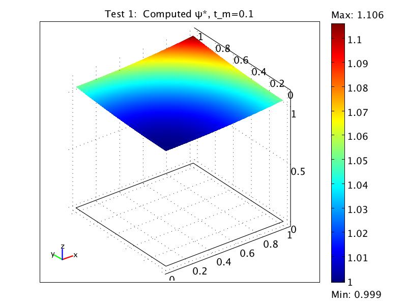
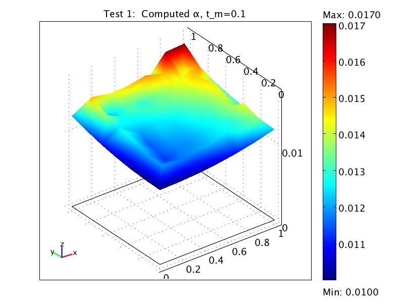
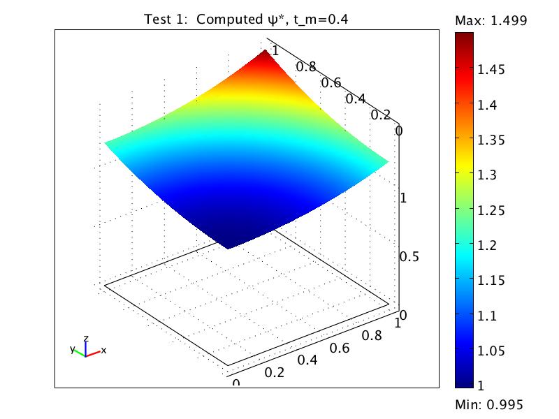
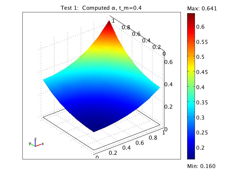
Fig. 2: Computed $\psi^{m}_{h}$ (left) and $\alpha^{m}_{h}$ (right) for Test 1 at $t_{m}=0.1$ (top), $t_{m}=0.4$ (middle), and $t_{m}=1.0$ (bottom). $\Delta t=0.1$, $h=0.05$.

6.2 Test 2

The goal of this test is to calculate the rate of convergence of $\|\psi^{\varepsilon}-\psi_{h}^{\varepsilon}\|$ and $\|\alpha^{\varepsilon}-\alpha^{\varepsilon}_{h}\|$ for a fixed $\varepsilon$ while varying $\Delta t$ and $h$ with the relation $\Delta t=h^{2}$. We solve (45)–(47) but with a new boundary condition: $\frac{\partial\Delta\psi^{\varepsilon}}{\partial\nu}=\phi^{\varepsilon}$. Let $V^{h}_{g_{N}}$ and $W^{h}_{g_{D}}$ be defined in the same way as in Test 1 using the following test functions and parameters

$$c(t) =(\psi^{\varepsilon},1),$$

$$g_{N} =te^{t(x_{1}^{2}+x_{2}^{2})/2}(x_{1}\nu_{x_{1}}+x_{2}\nu_{x_{2}}),$$

$$g_{D} =t^{2}(1+t(x_{1}^{2}+x_{2}^{2}))e^{t(x_{1}^{2}+x_{2}^{2})},$$

$$\qquad-\varepsilon t^{2}e^{t(x_{1}^{2}+x_{2}^{2})/2}(8+8t(x_{1}^{2}+x_{2}^{2})+t^{2}(x_{1}^{2}+x_{2}^{2})^{2}),$$

$$F =t\bigl{(}2+4t(x_{1}^{2}+x_{2}^{2})+t^{2}(x_{1}^{2}+x_{2}^{2})^{2}\bigr{)}e^{t(x_{1}^{2}+x_{2}^{2})}$$

$$\qquad-\frac{\varepsilon t}{2}e^{t(x_{1}^{2}+x_{2}^{2})/2}\bigl{(}32+56(x_{1}^{2}+x_{2}^{2})t+16t^{2}(x_{1}^{2}+x_{2}^{2})^{2}+t^{3}(x_{1}^{2}+x_{2}^{2})^{3}\bigr{)},$$

$$\phi^{\varepsilon} =\bigl{(}\bigl{(}4x_{1}t^{2}+x_{2}t^{3}(x_{1}^{2}+x_{2}^{2})\bigr{)}\nu_{x_{1}}+\bigl{(}4x_{2}t^{2}+x_{2}t^{3}(x_{1}^{2}+x_{2}^{2})\nu_{x_{2}}\bigr{)}\bigr{)}e^{t(x_{1}^{2}+x_{2}^{2})/2},$$

so that the exact solution of (6)–(12) is given by

$$\psi^{\varepsilon}(x,t) =e^{t(x_{1}^{2}+x_{2}^{2})/2},$$

$$\alpha^{\varepsilon}(x,t) =t^{2}(1+t(x_{1}^{2}+x_{2}^{2}))e^{t(x_{1}^{2}+x_{2}^{2})}-\varepsilon t^{2}e^{t(x_{1}^{2}+x_{2}^{2})/2}(8+8t(x_{1}^{2}+x_{2}^{2})+t^{2}(x_{1}^{2}+x_{2}^{2})^{2}).$$

The errors at time $t_{m}=0.25$ are listed in Table 1 and are plotted verses $\Delta t$ in Figure 3. The results clearly indicate that $\|\alpha^{\varepsilon}(t_{m})-\alpha^{m}_{h}\|_{L^{2}}=O(\Delta t)$ and $\|\psi^{\varepsilon}(t_{m})-\psi^{m}_{h}\|=O(\Delta t)$ in all norms as expected by the analysis in the previous section.

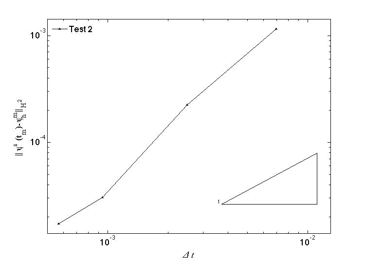
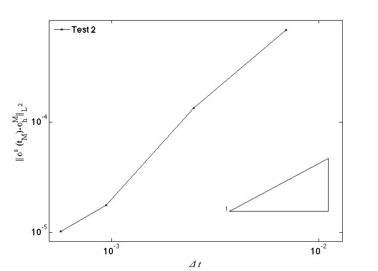
Fig. 3: Test 2: Change of $\|\psi^{\varepsilon}(t_{M})-\psi^{M}_{h}\|$ w.r.t. $\Delta t=h^{2}$. $\varepsilon=0.01$, $t_{m}=0.25$.

$h$	$\Delta t$	$\|\psi^{\varepsilon}(t_{m})-\psi^{m}_{h}\|_{L^{2}}$	$\|\psi^{\varepsilon}(t_{m})-\psi^{m}_{h}\|_{H^{1}}$	$\|\psi^{\varepsilon}(t_{m})-\psi^{m}_{h}\|_{H^{2}}$	$\|\alpha^{\varepsilon}(t_{m})-\alpha^{m}_{h}\|_{L^{2}}$
0.08333	0.00694	0.000214135	0.000978608	0.004434963	0.003456864
0.05	0.0025	6.15715E-05	0.000281367	0.001274611	0.001009269
0.03066	0.00094	1.42185E-05	6.49825E-05	0.000294575	0.000232896
0.02384	0.00057	7.13357E-06	3.25959E-05	0.000147586	0.000116731

Table 1: Change of $\|\psi^{\varepsilon}(t_{M})-\psi^{M}_{h}\|$ w.r.t. $\Delta t=h^{2}$. $\varepsilon=0.01$, $t_{m}=0.25$.

6.3 Test 3

For this test, we solve problem (45)–(47) with domain $U=(0,6)^{2}$ and initial condition

$$\alpha_{0}(x)=\frac{1}{8}\chi_{[2,4]\times[2.25,3.75]}(4-x_{1})(x_{1}-2)(3.75-x_{2})(x_{2}-2.25),$$

where $\chi_{[2,4]\times[2.25,3.75]}$ denotes the characteristic function of the set $[2,4]\times[2.25,3.75]$. We comment that the exact solution of this problem is unknown. We plot the computed $\alpha^{m}_{h}$ and $\psi^{m}_{h}$ at times $t_{m}=0$, $t_{m}=0.05$, and $t_{m}=0.1$, and $t_{m}=0.15$ in Figure 4 with parameters $\Delta t=0.001,\ h=0.05$, and $\varepsilon=0.01$. As expected, the figure shows that $\alpha_{h}^{m}>0$ and $\psi_{h}^{m}$ is convex for all $m$.

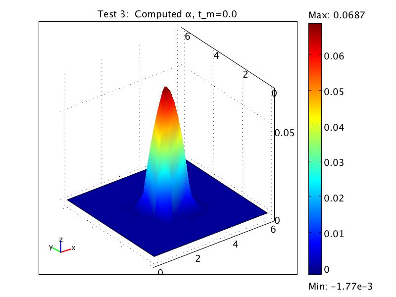
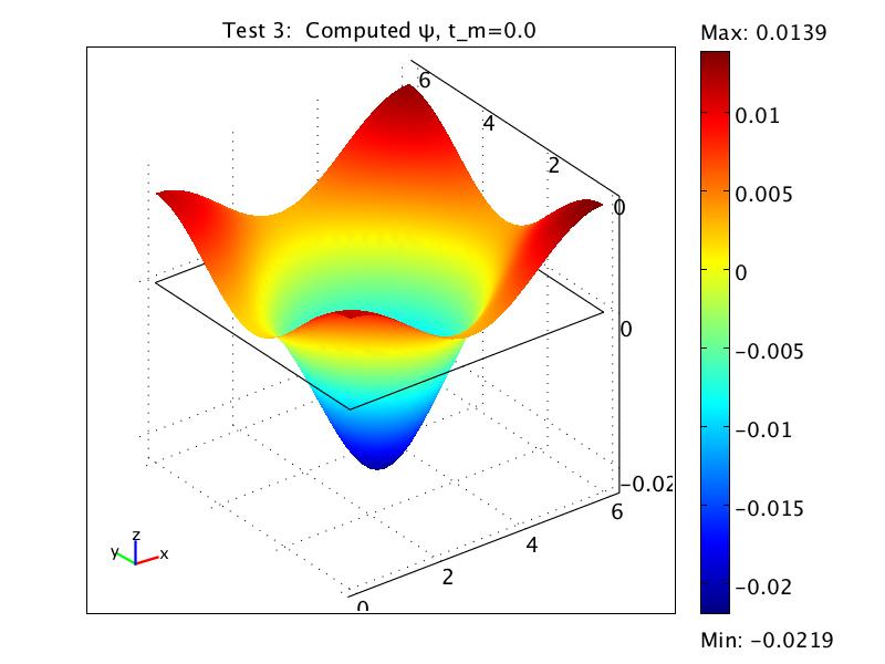
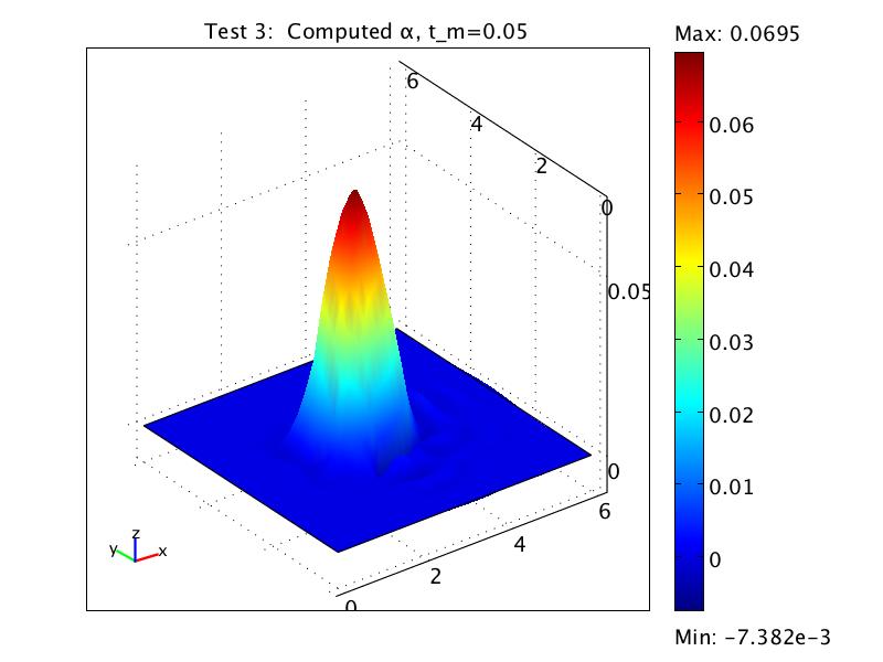
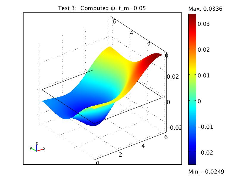
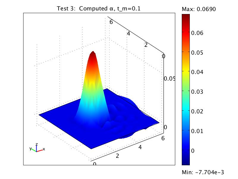
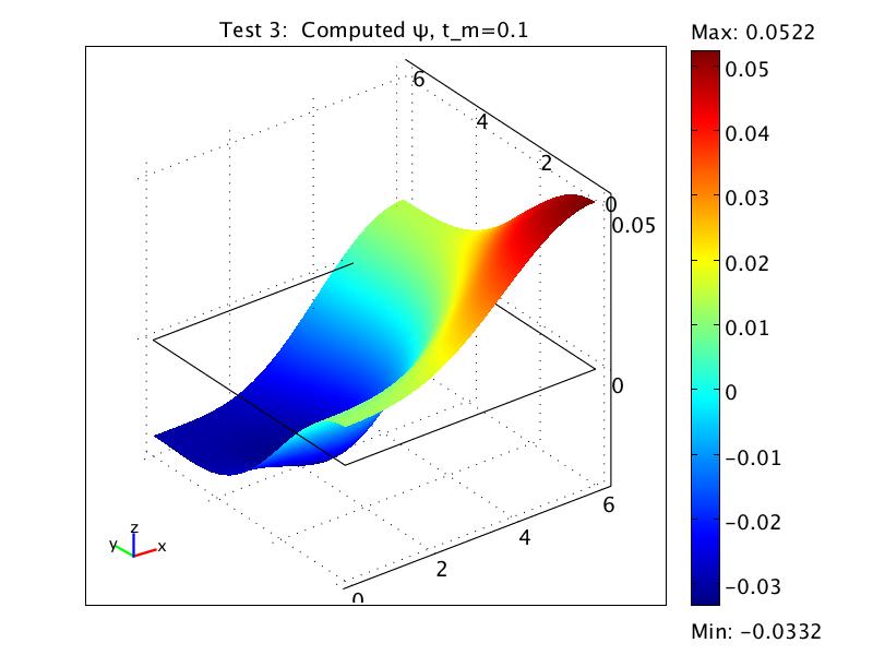
Fig. 4: Test 3: Computed $\alpha^{m}_{h}$ (left) and $\psi^{m}_{h}$ (right) at $t_{m}=0$ (top), $t_{m}=0.05$ (middle), and $t_{m}=0.1$ (bottom). $\Delta t=0.01,\ h=0.05,\ \varepsilon=0.01$

References

• [1] A. D. Aleksandrov, Certain estimates for the Dirichlet problem, Soviet Math. Dokl., 1:1151-1154, 1961.
• [2] G. Barles and P. E. Souganidis, Convergence of approximation schemes for fully nonlinear second order equations, Asymptotic Anal., 4(3):271–283, 1991.
• [3] J. Benamou and Y. Brenier, Weak Existence for the Semigeostrophic Equations Formulated as a Coupled Monge-Ampére/Transport Problem, SIAM. J. Appl. Math., 58(5):1450-1461, 1998.
• [4] S. C. Brenner and L. R. Scott, The Mathematical Theory of Finite Element Methods, second edition, Springer (2002).
• [5] Y. Brenier, Polar factorization and monotone rearrangement of vector-valued functions. Comm. Pure Appl. Math., 44 (1991), pp. 375-417
• [6] L. A. Caffarelli and X. Cabré, Fully Nonlinear Elliptic Equations, volume 43 of American Mathematical Society Colloquium Publications. American Mathematical Society, Providence, RI, 1995.
• [7] L. A. Caffarelli and M. Milman, Monge Ampère Equation: Applications to Geometry and Optimization, Contemporary Mathematics, Vol. 226, American Mathematical Society, Providence, RI, 1999.
• [8] P. G. Ciarlet, The Finite Element Method for Elliptic Problems. North-Holland, Amsterdam, 1978.
• [9] M. G. Crandall, H. Ishii, and P.-L. Lions, User’s guide to viscosity solutions of second order partial differential equations, Bull. Amer. Math. Soc. (N.S.), 27(1):1–67, 1992.
• [10] M. Cullen, R. Douglas, Applications of the Monge-Ampére equation and Monge transport problem to meteorology and oceanography, Contemporary Mathematics, 226:33–53, 1999.
• [11] M. Cullen and M. Feldman, Lagrangian solutions of semigeostrophic equations in physical space, SIAM J. Math. Anal., 37:1371–1395, 2006.
• [12] M. Cullen, J. Norbury, and R. J. Purser, Generalized Lagrangian solutions for atmospheric and oceanic flows, SIAM J. Appl. Math., 51:20–31, 1991.
• [13] E. J. Dean and R. Glowinski, Numerical methods for fully nonlinear elliptic equations of the Monge-Ampère type, Comput. Methods Appl. Mech. Engrg., 195(13-16):1344–1386, 2006.
• [14] J. Douglas, Jr., Numerical Methods for the Flow of Miscible Fluids in Porous Media in Numerical Methods in Coupled Systems (R. W. Lewis, P. Bettess, and E. Hinton eds.), John Wiley & Songs, New York.
• [15] J. Douglas, Jr. and T. Russell, Numerical Methods for Convection-Dominated Diffusion Problems Based on Combining the Method of Characteristics with Finite Element or Finite Difference Procedures, SIAM. J. Numer. Anal., 19(5):871-885, 1982.
• [16] L. C. Evans, Partial Differential Equations, volume 19 of Graduate Studies in Mathematics, American Mathematical Society, Providence, RI, 1998.
• [17] X. Feng, Convergence of the vanishing moment method for the Monge-Ampére equations in two spatial dimensions, Trans. AMS, (submitted)
• [18] X. Feng and M. Neilan, Vanishing moment method and moment solutions for second order fully nonlinear partial differential equations, DOI 10.1007/s10915-008-9221-9, 2008
• [19] X. Feng and M. Neilan, Mixed finite element methods for the fully nonlinear Monge-Ampére equation based on the vanishing moment method, SIAM J. Numer. Anal. (submitted)
• [20] X. Feng and M. Neilan, Analysis of Galerkin methods for the fully nonlinear Monge-Ampére equation, Math. Comp. (submitted)
• [21] D. Gilbarg and N. S. Trudinger, Elliptic Partial Differential Equations of Second Order, Classics in Mathematics, Springer, Berlin, 2001. Reprint of the 1998 edition.
• [22] B. J. Hoskins, The geostrophic momentum approximation and the semigeostrophic equations, J. Atmospheric Sci., 32:233–242, 1975.
• [23] G. Loeper, A Fully Non-linear Version of the Incompressible Euler Equations: The Semi-Geostrophic System, http://arxiv.org/abs/math/0504138v1.
• [24] A. Majda, Introduction to PDEs and Waves for Atmosphere and Ocean, American Mathematical Society, 2003.
• [25] M. Neilan, A nonconforming Morley finite element method for the fully nonlinear Monge-Ampére equation, Numer. Math. (submitted)
• [26] M. Neilan, Numerical Methods for Second Order Fully Nonlinear PDEs, Ph.D. Dissertation, the University of Tennessee (in preparation).
• [27] R. J. McCann and A. M. Oberman. Exact semigeostrophic flows in an elliptical ocean basin, Nonlinearity, 17(5):1891–1922, 2004.
• [28] A. M. Oberman, Wide stencil finite difference schemes for elliptic Monge-Ampére equation and functions of the eigenvalues of the hessian, Discret. Cont. Dynam. Sys. B, 10(1):221-238, 2008.
• [29] V. I. Oliker and L. D. Prussner, On the numerical solution of the equation $(\partial^{2}z/\partial x^{2})(\partial^{2}z/\partial y^{2})-((\partial^{2}z/\partial x\partial y))^{2}=f$ and its discretizations. I., Numer. Math., 54(3):271–293, 1988.
• [30] R. Salmon, Lectures on geophysical fluid dynamics, Oxford University Press, New York, 1998.