Disk masses in the embedded and T Tauri phases of stellar evolution
Abstract
Motivated by a growing concern that masses of circumstellar disks may have been systematically underestimated by conventional observational methods, we present a numerical hydrodynamics study of time-averaged disk masses () around low-mass Class 0, Class I, and Class II objects. Mean disk masses () are then calculated by weighting the time-averaged disk masses according to the corresponding stellar masses using a power-law weight function with a slope typical for the Kroupa initial mass function of stars. Two distinct types of disks are considered: self-gravitating disks, in which mass and angular momentum are redistributed exclusively by gravitational torques, and viscous disks, in which both the gravitational and viscous torques are at work. We find that self-gravitating disks have mean masses that are slowly increasing along the sequence of stellar evolution phases. More specifically, Class 0/I/II self-gravitating disks have mean masses , , and , respectively. Viscous disks have similar mean masses () in the Class 0/I phases but almost a factor of 2 lower mean mass in the Class II phase (). In each evolution phase, time-averaged disk masses show a large scatter around the mean value. Our obtained mean disk masses are larger than those recently derived by Andrews & Williams and Brown et al., regardless of the physical mechanisms of mass transport in the disk. The difference is especially large for Class II disks, for which we find but Andrews and Williams report median masses of order . When Class 0/I/II systems are considered altogether, a least-squares best fit yields the following relation between the time-averaged disk and stellar masses, . The dependence of on becomes progressively steeper along the sequence of stellar evolution phases, with exponents , , and for Class 0, Class I, and Class II systems, respectively.
Subject headings:
circumstellar matter — planetary systems: protoplanetary disks — hydrodynamics — ISM: clouds — stars: formation1. Introduction
It has now become evident that disks of gas and dust are present from the earliest phases of stellar evolution (Class 0 and Class I) and last for at least several million years into the late Class II phase. Disks are observed or inferred around most T Tauri stars and even around brown dwarfs. The evidence for disks around Class 0 and Class I sources is more indirect. In this early phase of stellar evolution, the protostar/disk system is deeply embedded in an envelope – a remnant of the cloud core from which the protostar is forming. Nevertheless, recent observations by Andrews & Williams (2005) suggest that Class I disks have a larger median mass than that of Class II disks.
In spite of a considerable progress in the detection of disks around young stellar objects (YSOs), an accurate determination of disk masses is still challenging. It is difficult to directly determine disk masses from the spectral lines of molecular species because the brightest, easily detectable lines (i.e., the rotational transitions of CO) are optically thick and likely to be severely depleted. Therefore, disk masses are usually inferred from analyzing the spectral energy distribution of YSOs from the mid-infrared through submillimeter bands (e.g. Andrews & Williams, 2005; Brown et al., 2000). Such measurements of disk masses suffer from large uncertainties in the normalization of dust opacities and gas-to-dust ratios, which led Hartmann et al. (2006) to conclude that T Tauri disk masses have been systematically underestimated by conventional analyses.
Another complication arises from poorly known physical processes in the disk. A usual assumption of optically thin circumstellar disks may significantly underestimate disk masses, particularly for objects with larger flux densities. However, a self-consistent treatment of a non-negligible optical depth requires a knowledge of the radial gas surface density profile in the disk (Andrews & Williams, 2005), which may depend significantly on the dominant physical mechanism of mass and angular momentum redistribution in the disk (Vorobyov & Basu, 2008b).
Given large uncertainties in the measurements of disk masses, numerical simulations of self-consistent formation and evolution of circumstellar disks can provide valuable information on disk masses in the early embedded and late phases of YSO evolution. It has been shown in the past that the saturation of spiral gravitational instabilities at a finite amplitude in a self-gravitating, Toomre-unstable disk allows for the steady transport of mass and momentum, which eventually limits disk masses (e.g. Adams et al., 1989; Shu et al., 1990; Laughlin et al., 1997, 1998). In this paper, we perform numerical simulations of the long-term evolution of self-consistently formed circumstellar disks around low-mass stars (). We consider both the self-gravitating disks, in which radial transport of mass and angular momentum is done exclusively via gravitational torques, and viscous disks, which feature gravitational torques as well as viscous ones. We seek to determine numerically the disk masses in the Class 0, Class I, and Class II phases of stellar evolution.
The paper is organized as follows. The numerical methods and initial parameters of cloud cores are given in § 2. Our obtained masses for self-gravitating and viscous disks are presented in § 3 and § 4. We compare our numerical results with observations in § 5. The model and numerical caveats are discussed in § 6. The main results are summarized in § 7.
2. Description of numerical methods
We use the thin-disk approximation to compute the evolution of rotating, gravitationally bound cloud cores. This allows efficient calculation of the long-term evolution of a large number of models. We start our numerical integration in the pre-stellar phase, which is characterized by a collapsing starless cloud core, and continue into the main accretion phase, which sees the formation of a central star and circumstellar disk. We cover all major phases of the evolution of a YSO, starting from its formation and ending with the T Tauri phase. The integration ends when the age of the central star is about three million years. In some models we extend the integration up to 5 Myr. We emphasize that circumstellar disks are formed self-consistently in our numerical simulations, rather than being introduced as an initial parameter of the model.
Once the disk is formed, its mass is determined by an interplay between the efficiency of the mass and angular momentum transport in the disk111In fact, disks may also transport angular momentum to the external environment due to magnetic braking. This effect will be considered in a follow-up paper. and the infall rate of matter from the surrounding envelope onto the disk. At the time of disk formation, the infall rates take values between yr-1 and yr-1 (measured at AU) for the least and most massive cloud cores, respectively, but they show a fast decline with time. These values (and strong time variation) are consistent with the infall rates derived by Klessen (2001) using numerical models that follow molecular cloud evolution from turbulent fragmentation toward the formation of stellar clusters. We note that once the disk is formed, the infall rate of matter from the envelope onto the disk is not necessarily the same as the mass accretion rate from the disk onto the protostar. While the former shows a fast decline with time, the latter is usually characterized by a much slower decline and has a strong dependence on the stellar mass (Vorobyov & Basu, 2007, 2008a).
We use two numerical approaches: a basic approach that accounts for the radial transport due to gravitational toques and a viscous approach that accounts for the radial transport due to both the gravitational torques and viscosity. Gravitational torques are known to efficiently redistribute mass and angular momentum in circumstellar disks (e.g. Lodato & Rice, 2004, 2005). They were shown to play an important role in driving the FU-Ori-like bursts in the early embedded phase of disk evolution (Vorobyov & Basu, 2005b, 2006). In the late disk evolution, negative gravitational torques associated with low-amplitude azimuthal density perturbations in the disk can drive mass accretion rates that are consistent with those measured in the intermediate and upper-mass T Tauri stars (Vorobyov & Basu, 2007, 2008a).
2.1. Basic numerical approach
In the basic numerical approach, the collapse of a cloud core and subsequent evolution of a star/disk system is carried out by solving the basic equations of mass and momentum transport in the thin-disk approximation (see e.g. Vorobyov & Basu, 2006)
| (1) | |||||
| (2) |
where is the mass surface density, is the vertically integrated form of the gas pressure , is the radially and azimuthally varying vertical scale height, is the velocity in the disk plane, is the gravitational acceleration in the disk plane, and is the gradient along the planar coordinates of the disk. The gravitational acceleration is found by solving for the Poisson integral (see Vorobyov & Basu, 2006). The fact that we account for the disk self-gravity means that gravitational torques arise self-consistently in our numerical simulations and not imitated by some means of -viscosity.
Taking into account the complexity of gas thermodynamics in circumstellar disks (see § 6), we have adopted a barotropic equation of state that closes equations (1) and (2) and makes a transition from isothermal to adiabatic evolution at g cm-2
| (3) |
where is the isothermal sound speed, the value of which is set equal to that of the initial cloud core, and . Equation (3), though neglecting detailed cooling and heating processes, was shown to reproduce to a first approximation the radial temperature gradients in the disk (Vorobyov & Basu, 2007) and the density-temperature relation for collapsing cloud cores derived by Masunaga & Inutsuka (2000) using a detailed radiation hydrodynamics simulation (Vorobyov & Basu, 2006).
The vertical scale height is determined assuming the local hydrostatic equilibrium in the gravitational field of a disk and central star (Vorobyov & Basu, 2008b). The relevant formulas are given in the Appendix.
2.2. Viscous numerical approach
Viscosity is another important mechanism of angular momentum and mass redistribution in astrophysical disks. Most analytical and numerical studies of viscous evolution of thin circumstellar disks have employed the standard axisymmteric model of Lynden-Bell & Pringle (1974), in which the surface density of a Keplerian disk evolves with time according to the following diffusion equation
| (4) |
where is the kinematic viscosity.
In the present paper, we take a more fundamental approach and describe the effect of (yet unspecified) viscosity in terms of the classic viscous stress tensor
| (5) |
where is a symmetrized velocity gradient tensor, is the unit tensor, and is the dynamical viscosity. This approach allows for a self-consistent treatment of both, self-gravity and viscosity, within the same numerical formalism. The resulting mass and momentum transport equations in the viscous numerical approach are
| (6) | |||||
| (7) |
where is the divergence of the rank-two viscous stress tensor . The relevant components of are given in the Appendix. Equations (6) and (7) are closed with the barotropic equation of state (3). We note that the viscous approach accounts self-consistently for both the gravitational and viscous torques which may arise during numerical simulations.
It is evident that the practical application of equation (7) requires a knowledge of the dynamical viscosity of the disk. Unfortunately, our understanding of viscous processes in circumstellar disks is still incomplete. We know that molecular (collisional) viscosity is most certainly too low to be of practical interest. Turbulence driven by the magneto-rotational instability (MRI) is a most promising source of viscosity at present (Balbus & Hawley, 1991), though other mechanisms cannot be ruled out completely.
In this paper, we make no specific assumptions as to the source of viscosity and define the coefficient of dynamical viscosity using the usual -prescription of Shakura & Sunyaev (1973)
| (8) |
where spatially and temporally uniform is set equal to 0.01 and is the effective sound speed. Our numerical simulations of embedded and T Tauri disks indicate that yields disk sizes and radial slopes that are in general agrement with observations (Vorobyov & Basu, 2008b). Lower values of () have little effect on the evolution of self-gravitating disks, whereas substantially higher values () quickly destroy the disks. Hartmann et al. (1998) also predicted similar values for by analyzing accretion rates in T Tauri disks. Since viscosity in our model is assumed to arise due to some physical processes in the disk, we keep equal to zero during the early “pre-disk” phase of evolution and set equal to 0.01 only when a circumstellar disk forms around a central star.
2.3. Initial condition
The initial radial distributions of surface density and angular velocity in our model cloud cores are those characteristic of a collapsing axisymmetric magnetically supercritical core (Basu, 1997)
| (9) |
| (10) |
where is the radial scale length defined as and . These initial profiles are characterized by the important dimensionless free parameter and have the property that the asymptotic () ratio of centrifugal to gravitational acceleration has magnitude (see Basu, 1997). The centrifugal radius of a mass shell initially located at radius is estimated to be , where is the specific angular momentum. Since the enclosed mass is a linear function of at large radii, this also means that . The gas has a mean molecular mass and cloud cores are initially isothermal with temperature K.
We present results from three sets of models, each with a different value of . The standard model has based on typical values km s-1, g cm-2, and km s-1 pc-1. The outer radius is taken to be pc, and the total cloud mass is . Other models with but different mass (outer radius) are generated by varying and so that their product is constant. Note that, when is varied, has to be changed accordingly. All clouds are characterized by the same ratio . To generate the second set of models, , we set km s-1 pc-1 and all other quantities the same as in the standard model with . Models of varying mass are then generated in the same manner as for the models. The third set of models, with , are also obtained in this way, by first using km s-1 pc-1. Overall, there are 7 models with , 13 models with , and 12 with . The range of initial cloud masses () amongst our models is . The parameters of our models are listed in Table 1 (), Table 2 (), and Table 3 (). We note that our model values of km s-1 pc-1 are within a typical range of velocity gradients measured in dense starless cores by Caselli et al. (2002).
| Model | |||||
|---|---|---|---|---|---|
| 1 | 1209 | 0.13 | 1.14 | 7186 | 0.7 |
| 2 | 1382 | 0.12 | 1.0 | 8213 | 0.8 |
| 3 | 1728 | 0.093 | 0.8 | 10266 | 0.98 |
| 4 | 2074 | 0.077 | 0.67 | 12320 | 1.18 |
| 5 | 2937 | 0.055 | 0.47 | 17452 | 1.67 |
| 6 | 4147 | 0.039 | 0.33 | 24640 | 2.36 |
| 7 | 5184 | 0.031 | 0.27 | 30800 | 2.95 |
| Model | |||||
|---|---|---|---|---|---|
| 8 | 622 | 0.26 | 3.1 | 3696 | 0.35 |
| 9 | 691 | 0.23 | 2.8 | 4106 | 0.4 |
| 10 | 864 | 0.19 | 2.24 | 5133 | 0.5 |
| 11 | 1037 | 0.16 | 1.87 | 6160 | 0.6 |
| 12 | 1210 | 0.13 | 1.6 | 7187 | 0.7 |
| 13 | 1417 | 0.11 | 1.4 | 8213 | 0.8 |
| 14 | 1728 | 0.093 | 1.12 | 10267 | 0.98 |
| 15 | 2454 | 0.065 | 0.79 | 14579 | 1.4 |
| 16 | 2765 | 0.058 | 0.7 | 16428 | 1.57 |
| 17 | 3456 | 0.046 | 0.56 | 20533 | 1.97 |
| 18 | 3802 | 0.042 | 0.51 | 22587 | 2.16 |
| 19 | 4147 | 0.038 | 0.47 | 24640 | 2.36 |
| 20 | 4838 | 0.033 | 0.4 | 28747 | 2.75 |
| Model | |||||
|---|---|---|---|---|---|
| 21 | 518 | 0.31 | 4.53 | 3080 | 0.3 |
| 22 | 691 | 0.23 | 3.4 | 4106 | 0.4 |
| 23 | 864 | 0.19 | 2.7 | 5133 | 0.5 |
| 24 | 1037 | 0.16 | 2.26 | 6160 | 0.6 |
| 25 | 1210 | 0.13 | 1.94 | 7187 | 0.7 |
| 26 | 1417 | 0.11 | 1.7 | 8213 | 0.8 |
| 27 | 2073 | 0.077 | 1.13 | 12320 | 1.18 |
| 28 | 2420 | 0.066 | 0.97 | 14373 | 1.38 |
| 29 | 3283 | 0.049 | 0.72 | 19506 | 1.87 |
| 30 | 3802 | 0.042 | 0.62 | 22587 | 2.16 |
| 31 | 4147 | 0.039 | 0.57 | 24640 | 2.36 |
| 32 | 4493 | 0.036 | 0.52 | 26693 | 2.56 |
2.4. Numerical technique
Hydrodynamic equations of the basic and viscous numerical models are solved in polar coordinates on a numerical grid with points. We use the method of finite differences with a time-explicit, operator-split solution procedure. Advection is performed using the second-order van Leer scheme. The radial points are logarithmically spaced. The innermost grid point is located at AU, and the size of the first adjacent cell lies in the range between 0.26 AU (model 21) and 0.36 AU (model 7). It means that the ratio of the cell size to radius is constant for a given cloud core and varies from (model 21) to (model 7).
We introduce a “sink cell” at AU, which represents the central star plus some circumstellar disk material, and impose a free inflow inner boundary condition. About 95 per cent of the material crossing the inner boundary lands into the star, the rest constitutes an inner circumstellar region of constant surface density. The dynamics of the inner region ( AU) is not computed but it contributes to the total gravitational potential of the system. We do not account for a possible mass loss from the sink cell due to stellar jets, since our model is two-dimensional and it is not clear how the mass ejection efficiency varies with stellar age. The outer boundary is such that the cloud has a constant mass and volume. More details on numerical techniques and relevant tests are given in Vorobyov & Basu (2006).
3. Masses of self-gravitating disks
In this section we present disk masses obtained using the basic numerical approach described in § 2.1. In the framework of this numerical model, disk masses are controlled by the rate of mass infall from the surrounding envelope and the radial transport of mass and angular momentum due to gravitational torques. No viscous torques are present in this case.
An accurate determination of disk masses in numerical simulations of collapsing cloud cores is not a trivial task. Self-consistently formed circumstellar disks have a wide range of masses and sizes, which are not known a priori. However, numerical and observational studies of circumstellar disks indicate that the disk surface density is a declining function of radius. Therefore, we distinguish between disks and infalling envelopes using a critical surface density for the disk-to-envelope transition, for which we choose a value of g cm-2. This choice is dictated by the fact that densest starless cores have surface densities only slightly lower than the adopted value of . In addition, our numerical simulations indicate that self-gravitating disks have sharp outer edges and the gas densities of order g cm-2 characterize a typical transition region between the disk and envelope (Vorobyov & Basu, 2007).
To compare disk masses in three distinct phases of stellar evolution we need an evolutionary indicator to distinguish between Class 0, Class I, and Class II phases. We use a classification of André et al. (1993), who suggest that the transition between Class 0 and Class I objects occurs when about of the initial cloud core is accreted onto the protostar/disk system. The Class II phase is consequently defined by the time when the infalling envelope clears and its total mass drops below 10% of the initial cloud core mass . It should be mentioned here that there exists no unique classification scheme for protostars. For instance, Vorobyov & Basu (2005a) have proposed a classification scheme that hinges on a temporal behaviour of bolometric luminosity . They identify Class 0 phase with a period of temporally increasing and Class I phase with a later period of decreasing . The peak in corresponds to the evolutionary time when per cent of the cloud core mass has been accreted by the protostar. Observers prefer to classify protostars by their spectral energy distributions. For instance, Lada (1987) and Andrews & Williams (2005) use the values of power-law index (defined by , where is the infrared flux density at frequency ) to distinguish between Class I and Class II objects. André et al. (1993) use the ratio of submillimeter to bolometric luminosity for the same purposes. Although these classifications are physically related, it is possible that they may differ from our adopted classification, especially if some of the gas is removed from the cloud core and does not accrete. We acknowledge that the difference in the existing classification schemes may systematically shift our results.
3.1. Temporal evolution of self-gravitating disks
We start by comparing the long-term evolution of disk masses in four sample models, which are chosen to represent a full spectrum of the initial cloud core masses with a constant ratio of centrifugal to gravitational acceleration. Figure 1 shows the disk masses (thick solid lines), stellar masses (thin solid lines), and envelope masses (dashed lines) in model 8 (upper left, ), model 11 (upper right, ), model 16 (lower left, ), and model 20 (lower right, ). The horizontal axis is the time elapsed since the formation of a central star. All masses are calculated relative to the corresponding initial cloud core mass . The vertical dotted lines mark the onset of Class I (left) and Class II (right) phases.
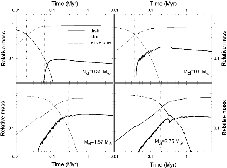
Our numerical simulations demonstrate that cloud cores with constant (but different size) form disks roughly at the same physical time after the formation of a central star but in distinct stellar evolution phases. For instance, model 8 starts to build a disk in the late Class I phase, while model 20 does that in the midst of Class 0 phase. Cloud cores of greater mass tend to form disks in the earlier phase of stellar evolution than their low-mass counterparts.
The upper panel of Fig. 1 identifies cases when Class 0 stars have no disks associated with them. We emphasize here that due to the use of the sink cell in our numerical code we can resolve only those disks whose outer radii are larger than 5 AU. It means that even though circumstellar disks do not form around some Class 0 objects in our numerical simulations, as in models 8 and 11 (top panels in Fig. 3), one may suppose that such disks still exist but their size is simply smaller than that of the sink cell. Our test runs with a sink cell set to 0.5 AU (instead of 5 AU) confirm that disks indeed forms earlier in the evolution but quickly expands to 5 AU and beyond. Hence, the absence of disks around some Class 0 objects may be to some extent caused by a finite-size sink cell. However, it is still possible that some Class 0 objects have no disks associated with them. This is particularly true for those objects that develop from cloud cores with low rates of rotation, since in this case a (substantial) portion of the disk material will be characterized by the centrifugal radius (estimated as ) that is smaller than the radius of the protostar, . A numerical code with realistic treatment of the protostar formation is needed to accurately address this issue.
Another interesting feature of self-gravitating disks that can be seen in Fig. 1 is that the disk-to-star mass ratio never exceeds some characteristic value, approximately , irrespective of the initial cloud core mass. This is rather counterintuitive. For instance, models 16 and 20 (bottom panels in Fig. 1) form disks in the Class 0 phase, which is characterized by envelope masses that are considerably greater than those of the protostars. As a consequence, one may expect the formation of a disk with mass that is at least comparable to or even greater than that of a protostar. It turns out, however, that circumstellar disks that form in the Class 0 or early Class I phase around stars with mass develop vigourous gravitational instability – a very efficient means of inward mass transport that helps keep the disk mass well below that of the protostar. Sharp drops in the disk mass (or equivalent surges in the stellar mass) seen in the upper right and bottom panels of Figure 1 are a manifestation of this process (see e.g. Vorobyov & Basu, 2005b, 2006). Kratter et al. (2008) also predict that disks around stars with mass greater than are expected to be vigorously gravitationally unstable in the early embedded phase of disk evolution. The late evolution phase (Class II) sees only an insignificant decline of disk mass with time.
3.2. Disk masses versus stellar masses
We use 32 models, the parameters of which are listed in Tables 1-3, to analyse the statistical relations between time-averaged disk and stellar masses in the Class 0/I/II evolution phases. Time averaging is performed separately for each evolution phase over the duration of the phase. The age of the oldest disk in our sample is about 3 Myr. Since disk masses in the Class II phase have a tendency to decline with time and the actual lifetime of Class II objects may be longer, we expect that we might have somewhat overestimated disk masses around Class II objects. This, obviously, does not effect our estimates of Class 0/I disk masses.
Figure 2 shows time-averaged disk masses (right column) and time-averaged disk-to-star mass ratios (left column) versus time-averaged stellar masses for Class 0 (open triangles), Class I (filled squares) and Class II objects (plus signs). Several interesting conclusions can be drawn by analysing the figure.
-
1.
Time-averaged disk and stellar masses ( and , respectively) in models with the same ratio of rotational to gravitational acceleration fall onto a unique evolutionary track in the diagram.
-
2.
Class 0 objects occupy the lower-left part of each evolutionary track. No stars with have Class 0 disks (but they have Class I/II disks). In other words, only low-mass stars (within our range of interest, ) can harbour Class 0 disks.
-
3.
Stars of equal mass have disks with similar masses, regardless of the stellar evolution phases.
-
4.
In each stellar evolution phase, disk-to-star mass ratios tend to have greater values for stars of greater mass. However, there is a clear saturation effect for stars with masses greater than – disk masses never grow above of the stellar masses, even for models with the largest values of . The saturation of disk-to-star mass ratios is caused by the onset of vigorous gravitational instability in circumstellar disks that form in the Class 0 and early Class I phase.
| disk type | ||||||
|---|---|---|---|---|---|---|
| self-gravitating | 0.09 | 0.10 | 0.12 | |||
| viscous | 0.10 | 0.11 | 0.06 |
We summarize the main properties of our model self-gravitating disks in Table 4. In order to facilitate the comparison of our numerical results with observations, we calculate mean disk masses (in each evolution phase) by weighting the time-averaged disk masses according to the corresponding stellar masses. The relative importance of the stellar masses is calculated using the following power-law weight function
| (11) |
The slope of is typical for the Kroupa initial mass function (IMF) of stars (Kroupa, 2001). The mean disk masses are then calculated as follows
| (12) |
where and are the time-averaged disk and stellar masses in the -th model (see Fig. 2) and index “ph” stands for Class 0 (C0), Class I (CI), or Class II (CII) stellar evolution phases. The summation is performed separately for each evolution phase. In particular, there are models that have Class 0 disks and models that have Class I disks. All 32 models have Class II disks, of course. The ratio of the normalization constants needed to evaluate equation (12) is found using the continuity condition at .
Table 4 indicates that the mean masses slightly increase along the stellar evolution sequence from around Class 0 objects to around Class II objects. The minimum and maximum time-averaged disk masses ( and , respectively) in each evolution phase are shown in the last three columns of Table 4. It is seen that both the Class I and Class II disks have a similar range of masses, while Class 0 disks have a somewhat narrower range. The smallest time-averaged mass of a self-gravitating disk found in our numerical simulations is .
4. Masses of viscous disks
In this section we present disk masses obtained in the framework of the viscous numerical approach described in § 2.2. We seek to determine the effect of viscosity, and associated viscous torques, on the masses of self-consistently formed circumstellar disks. Our comparison study of viscous versus self-gravitating disks have shown that viscous disks may lack a sharp transition boundary between the disk and the envelope (Vorobyov & Basu, 2008b). This smearing of the disk’s outer physical boundary is particularly pronounced in disks of low mass and in the late Class II phase. In this situation, it is somewhat arbitrary to adopt a value of g cm-2 for the disk-to-envelope transition. Nevertheless, we have recalculated disk masses with g cm-2 and found that this can increase masses of Class II disks by at most. Class 0/I disks are unaffected by the value of , since they usually have sharp outer physical boundaries.
4.1. Temporal evolution of viscous disks
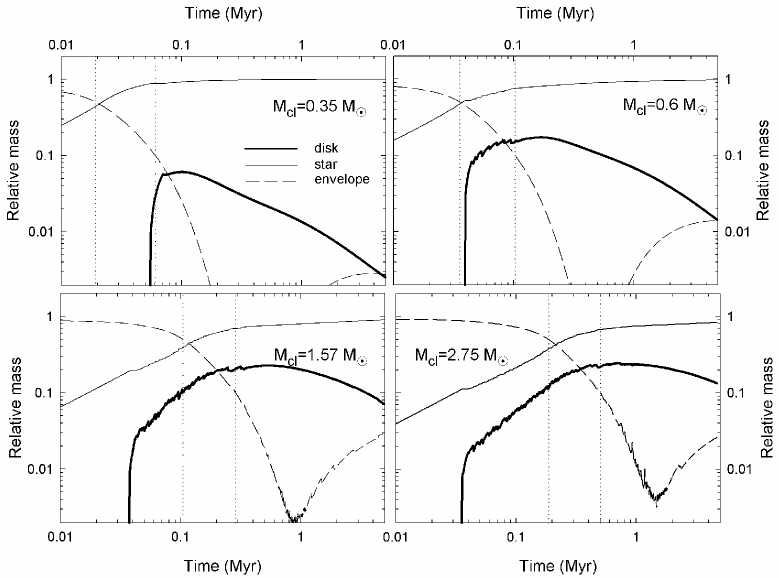
In order to investigate the temporal evolution of viscous disks, we consider the same four sample model cloud cores as in § 3.1. Figure 3 presents disk masses (thick solid lines), stellar masses (thin solid lines), and envelope masses (dashed lines) in model 8 (upper left), model 11 (upper right), model 16 (lower left), and model 20 (lower right). The horizontal axis is time elapsed since the formation of a central star. All masses are calculated relative to the corresponding initial cloud core mass . The vertical dotted lines mark the onset of Class I phase (left line) and Class II phase (right line).
The comparison of Figures 1 and 3 reveals a major difference between self-gravitating and viscous disks – the latter have considerably smaller masses in the late Class II phase than the former. For instance, model 8 in Figure 1 has a final ( Myr) stellar mass and disk mass , while the same model in Figure 3 has . Such a large contrast, however, diminishes for stars of greater mass. For instance, model 16 in Figure 1 has and , while the same model in Figure 3 has . On the other hand, both the viscous and self-gravitating disks have comparable masses in the Class 0/I phases. Even the early Class II phase sees little difference between the masses of viscous and self-gravitating disks, provided that the disks are formed from molecular cloud cores of similar mass. Figure 3 indicates that a small portion of the viscous disk material returns to the envelope in the late disk evolution. This is because we have imposed a fixed gas column density threshold for the disk-to-envelope transition, but viscous disks expand in the late evolution due to the action of viscous torques, which are in fact positive in the outer disk regions (Vorobyov & Basu, 2008b). This numerical effect may slightly reduce the resulted viscous disk masses in the Class II phase.
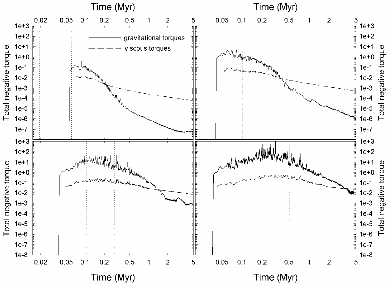
Why does the late stellar evolution phase reveal such a noticeable difference in the disk masses (and, consequently, in disk-to-star mass ratios) between viscous and self-gravitating disks and why is there little difference in the earlier phases? The reason for that can be understood if we consider the temporal evolution of viscous and gravitational torques in the disk. Figure 4 shows total negative torques due to disk self-gravity (, solid lines) and viscosity (, dashed lines) in our four typical models: model 8 (upper left), model 11 (upper right), model 16 (lower left), and model 20 (lower right). The horizontal axis shows time elapsed since the formation of a central star. The total negative torque is computed by summing up local negative torques in each computational zone occupied by the disk. In particular, is computed as a sum of , where and are the gas mass and gravitational potential in a cell with polar coordinates , respectively. The total negative viscous torque is calculated in a similar manner by summing up all local negative viscous torques , where is the surface area occupied by a cell with polar coordinates (). The local torques and are actually the local azimuthal components of the corresponding forces, acting on a fluid element with mass , multiplied by the arm .
Figure 4 indicates that gravitational torques always prevail over viscous torques in the Class 0 and Class I phases. As a result, the disk mass in these phases is determined by the interplay between the mass load from an infalling envelope and the rate of mass and angular momentum transport in the disk due to gravitational torques. In the Class II phase, the strength of gravitational torques diminishes, partly due to a stabilizing influence of a growing central star and partly due to the exhausted mass reservoir in the infalling envelope. As a result, viscous torques, the strength of which shows only a mild decline with time, take a leading role in the Class II phase. They act to further decrease the disk mass when gravitational torques fail to do so.
The actual time in the Class II phase when become greater than is distinct for models with different initial cloud core masses (but similar ratios of rotational to gravitational acceleration ). Low-mass cloud cores form disks late in the evolution (see e.g. model 8 in Fig. 3). The resulting disks have low masses, merely due to the fact that most of the cloud core material has already been accreted directly onto the protostar in the pre-disk phase. As a result, gravitational instability is underdeveloped and viscous torques quickly take over the gravitational ones in the beginning of the Class II phase. Conversely, high-mass cloud cores form disks early in the evolution (see e.g. model 16 and 20 in Fig. 3). The resulting disks are characterized by considerable masses. As a consequence, gravitational torques prevail over viscous torques throughout a considerable portion of the Class II phase. The interested reader is referred to Vorobyov & Basu (2008a, b) for a detailed discussion on gravitational torques and appearances of self-gravitating and viscous disks.
4.2. Relation between disk and stellar masses
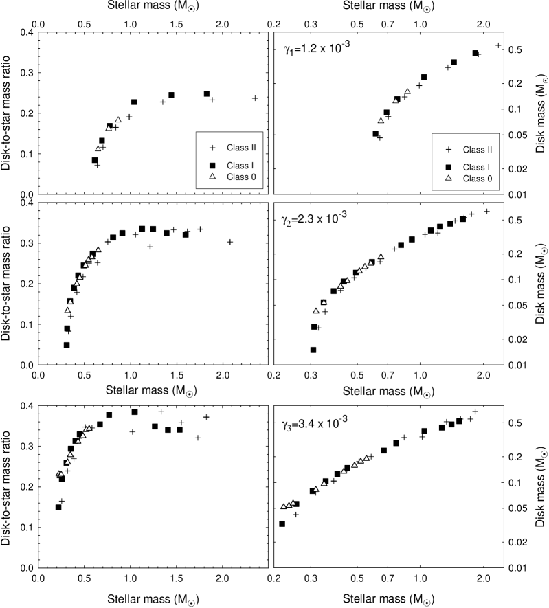
In this section we derive statistical relations between time-averaged disk masses (), time-averaged stellar masses () , and time-averaged disk-to-star mass ratios () for viscous disks in each stellar evolution phase. Time averaging is performed separately in each evolution phase over the duration of the phase. Figure 5 shows (right column) and (left column) versus for Class 0 objects (open triangles), Class I objects (filled squares) and Class II objects (plus signs). The top-to-bottom rows show the data for models with , , and , respectively.
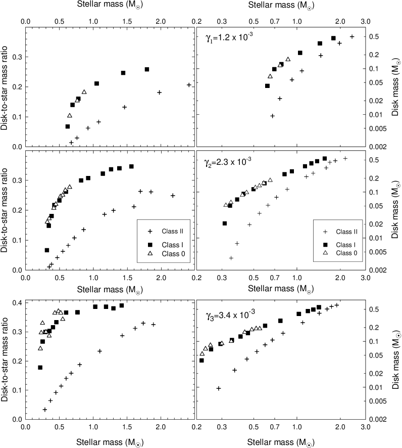
The comparison of Figures 2 and 5 reveals a distinct feature of viscous disks around objects of equal stellar mass – Class II disk have systematically lower masses than their Class 0/I counterparts. This is in sharp contrast to self-gravitating disks studied in § 3 where we have found that Class O/I/II objects with equal stellar mass possess self-gravitating disks of essentially similar mass (see Fig. 2). The difference in masses between Class II and Class 0/I viscous disks is considerable for low-mass stars (up to a factor of 10), but it diminishes for stars of greater mass. However, we have to keep in mind that low-mass stars are statistically more important than their high-mass counterparts.
The dependence of on in Figure 5 is similar to that of Figure 2 – stars of greater mass tend to have greater disk-to-star mass ratios. However, as for the case of disk masses, Class II viscous disks have disk-to-star mass ratios that are lower than those of self-gravitating disks. For instance, the smallest in self-gravitation disks (Fig. 2) is 0.05, while viscous disks have as small as 0.01.
It is interesting to compare our results with the recent work of Kratter et al. (2008), who use semi-analytical models to describe the time evolution of embedded, accreting protostellar disks. As in our model, they account for disk self-gravity and MRI-induced viscosity but also include the effect of stellar and envelope irradiation. They obtain maximum disk-to-star mass ratios in the Class I phases of order , in excellent agreement with our results. The disk mass in their fiducial model shows a temporal behaviour similar to that shown in the lower-left panel of Fig. 3 – it grows in the Class 0 phase, reaches a maximum in Class I phase, and declines afterwards. They also predict that higher mass stars have relatively more massive disks and this trend is expected to extend to stellar masses much greater than those considered in our work ().
We calculate the mean masses of viscous disks using equation (12) and summarize the main properties of our viscous disks in Table 4. It is evident that the range of time-averaged masses and the values of mean masses are quite similar in both the self-gravitating and viscous disks. The latter tend to have slightly larger mean disk masses in the Class 0/I phases, which is explained by the fact that viscous torques tend to oppose gravitational ones in the early disk evolution (Vorobyov & Basu, 2008b). The only significant difference comes from Class II viscous disks, which have a factor of two lower mean mass, , than that of self-gravitating disks. Class II viscous disks also feature the lowest time-averaged disk mass found in our numerical simulations, .
Finally, we seek to determine the relation between time-averaged disk and stellar masses in each stellar evolution phase separately and for the three phases taken altogether. Figure 6 shows versus for our 32 model cloud cores. In particular, the open triangles, filled squares, and plus signs show the data for the Class 0, Class I, and Class II phases, respectively. It is evident that the upper-mass stars have a considerably narrower scatter in disk masses than the lower-mass stars. The least-squares best fit to all data in Figure 6 (solid line) yields the following relation between time-averaged stellar and disk masses (in ) for the three phases taken altogether
| (13) |
The relation between time-averaged disk and stellar masses in each stellar evolution phase is, however, quite different from that expressed by equation (13). The least-squares best fits performed separately for each evolution phase yield the following relations
| (14) | |||||
| (15) | |||||
| (16) |
where indices CO, CI, and CII refer to the Class 0, Class I, and Class II phases, respectively. The dependence of disk masses on stellar masses becomes progressively steeper along the sequence of stellar evolution phases.
The above relations between time-averaged stellar and disk masses were derived for viscous disks, in which both viscosity and self-gravity are at work. Purely self-gravitating disks (zero viscosity) have a similar relation between time-averaged disk and stellar masses when all stellar evolution phases are considered altogether, namely equation (13). However, when each phase is taken separately, the exponents are different from those derived for viscous disks in equations (14)-(16). To avoid confusion, we provide here the relations for viscous disks only, since we believe that some sort of viscosity should be present in circumstellar disks.
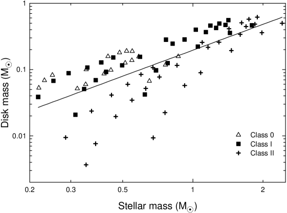
Observations provide conflicting evidence as to the relation between disk and stellar masses in YSOs. For instance, Natta et al. (2001) found a marginal correlation between disk and stellar masses, albeit with a substantial dispersion. On the other hand, Andrews & Williams (2005) claimed no correlation. The correlation in Figure 6 can be broken if a large population of objects occupies both the upper-left and lower-right portions of the diagram. While the latter is feasible due to the incompleteness of our sample of model cloud cores (we have not considered sufficiently low values of the ratio ), the former is unlikely due to the saturation of disk masses discussed in the context of Figure 2 and earlier considered by Adams et al. (1989) and Shu et al. (1990) . No stars can harbour disks with masses comparable to or greater than the stellar mass! It is likely that the uncertainty in disk measurements may introduce a considerable scatter to the observational data which precludes the correlation analysis.
5. Discussion
There exist a growing concern that disk masses around YSOs may be systematically underestimated by conventional observational methods. The simplest argument in favour of this conjecture is a high frequency of detection of Jupiter-like exosolar planets. Both the core accretion and gravitational instability models require disk masses of order for Jupiter-like planets to form, which is about an order of magnitude higher than median disk masses inferred by Andrews & Williams (2005) (hereafter, AW). Another argument in favour of fairly massive disks is the fact that resolved disks show rich non-axisymmetric structures, such as multiple spiral arms or arcs in the case of AB Aurigae (Fukagawa et al., 2004; Grady et al., 1999) and HD 100546 (Grady et al., 2001). Such structures are difficult to sustain in low-mass disks. To remind the reader, a companion star or giant planet would most likely trigger a two-armed spiral response in the disk of a target and not a flocculent multi-arm structure.
As was discussed in the Introduction, measurements of disk masses suffer from the uncertainties in dust opacities and disk radial structure, which could lead to a substantial underestimate of disk masses (e.g. Hartmann et al., 2006). Alternatively, the disk may mask itself, especially late in the evolution, by locking a significant amount of its mass in the form of large dust grains or planetesimals which are inefficient emitters at submillimeter wavelengths (Andrews & Williams, 2005).
Our numerical modeling supports the supposition of Hartmann et al. (2006) that circumstellar disks are more massive than currently inferred from observations. The mean masses of disks in our models range between for Class I objects and for Class II objects, well in excess of the AW’s median masses for either Class I disks () or, especially, Class II disks (). Much the same, our Class 0 disks have mean masses , while five Class 0 disks in a sample of Brown et al. (2000) have a mean mass of order , though the statistics in the case of Class 0 objects is inadequate to draw any firm conclusions.
A closer look at the data provided by AW reveals that our numerical modeling fails to reproduce only the lower bound on the measured disk masses but succeeds at reproducing the upper bound. For instance, figure 15 of AW indicates that Class I disk masses lie in the range , while our Class I disks have masses in the range . Similarly, AW’s Class II disk masses lie in the range , while our disks have masses in the range . If disk masses are indeed systematically underestimated by conventional observational methods, then low-mass disks should suffer from this problem to a greater extent than do upper-mass disks. The reason for this is not well understood.
It is worth noting that our Class 0 disk have masses that are similar to those of Class I disks. This is in agreement with the modeling of circumstellar envelope dust emission of 6 deeply embedded systems by Looney et al. (2003), who have found that Class 0 systems do not have disks that are significantly more massive than those in Class I systems. This led them to conclude that the disk in Class 0 systems must quickly and efficiently process of material from the envelope onto the protostar. Our numerical modeling corroborates their conclusion – Class 0/I disks develop vigorous gravitational instability that helps keep the disk mass well below that of the protostar.
To what extent can our numerical modeling overestimate disk masses? The reason for the overestimate may be twofold. First, Class II disk masses in Figures 2 and 5 were derived from disks which have ages of order 3 Myr but real disks may be older. To test this possibility, we ran a few models for 5 Myr and compared the resulting Class II disk masses with those obtained for 3 Myr-old disks. We found that longer ages of disks could only cause a factor of 2 (at most) decrease in the time-averaged Class II disk masses, still not enough to reconcile our obtained disk masses with those of AW. Second, we might have not taken into account some important physical mechanisms that help reduce disk masses. Indeed, dust disks and accretion disappear on time scales of about 6 Myr and this points to the existence of additional disk clearing mechanisms, especially relative to the non-viscous disk models. Magnetic braking is known to be efficient at transporting disk angular momentum directly to the external environment. However, disks are known to have low ionization fractions and ambipolar diffusion may strongly moderate the effect of magnetic braking. We plan to explore this mechanism in a follow-up paper. The formation of a binary system can also decrease the resulting disk masses but the fraction of binary systems is under debate and it may be too low to reconcile our model disk masses with observations (Lada, 2006). Photoevaporation of disks due to the external ultraviolet radiation may somewhat decrease disk masses but it operates only late in the evolution of Class II disks and is expected to have little influence on the time-averaged disk masses. Clearly, the statistics on Class II disks must depend on the existence of additional disk clearing mechanism and the adopted end time in our numerical and more work is needed to resolve the cause of disparity between observationally and numerically derived disk masses.
6. Numerical and model caveats
6.1. Gas thermodynamics
It has recently become evident that the gas thermodynamics plays an important role in regulating gravitational instability and fragmentation in circumstellar disks (e.g. Pickett et al., 2003; Johnson & Gammie, 2003; Rice et al., 2003; Boley et al., 2006; Cai et al., 2008). While most researches agree that circumstellar disks are susceptible to gravitational instability, particularly in the early phase of stellar evolution, there still no consensus on whether fragmentation ever occurs and, if it does, whether any clumps that form will become bound protoplanets. For instance, Johnson & Gammie (2003) have considered geometrically thin disks that cool by radiatively transporting thermal energy (generated in the midplane) to the disk surface. They have found that disks are susceptible to fragmentation only if the effective cooling time is comparable to or smaller than the dynamical time. Similar conclusions have been made by Rice et al. (2003) and Mejía (2004) using global SPH and grid-based numerical simulations, respectively. Fragmentation can be stabilized in the inner disks by slow cooling (e.g. Rafikov, 2005; Stamatellos & Whitworth, 2008) and in the outer disks by stellar and envelope irradiation (Matzner & Levin, 2005; Cai et al., 2008). On the outer hand, disk fragmentation can be aided by the infall of matter from an external envelope, certainly in the early phase of disk evolution (Vorobyov & Basu, 2005b, 2006; Krumholz et al., 2007; Kratter et al., 2008).
The accurate implementation of gas thermodynamics in numerical simulations of self-consistent disk formation and long-term evolution is a very difficult task. This is because our numerical simulations capture several physically distinct regimes that see a substantial change with time in the chemical composition, opacities, and dust properties. Numerical techniques allowing for the accurate treatment of thermal physics in such numerical simulations are only starting to emerge (e.g. Stamatellos et al., 2007b). Taking into account the complexity of gas thermodynamics in circumstellar disks, we use the barotropic equation of state.
It should be stressed here that circumstellar disks described by the barotropic equation of state with are susceptible to fragmentation and formation of stable clumps in the early embedded phase of evolution. These clumps are later driven onto the protostar and produce bursts of mass accretion that can help explain FU Ori eruptions. This phase of protostellar accretion is known as the burst phase, it operates in disk-star systems with mass and it is very efficient at transporting the disk material onto the protostar (Vorobyov & Basu, 2005b, 2006). Circumstellar disks described by are hotter and less susceptible to fragmentation but the clump production is not completely suppressed (Vorobyov & Basu, 2006). Recent numerical and semi-analytic modeling using a more accurate prescription for the energy balance in the disk (including radiation transfer) also predict clump formation in disks (particularly, in their outer parts) around stars with mass equal to or more massive than one solar mass (Krumholz et al., 2007; Mayer et al., 2007; Stamatellos et al., 2007a; Boss, 2008; Kratter et al., 2008).
In order to examine if a higher disk temperature can affect the accretion history and, consequently, disk masses, we stiffened the barotropic equation of state by rasing from 1.4 to . In the case of self-gravitating disks, this affects most of the disk material because most of the disk is optically thick and is characterized by surface densities considerably larger than g cm-2 (Vorobyov & Basu, 2007). On the other hand, Class II viscous disks may have surface densities comparable to or lower than , particularly in the late evolution phase (Vorobyov & Basu, 2008b). Even in this case, the increase in is expected to affect a large portion of the disk material because equation (3) makes a gradual transition between the optically thin and optically thick regimes. The detailed numerical simulations are presented in Vorobyov & Basu (2008b), here we provide only the main results. We find that while an increase in raises the disk temperature from 50 K (at 10 AU) to about 100 K and makes the disk less susceptible to fragmentation and clump formation, the amount of accreted material changes insignificantly. In fact, the mass accretion rates time-averaged over yr are very similar in models with and , while the instantaneous rates may be quite different. This is because a modest increase in disk temperature acts to suppress higher order spiral modes , which are rather inefficient at transporting mass radially inward and tend to produce more fluctuations and cancellation in the net gravitational torque. At the same time, the growth of lower order modes is promoted, which are efficient agents for mass and angular momentum redistribution. A similar effect was reported by Cai et al. (2008) for circumstellar disks heated by a strong envelope irradiation. Thus, the relative strength of lower order spiral modes increases in hotter disks, which compensates an apparent decrease in the amount of accreted gas due to the less efficient burst phase of accretion.
6.2. Numerical resolution and central point mass
The use of a logarithmically spaced numerical grid in the radial direction means that the ratio of the cell size to radius is constant for a given cloud core and varies from (model 21) to (model 7). It can be noticed from Fig. 7 that the aspect ratio of the disk vertical scale height to radius is smaller than in the inner 70 AU, which implies that a better radial (and angular) resolution is desirable in this inner region. We have found that an increase in the resolution to grid points makes little influence on the accretion history and disk masses but helps save a considerable amount of CPU time and, eventually, consider many more model cloud cores. We also point out that, due to the adopted log spacing in the radial direction, the resolution in the inner computational region is sufficient to fulfill the Truelove criterion in the disk.
In our numerical simulations the position of the central star is fixed in the coordinate center. In reality, however, the star may wobble around the center of mass in response to the gravity force of the disk. This can promote the growth of non-axisymmetric spiral modes (especially the m=1 mode) in massive disks and, consequently, help limit disk masses in the early phase of stellar evolution (Adams et al., 1989; Shu et al., 1990). We plan to explore this potentially important mechanism in a follow-up paper.
6.3. The weight function
The mean disk masses listed in Table 4 may depend on the form of the weight function. Our adopted weight function [see eq. (11)] assumes that stellar masses in each stellar evolution phase are distributed according to the Kroupa IMF (Kroupa, 2001), which actually refers to the initial masses of stars that have already formed. To determine the extent to which our mean disk masses depend on the particular form of the weight function, we also consider weight functions with a slope typical for the Salpeter IMF, (Salpeter, 1955), and Miller-Scalo IMF (Miller & Scalo, 1979)
| (17) |
The resulted mean disk masses are listed in Table 5. It is evident that the use of different weight functions (indicated in parentheses) yields mean values that are different from those derived from the Kroupa law by at most.
| disk type | |||
|---|---|---|---|
| self-gravitating () | 0.08 | 0.08 | 0.10 |
| viscous () | 0.09 | 0.09 | 0.05 |
| self-gravitating () | 0.09 | 0.12 | 0.15 |
| viscous () | 0.10 | 0.13 | 0.08 |
7. Summary
We have considered numerically the long-term evolution of self-consistently formed self-gravitating and viscous circumstellar disks around low-mass stars (). We seek to determine time-averaged disk masses in the Class 0 (), Class I (), and Class II () stellar evolution phases. Time averaging in each evolution phase is done over the duration of the phase. The mean disk masses () are then derived from these time-averaged masses by weighting them over the corresponding stellar masses using a power-law function with a slope typical for the Kroupa initial mass function of star (see eq. [12]). In self-gravitating disks the radial transport of mass and angular momentum is performed exclusively by gravitational torques, while in viscous disks both the gravitational and viscous torques are at work. Our numerical simulations yield the following results.
-
1.
Both the self-gravitating and viscous disks have Class I mean masses that are slightly more massive than those of Class 0 disks . However, viscous Class II disks have a mean mass () that is a factor of 2 lower than that of self-gravitating Class II disks. This is explained by the fact that gravitational torques prevail through the Class 0 and Class I phases but succumb to viscous torques through much of the Class II phase.
-
2.
Our obtained mean disk masses are larger than those derived by AW for 153 YSOs in the Taurus-Auriga star formation region, regardless of the physical mechanisms of mass transport in the disk. The difference is especially large for Class II disks, for which we find but AW report median masses of order . Our Class I disks have almost a factor of 4 larger mean disk mass than those of AW.
-
3.
Time-averaged disk masses have a considerable scatter around mean values in each evolution phase. For instance, Class 0 and Class I disk masses lie in the range and , respectively, while Class II disks have a much wider range in masses .
-
4.
When the three stellar evolution phases are considered altogether, we find a near-linear relation between time-averaged disk and stellar masses, . This relation can potentially become somewhat shallower if cloud cores with very low ratios of rotational-to-gravitational acceleration are considered, but cannot be broken completely. However, when each phase is considered separately, the relation between disk and stellar masses becomes progressively steeper along the sequence of stellar evolution phases. In particular, the corresponding relations for Class 0, Class I, and Class II objects have exponents , , and , respectively.
-
5.
In each stellar evolution phase, time-averaged disk-to-star mass ratios tend to have greater values for stars of greater mass. However, there is a clear saturation effect – never exceed , regardless of the stellar mass. This means that no star can harbour a disk with mass comparable to or greater than that of the star. This saturation effect is caused by the onset of vigorous gravitational instability in circumstellar disks that form in the Class 0 or early Class I phase (see also Adams et al., 1989; Shu et al., 1990).
-
6.
Only low-mass objects are expected to have Class 0 disks. Some Class 0 objects (particularly those formed from slowly rotating cloud cores) may have no disks and outflows associated with them.
Appendix A Disk scale height
We derive the disk vertical scale height at each computational cell via the equation of local vertical pressure balance
| (A1) |
where is the gas volume density, and are the vertical gravitational accelerations due to self-gravity of a gas layer and gravitational pull of a central star, respectively. Assuming that is a slowly varying function of vertical distance between (midplane) and (i.e. ) and using the Gauss theorem, one can show that
| (A2) | |||||
| (A3) |
where is the radial distance and is the mass of the central star. Substituting equations (A2) and (A3) back into equation (A1) we obtain
| (A4) |
This can be solved for given the model’s known , , and using Newton-Raphson iterations. The vertical scale height is finally derived as .
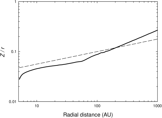
Finally, we compare our model values of with those predicted from detailed vertical structure models of irradiated accretion disks around T Tauri stars by D’Alessio et al. (1999). Their figure 1b (dashed curve) yields the following relation between the aspect ratio of the local scale height to radial distance and radial distance
| (A5) |
which is plotted by the dashed line in Figure 7. The solid line in Figure 7 shows our obtained aspect ratio for model 13 at t=0.3 Myr. It is evident that our is somewhat underestimated in the inner disk and overestimated in the outer disk but the disagreement between the two curves is within a factor of unity.
Appendix B Divergence of the viscous stress tensor
The components of in polar coordinates () are
| (B1) | |||||
| (B2) |
where we have neglected the contribution from off-diagonal components and . The components of the viscous stress tensor in polar coordinates () can be found in e.g. Vorobyov & Theis (2006).
References
- Adams et al. (1989) Adams, F. C., Ruden, S. P., & Shu F. H. 1989, ApJ, 347, 959
- André et al. (1993) André, P., Ward-Thompson, D., & Barsony, M. 1993, ApJ, 406, 122
- Andrews & Williams (2005) Andrews, S. M., & Williams, J. P. 2005, ApJ, 631, 1134
- Balbus & Hawley (1991) Balbus, S. A., & Hawley, J. F. 1991, ApJ, 376, 214
- Basu (1997) Basu, S. 1997, ApJ, 485, 240
- Boley et al. (2006) Boley, A. C., Mejía, A. C., Durisen, R. H., Cai, K., Pickett, M. K., DÁlessio, P. 2006, ApJ, 651, 517
- Boss (2008) Boss, A. 2008, ApJ, 677, 607
- Brown et al. (2000) Brown, D. W., et al. 2000, MNRAS, 319, 154
- Cai et al. (2008) Cai, K., Durisen, R. H., Boley, A. C., Pickett, M. K., Mejía, A. C. 2008, ApJ, 673, 1138
- Caselli et al. (2002) Caselli, P., Benson, P. J., Myers, P. C., & Tafalla, M. 2002, 572, 238
- D’Alessio et al. (1999) D’Alessio, P., Calvet, N., Hartmann, L., Lizano, S., & Cantó, J. 1999, ApJ, 527, 893
- Fukagawa et al. (2004) Fukagawa, M., et al. 2004, ApJ, 605, L53
- Grady et al. (1999) Grady, C. A., et al. 1999, ApJL, 523, L151
- Grady et al. (2001) Grady, C. A., et al. 2001, AJ, 122, 3396
- Hartmann et al. (1998) Hartmann, L., Calvet, N., Gullbring, E., & DÁlessio, P. 1998, ApJ, 495,385
- Hartmann et al. (2006) Hartmann, L., D’Alessio, P., Calvet, N., & Muzerolle, J. 2006, ApJ, 648, 484
- Johnson & Gammie (2003) Johnson, B. M., & Gammie C. F. 2003, ApJ, 597, 131
- Klessen (2001) Klessen, R. S. 2001, ApJ, 550, 77
- Kratter et al. (2008) Kratter, K. M., Matzner, Ch. D., Krumholz, M. R. 2008, ApJ, 681, 375
- Kroupa (2001) Kroupa, P. 2001, MNRAS, 322, 231
- Krumholz et al. (2007) Krumholz, M. R., Klein, R. I., & McKee, C. F. 2007, ApJ, 656, 959
- Lada (1987) Lada, Ch. J. 1987, in IAU Symp. 115, Star Forming Regions, editors M. Peimbert & J. Jugaku (Dordrecht: Reidel), p. 1
- Lada (2006) Lada, Ch. J. 2006, ApJL, 640, 63L
- Laughlin et al. (1997) Laughlin, G., Korchagin, V., & Adams, F. C. 1997, ApJ, 477, 410
- Laughlin et al. (1998) Laughlin, G., Korchagin, V., & Adams, F. C. 1998, ApJ, 504, 945
- Lodato & Rice (2004) Lodato, G., & Rice, W. K. M. 2004, MNRAS, 351, 630
- Lodato & Rice (2005) Lodato, G., & Rice, W. K. M. 2005, MNRAS, 358, 1489
- Looney et al. (2003) Looney, L. W., Mundy, L. G., & Welch, W. J. 2003, ApJ, 592, 255
- Lynden-Bell & Pringle (1974) Lynden-Bell, D., & Pringle, J. E. 1974, MNRAS, 168, 603
- Masunaga & Inutsuka (2000) Masunaga, H., & Inutsuka, S. 2000, ApJ, 531, 350
- Matzner & Levin (2005) Matzner, C. D., & Levin, Yu. 2005, ApJ, 628, 817
- Mayer et al. (2007) Mayer, L., Lufkin, G., Quinn, T., & Wadsley, J. 2007, ApJL, 661, 77
- Mejía (2004) Mejía, A. C. 2004, Ph.D. Dissertation, Indiana University
- Miller & Scalo (1979) Miller, G. E., & Scalo, J. M. 1979, ApJS, 41, 513
- Natta et al. (2001) Natta, A., Grinin, V. P., Mannings, V. 2001, in Protostars and Planets IV, ed. V. Mannings, A. P. Boss, S. S. Russell (Tucson: Univ. Arizona Press), 559
- Pickett et al. (2003) Pickett, B. K., Mejia, A. C., Durisen, R. H., Cassen, P. M., Berry, D. K., & Link R. P. 2003, ApJ, 590, 1060
- Rafikov (2005) Rafikov, R. R. 2005, ApJ, 621, 69
- Rice et al. (2003) Rice, W. K. M., Armitage, P. J., Bate, M. R., & Bonnell, I. A. 2003, MNRAS, 339, 1025
- Salpeter (1955) Salpeter, E. 1955, ApJ, 121, 161
- Shakura & Sunyaev (1973) Shakura, N. I., & Sunyaev, R. A. 1973, A&A, 24, 337
- Shu et al. (1990) Shu F. H., Tremaine S., Adams F.C., & Ruden S. P. 1990, ApJ, 358, 495
- Stamatellos et al. (2007a) Stamatellos, D., Hubber, D. A., & Whitworth, A. P. 2007, MNRAS, 382, L30
- Stamatellos et al. (2007b) Stamatellos, D., Whitworth, A. P., Bisbas, T., & Goodwin, S. 2007, A&A, 475, 37
- Stamatellos & Whitworth (2008) Stamatellos, D., & Whitworth, A. P. 2008, A&A, 480, 879
- Vorobyov & Basu (2005a) Vorobyov, E. I., & Basu, S. 2005, MNRAS, 360, 675
- Vorobyov & Basu (2005b) Vorobyov, E. I., & Basu, S. 2005, ApJL, 633, L137
- Vorobyov & Basu (2006) Vorobyov, E. I., & Basu, S. 2006, ApJ, 650, 956
- Vorobyov & Theis (2006) Vorobyov, E. I., & Theis, Ch. 2006, MNRAS, 373, 197
- Vorobyov & Basu (2007) Vorobyov, E. I., & Basu, S. 2007, MNRAS, 381, 1009
- Vorobyov & Basu (2008a) Vorobyov, E. I., & Basu, S. 2008a, ApJ, 676, 139
- Vorobyov & Basu (2008b) Vorobyov, E. I., & Basu, S. 2008b, submitted to MNRAS