Aging and effective temperatures near a critical point

Abstract

The orientation fluctuations of the director of a liquid crystal (LC) are measured after a quench near the Fréedericksz transition, which is a second order transition driven by an electric field. We report experimental evidence that, because of the critical slowing down, the LC presents several properties of an aging system after the quench, such as power law scaling in times of correlation and response functions. During this slow relaxation, a well defined effective temperature, much larger than the heat bath temperature, can be measured using the fluctuation dissipation relation.

The characterization of the thermodynamic properties of out of equilibrium and of slow relaxing systems is an important problem of great current interest, which is studied both theoretically and experimentally. In this framework an important and general question, which has been analyzed only theoretically is the relaxation of a system, which is rapidly quenched exactly at the critical point of a second order phase transition Peter ; Berthier ; Abriet2004 ; Gambassi ; Gambassi1 . Because of the well known divergence of the relaxation time and of the correlation length the system presents a very rich dynamic, which has been named “aging at the critical point”. Indeed this relaxation dynamic presents several properties, which are reminiscent of those observed during the aging of spin glasses Peter ; Berthier ; Gambassi ; Gambassi1 ; Abriet2004 ; Cugliandolo2002 ; Vincent : the mean quantity has an algebraic decay and the correlation and response functions exhibit a power law scaling in time. Another important feature analyzed during the aging at a critical point concerns the equilibrium relation between response and correlation, i.e. the fluctuation dissipation theorem (FDT), which is not necessarily satisfied in an out of equilibrium system. This statement is relevant in the context of spin glass aging where a well defined (in the thermodynamic sense) effective temperature $T_{\rm eff}$ can be obtained using the so called fluctuation dissipation relation (FDR). This relation leads to the introduction of the fluctuation dissipation ratio, $X$, between correlation and response functions Cugliandolo1997 ; Cugliandolo2002 . Deviations of $X$ from unity ($X=1$ is the equilibrium value) may quantify the distance from equilibrium Cugliandolo1997 . Equivalently an effective temperature $T_{\rm eff}=T/X$, larger than the heat bath temperature $T$, can be defined. Those ideas have been transferred to the aging at critical point, where for certain variables the FDR can be interpreted as a well defined effective temperature $T_{\rm eff}$ Peter ; Berthier .

The study of these analogies between the aging at the critical point and the aging of spin glasses is important because it allows to give new insight on the role of the quenched disorder on the above mentioned features and on the common mechanisms producing them. However these theoretical studies have been performed mainly on spin models and most importantly the reduced control parameter $\epsilon$ has been set exactly equal to zero. Thus one is interested to know how general these predictions are and also one may wonder whether those predictions can be observed in an experimental system where the exact condition $\epsilon=0$ can never be reached.

The purpose of this letter is to analyze, within this theoretical framework, an experiment on the relaxation dynamic close to the critical point of a liquid crystal instability, which is, at a first approximation, described by a Ginzburg-Landau equation and has the main features of a second order phase transition. The main result of our investigation is that after a quench close to the critical point the effective temperature $T_{\rm{eff}}$, measured from FDR, has a well defined value larger than the thermal bath temperature.

This kind of experimental test is important because the properties of $X$ and $T_{\rm eff}$ have attracted much interest, since they suggest that a generalized statistical mechanics can be defined for a broad class of non equilibrium phenomena. Several theoretical models or numerical simulations show such a behavior Cugliandolo2002 ; Berthier2007 . However in experiments the results are less clear and the relevance for real materials of the $T_{\rm{eff}}$ as defined by FDR is still an open question, which merits investigation Israeloff ; Bellon2001 ; Ocio ; Abou03 . For example, there are important differences, which are not understood, between supercooled fluids Israeloff , polymersBellon2001 , gelsAbou03 and spin glassesOcio . The point is that on this subject it is very difficult to find simple theoretical models, which can be directly compared with experiments. Thus the experimental study of the relaxation dynamics close to the critical point is very useful in this sense.

The system of our interest is the Fréedericksz transition of a liquid crystal (LC), subjected to an electric field $\vec{E}$ DeGennes ; Oswald . In this system, we measure the variable $\zeta$, which is the spatially averaged alignment of the LC molecules, whose local direction of alignment is defined by the unit pseudo vector $\vec{n}$. Let us first recall the general properties of the Fréedericksz transition. The system under consideration is a LC confined between two parallel glass plates at a distance $L=9$ $\mu$m. The inner surfaces of the confining plates have transparent Indium-Tin-Oxyde (ITO) electrodes, used to apply the electric field. Furthermore the plate surfaces, are coated by a thin layer of polymer mechanically rubbed in one direction. This surface treatment causes the alignment of the LC molecules in a unique direction parallel to the surface (planar alignment),i.e. all the molecules have the same director parallel to the $x$-axiscell . The cell is next filled by a LC having a positive dielectric anisotropy (p-pentyl-cyanobiphenyl, 5CB, produced by Merck). The LC is subjected to an electric field perpendicular to the plates, by applying a voltage $V$ between the ITO electrodes, i.e. ${E}=V/L$. To avoid the electrical polarization of the LC, we apply an AC voltage at a frequency $f_{V}=1$ kHz ($V=\sqrt{2}V_{0}\cos(2\pi f_{V}t)$) DeGennes ; Oswald . More details on the experimental set-up can be found in ref.Joubaud_upon ; joubaud2008 . When $V_{0}$ exceeds a threshold value $V_{c}$ the planar state becomes unstable and the LC molecules, except those anchored to the glass surfaces, try to align parallel to the field, i.e. the director, away from the confining plates, acquires a component parallel to the applied electric field ($z$-axis). This is the Fréedericksz transition whose properties are those of a second order phase transition DeGennes ; Oswald . For $V_{0}$ close to $V_{c}$ the motion of the director is characterized by its angular displacement $\theta$ in $xz$-plane ($\theta$ is the angle between the $x$ axis and $\vec{n}$), whose space-time dependence has the following form : $\theta=\theta_{0}(x,y,t)\sin\left(\frac{\pi z}{L}\right)$ DeGennes ; Oswald ; SanMiguel1985 . If $\theta_{0}$ remains small then its dynamics, neglecting the $(x,y)$ dependence of $\theta_{0}$, is described by a Ginzburg-Landau equation :

$$\tau_{0}\frac{{\rm d}\theta_{0}}{{\rm d}t}=\epsilon\ \theta_{0}-{1\over 2}(\kappa+\epsilon+1)\theta_{0}^{3}+\eta$$ (1)

where $\epsilon=\frac{V_{0}^{2}}{V_{c}^{2}}-1$ is the reduced control parameter. The characteristic time $\tau_{0}$ and constant $k$ depend on the LC material properties. $\eta$ is a thermal noise delta-correlated in time SanMiguel1985 .

We define the variable $\zeta$ as the spatially averaged alignment of the LC molecules and more precisely :

$$\zeta=\frac{2}{L}\frac{1}{\mathcal{A}}\int\int_{\mathcal{A}}\mathrm{d}x\mathrm{d}y\int_{0}^{L}(1-n_{x}^{2})\mathrm{d}z$$ (2)

where $\mathcal{A}=\pi D_{0}^{2}/4$ is the area, in the ($x$, $y$) plane, of the measuring region of diameter $D_{0}$, which is about $2$ mm in our case. If $\theta_{0}$ remains small, $\zeta$ takes a simple form in terms of $\theta_{0}$, i.e. $n_{x}=\cos(\theta)$ and $\ \zeta=1/\mathcal{A}\int\int_{\mathcal{A}}\mathrm{d}x\mathrm{d}y\theta_{0}^{2}$. It has been shown that $\zeta$ is characterized by a mean value $\langle\zeta\rangle\propto\epsilon$, by a divergent relaxation time $\tau=\tau_{o}/\epsilon$ and by fluctuations, which have a Lorentzian spectrum Galatola ; joubaud2008 . The measure of the variable $\zeta$ relies upon the anisotropic properties of the LC, i.e. the cell is a birefringent plate whose local optical axis is parallel to $\vec{n}$. This optical anisotropy can be precisely measured using a polarization interferometer Bellon02 , which has a signal to noise ratio larger than 1000 (see ref. Joubaud_upon ; joubaud2008 for details).

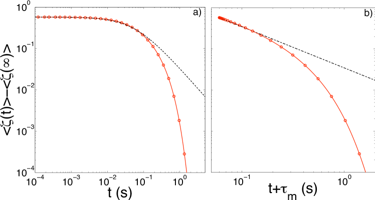
Figure 1: a) Mean relaxation of the system, $\log\langle\zeta(t)\rangle$, as a function of time after a quench ($\circ$) from $\epsilon_{1}=0.3$ to $\epsilon_{0}=0.01$. The continuous line represents the theoretical response based on eq. 1 with $\langle\zeta\rangle\simeq\psi_{0}^{2}$. b) Mean relaxation of the system as a function of the reduced time $(t+\tau_{m})$. in both figures the dashed lines represents the theoretical relaxation at $\epsilon=0$.

In this letter, we consider the dynamics of $\zeta$ as a function of time after a quench from $\epsilon=\epsilon_{1}>0.3$ to $\epsilon=\epsilon_{0}<<0.1$. The fact that the control parameter is the electric field allows one to have extremely fast quenches, typically $1$ ms. As the typical relaxation time $\tau$ of $\zeta$ is about $10s$, at $\epsilon_{0}\simeq 0$, this means that we can follow the out of equilibrium dynamics for about four orders of magnitude in time, which is really comparable to what is done in real glass experiments after a temperature quench, where the dynamics is usually followed for about 3 or 4 decades in time. The advantage here is that this relaxation dynamics, which lasts only a few seconds, allows us to repeat the experiment several times and to perform an ensemble average (indicated by $<\cdot>$) of the measured quantities. We consider first the specific case of a quench from $\epsilon_{1}=0.3$ to $\epsilon_{0}=0.01$. The typical mean value $<\zeta(t)>$ of $\zeta$ after this quench is plotted in fig. 1 as a function of time $t$ ($t=0$ is the time when the quench has been performed). This mean dynamics of $\zeta$ is obtained by repeating the same quench $7000$ times. The behavior of $<\zeta>$ remains constant for a certain time and then slowly relaxes (see fig. 1a). Above a characteristic time, which is about $0.22$ s in our case, the relaxation becomes exponential.

To understand this behavior, we decompose the dynamics of $\theta_{0}$ in a mean dynamics after the quench and its fluctuations, i.e. $\theta_{0}=\psi_{0}(t)+\delta\theta_{0}$, where $\psi_{0}(t)=\langle\theta_{0}(t)\rangle$. The dynamics of $\Psi_{0}$ obtained from the analytical solution of eq.1 is shown in fig.1 as a continuous line, which perfectly agrees with the measured dynamics. The experimental data and the solution of eq.1 have two well distinguish limits : for $t\gg\tau\equiv\tau_{0}/(2\epsilon)$, the relaxation is exponential ($\tau\simeq 0.22s$ at $\epsilon_{0}=0.01$) ; for $t\ll\tau\equiv\tau_{0}/(2\epsilon_{0})$, the dynamics of $\psi_{0}$ is almost algebraic : $\psi_{0}(t)=\left[{(\kappa+1)\over\tau_{0}}\left(t+\tau_{m}\right)\right]^{-1/2}$ with $\tau_{m}=\frac{\tau_{0}}{(\kappa+1)\psi_{0}(0)^{2}}$. This behavior, plotted in fig. 1 as a dashed line, is identical to the relaxation at the critical point Gambassi . Thus the system should present aging phenomena in the range $t<\tau$, which is the interval where the dashed line follows the experimental data in fig. 1.

In order to measure $T_{\rm eff}$ as defined by the FDR, we need to measure both the correlation function $C_{\theta}(t,t_{w})\equiv\langle\ \delta\theta_{0}(t)\ \delta\theta_{0}(t_{w})\rangle$ of the thermal fluctuations $\delta\theta_{0}$ of $\theta_{0}$ and the response function $\chi(t,t_{w})$ of $\theta_{0}$, at time $t$ to a perturbation, given at time $t_{w}$, to its conjugated variable $\Gamma$, with $t_{w}<t$. More precisely, from ref.Cugliandolo1997 ; Cugliandolo2002 the effective temperature is given by:

$$\chi(t,t_{w})={X(t,t_{w})\over k_{B}T}[C_{\theta}(t,t)-C_{\theta}(t,t_{w})]$$ (3)

where $k_{B}$ is the Boltzmann constant,T the heat bath temperature, i.e. $T_{\rm eff}=T/X(t,t_{w})$.

To compute $\chi(t,t_{w})$ and $C_{\theta}(t,t_{w})$ in our experiment one has to consider that the measured variable is $\zeta$. The relationship between the fluctuations of $\zeta$ and $\theta_{0}$ has been discussed in details in ref.Joubaud_upon , thus we recall here only the useful results. As the area of the measuring beam is much larger than the correlation length, the global variable measured by the interferometer is $\zeta=\frac{1}{\mathcal{A}}\iint\theta_{0}^{2}\mathrm{d}x\mathrm{d}y\simeq\psi_{0}^{2}+2\psi_{0}\delta\theta_{0}$. Thus the mean value of $\zeta$ is $\langle\zeta(t)\rangle=\psi_{0}^{2}(t)$ and the fluctuations of $\delta\zeta$ of $\zeta$ can be related to the fluctuations of $\theta_{0}$ : $\delta\zeta(t)=2\psi_{0}(t)\delta\theta_{0}(t)$.

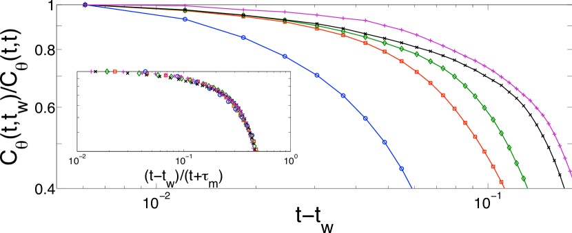
Figure 2: a) Correlations functions $C_{\theta}(t,t_{w})$ as a function of $t-t_{w}$ for different fixed $t=0.06\ s$ ($\circ$), $0.2\ s$ ($\Box$), $0.26\ s$ ($\diamond$), $0.28\ s$ ($\times$) and $0.31\ s$ ($+$) after the same quench of fig. 1. Inset: The correlation functions have a simple master curve obtained by plotting $C_{\theta}(t,t_{w})/C_{\theta}(t,t_{w})$ versus $(t-t_{w})/(t+\tau_{m})$. Notice that $(t+\tau_{m})$ is the reduced time used in fig.1

The autocorrelation function of $\theta_{0}$ is obtained using the values of $\psi_{0}(t)$ and $\psi_{0}(t_{w})$, i.e. $C_{\theta}(t,t_{w})=\langle\zeta(t)\zeta(t_{w})\rangle/(4\psi_{0}(t)\psi_{0}(t_{w}))$. The $C_{\theta}(t,t_{w})$, measured at various fixed $t$, are plotted as function of $t-t_{w}$ in fig.2. We see that a simple scaling of the correlation function can be obtained by plotting them as a function of $(t-t_{w})/(t+\tau_{m})$. Thus in agreement with theoretical predictions, our system presents, during its slow relaxation after the quench close to the critical point, algebraic decay of mean quantities and the scaling of correlation functions, which are very similar to the main features of spin glass aging (see for example Cugliandolo2002 ; Vincent ).

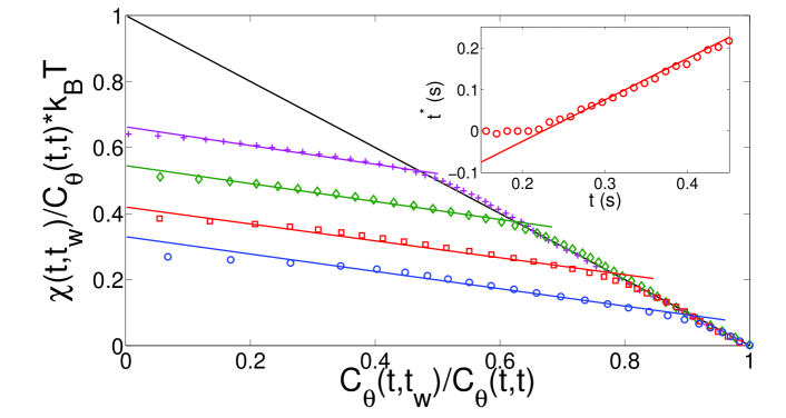
Figure 3: a) Parametric plot of integrated response versus correlation for $t=0.4$ s ($\circ$), $0.5$ s ($\Box$), $0.6$ s ($\diamond$) and $0.7$ s ($+$). Continuous line are linear fits. Dark line represents the FDT at equilibrium. Inset : the characteristic time $t^{*}$ is plotted as a function of $t$.

The response function is obtained by applying a small change of the voltage $V_{0}$, which modifies the control parameter, i.e. $\epsilon=\epsilon_{0}+\delta\epsilon$. In ref.Joubaud_upon we have shown that the external torque $\Gamma_{ext}$, i.e. the conjugated variable of $\theta_{0}$, associated to $\delta\epsilon$ is equal to :

$$\Gamma_{\rm ext}=2B\ \delta\epsilon\ \psi_{0}(t)\ \left(1-\frac{\psi_{0}(t)^{2}}{2}\right)$$ (4)

We separate $\theta_{0}(t)$ into the average part $\psi_{0}(t)$, solution of eq. 1, with $\eta=0$, and a deviation $\Delta(t)$ due to $\delta\epsilon$ : $\theta_{0}(t)=\psi_{0}(t)+\Delta(t)$. We define the linear response function $R(t,t_{w})=<\Delta>/\Gamma_{\rm ext}$ of $\theta_{0}$ to $\Gamma_{ext}$ using a Dirac delta function for $\delta\epsilon$ at an instant $t_{w}$, i.e. $\delta\epsilon(t)\propto\delta(t-t_{w})$. In the experiment the Dirac delta function is approximated by a triangular function of amplitude $\delta\epsilon_{0}$ and duration $\tau_{r}\simeq 2ms<<\tau$, specifically: $\delta\epsilon=\delta\epsilon_{0}(1-2|t-t_{w}|/\tau_{r}$ for $|t-t_{w}|<\tau_{r}/2$ and $\delta\epsilon=0$ for $|t-t_{w}|>\tau_{r}/2$, with $\tau_{r}/\tau\simeq 10^{-4}$. The measured quantity is the response $R_{\zeta,\delta\epsilon}=<\Delta\zeta>/\delta\epsilon$, of $\zeta(t)$ to $\delta\epsilon(t_{w})$. As $\Delta\zeta(t)=2\psi_{0}(t)\Delta$ it follows that the linear response of $\theta_{0}$ to $\Gamma_{ext}$ is:

$$R(t,t_{w})=\frac{R_{\zeta,\delta\epsilon}(t,t_{w})}{4B\ \psi_{0}(t_{w})\ \psi_{0}(t)\ \left(1-\frac{\psi_{0}(t_{w})^{2}}{2}\right)}$$ (5)

where $B=A\pi^{2}K_{1}/(4L)$, and $K_{1}$ a LC elastic constant. Thus inserting in eq.5 the measured values of $R_{\zeta,\delta\epsilon}(t,t_{w})$, of $\psi_{0}(t)$ and of $\psi_{0}(t_{w})$ we can measure $R(t,t_{w})$ and by numerical integration we finally obtain $\chi(t,t_{w})=\int_{t}^{t_{w}}R(t,t^{\prime})\mathrm{d}t^{\prime}$. The accuracy of this procedure has been checked at equilibrium in ref.Joubaud_upon , where we have shown that the measured $C_{\theta_{0}}$ and $\chi(t,t_{w})$ verify FDT.

The integrated response is related to the correlation by the FDR relations (see eq. 3). Due to the non-equilibrium process, it is not equivalent whether the parameter is the waiting time $t_{w}$ or the observation time $t$ (see ref.Berthier2007 for a detailed discussion on this point). Applying the correct procedure Cugliandolo1997 ; Berthier , we keep the time $t$ constant and we vary $t_{w}$, i.e. $0<t_{w}<t$, and we repeat the procedure at various $t$. Following ref.Cugliandolo1997 , we study the FDR during the relaxation process by plotting the integrated response $\chi$ as a function of $C_{\theta}$. These FDR plots can be seen in fig. 3 for four characteristic values of $t$. When the system is in equilibrium the FDR plot is a straight line with slope $-1/(k_{B}T)$ (continuous line in fig. 3). The curves in fig. 3 for each $t$ are composed by two straight lines and are remarkably similar to those predicted in theoretical models Cugliandolo1997 and seen in experiments Ocio of spin glasses aging. When $t_{w}$ is close to $t$, i.e. large values of $C(t,t_{w})$, the FDT is satisfied, i.e. the experimental points are on the continuous line in fig. 3. For $C(t,t_{w})$ smaller than a value $C^{*}$, which depends on $t$, the FDT is not satisfied. However $\chi(t,t_{w})$ remains linear in $C(t,t_{w})$ but the slope, which does not depend on $t$, is much smaller than its value at equilibrium. This means that the slow modes of the systems have a very well defined $T_{eff}$, independent of $t$, higher than the temperature of the bath. Precisely we find, for $C(t,t_{w})<C^{*}$, $X=T/T_{\rm eff}=0.31$, which is remarkably close to the asymptotic value $X=0.305$ analytically Gambassi1 and numerically Berthier estimated for the small wave vector modes of an Ising model quenched at the critical point using a different quenching procedure. This analogy is important because our measurement, being an integral over the measuring volume, is more sensitive to the fluctuations of the long wavelength modes. In fig.3 we see that $C^{*}$ is a decreasing function of $t$. Let us define $t^{*}$ as the characteristic time associated with $C^{*}$. In the inset of fig. 3, we have plotted the value of $t^{*}$ as a function of $t$. We find that $t^{*}\simeq 0$ for $t\leq\tau=0.22s$. This indicates that, in agreement with ref.Berthier ; Gambassi ; Gambassi1 , the violation occurs for all times at $\epsilon_{0}=0$. In our case it is cut by the exponential relaxation, which starts at $t\simeq\tau$. For $t>\tau$, $t^{*}=t-\tau$ is linear in $t$, which also agrees with the theoretical picture of the FDR Cugliandolo1997 . Indeed $t^{*}$ separates the equilibrium part and the aging one and the ratio $t^{*}/t=1-\tau/t$, for $t>\tau$, defines how large is the equilibrium interval with respect to the total time. Notice that at $\epsilon_{0}=0$, $\tau=\infty$ and the equilibrium interval does not exist Berthier . Thus the values of $\epsilon_{0}$ and $\epsilon_{1}$ affect only the amplitude of the region where the out of equilibrium is observed but not the value of $X$long . We also want to stress that this very clear scenario, with a well defined $T_{\rm eff}$ independent of $t$, is obtained only if the right procedure with fixed $t$ is used Berthier ; Berthier2007 . The results are completely different if $t_{w}$ is kept fixed. In such a case $T_{\rm eff}$ is a decreasing function of $t_{w}$ long . The non-commutability of the two procedures, i.e. either with $t$ or with $t_{w}$ fixed, shows the non ergodicity of the phenomenon and opens a wide discussion on how to analyze the data in more complex situations, such as those where $T_{eff}$ is measured in real materials and the procedure with $t_{w}$ fixed is often used Israeloff ; Bellon2001 ; Ocio ; Abou03 .

In conclusion we have shown that a LC quenched close to the critical point of the Fréedericksz transition presents aging features, such as a power law scaling of correlation functions and the appearance of a well defined $T_{\rm{eff}}>T$. Most importantly we show the existence of a well defined $T_{\rm eff}$ if the the right procedure with fixed $t$ is used. What is very interesting here is that although we are not exactly at $\epsilon_{0}=0$ we observe a large interval of time,$0<t<\tau$ where the predicted aging at critical point can be observed. The results plotted in fig.3 agree with those of ref. Berthier ; Gambassi1 but are different from those predicted for mean-field Gambassi . This opens the discussion for further theoretical and experimental developments. It also shows that the study of the quench at critical point is an interesting and not completely understood problem by itself Berthier ; Gambassi .

We acknowledge useful discussion with P. Holdsworth, L. Berthier, M. Henkel and M. Pleimling . This work has been partially supported by ANR-05-BLAN-0105-01.

References

- (1) L. Berthier, P.C.W. Holdsworth and M. Sellitto, J. Phys. A: Math. Gen., 34, pp.1805 – 1824 (2001)
- (2) P. Mayer, L. Berthier, J. P. Garrahan, P. Sollich, Phys. Rev. E, 68, 016116 (2003)
- (3) S. Abriet, D. Karevski, E.P.J. B, 37(1), 47-53 (2004)
- (4) P. Calabrese, A. Gambassi and F. Krzakala, J. Stat. Mech. : Theory and Experiment, P06016 (2006)
- (5) P. Calabrese and A. Gambassi, Phys. Rev. E 66, 066101 (2002).
- (6) L. Cugliandolo,Dynamics of glassy systems, Lecture notes (Les Houches, July 2002),[cond-mat/0210312]
- (7) E. Vincent, in Ageing and the Glass Transition edited by M. Henkel, M. Pleimling, R. Sanctuary (Springer-Verlag, Berlin 2007).
- (8) L. Cugliandolo, J. Kurchan and L. Peliti, Phys. Rev. E, 55(4) 3898 (1997)
- (9) L. Berthier,Phys. Rev. Lett., 98, 220601 (2007)
- (10) T.S. Grigera and N.E. Israeloff, Phys. Rev. Lett., 83, 5038(1999)
- (11) B. Abou and F. Gallet, Phys. Rev. Lett. 93, 160306 (2003); S. Jabbari-Farouji, et al. Phys. Rev. Lett. 98, 108302 (2007); S. Jabbari-Farouji, et. al. arXiv:0804.3387v1.; N. Greinert, T. Wood, and P. Bartlett, Phys. Rev. Lett. 97, 265702 (2006); P. Jop, A. Petrosyan, and C. Ciliberto, Phyl. Magazine,88, 33, 4205 (2008).
- (12) L. Bellon, S. Ciliberto, C. Laroche Europhys. Lett., 53(4), 511 (2001); L. Buisson and S. Ciliberto Physica D, 204(1-2) 1 (2005)
- (13) D. Hérisson and M. Ocio, Phys. Rev. Lett., 88(25), 257202 (2002)
- (14) P.G. de Gennes and J. Prost,The physics of liquid crystals(Clarendon Press, Oxford, 1993)
- (15) P. Oswald and P. Pieranski, Nematic and cholesteric liquid crystals (Taylor & Francis, Boca Raton, 2005)
- (16) To check for anchoring and pretilt effects, several kind of coatings (commercial and home-made) have been used. The results are independent on the type of coating used.
- (17) S. Joubaud, G. Huilard, A. Petrosyan and S. Ciliberto, J. Stat. Mech., P01033, (2009). (arXiv:0810.1448)
- (18) S. Joubaud, A. Petrosyan, S.Ciliberto, N. Garnier, 2008 Phys. Rev. Lett. 100 180601
- (19) M. San Miguel, Phys. Rev. A 32(6) 3811 (2005)
- (20) L. Bellon, S. Ciliberto, H. Boubaker, L. Guyon, Optics Communications 207 49 (2002).
- (21) P. Galatola and M. Rajteri, Phys. Rev. 49, 623 (1994)
- (22) More details on this point will be given in a longer report.