Saturation of Two Level Systems and Charge Noise in Josephson Junction Qubits

Abstract

We study the charge noise $S_{Q}$ in Josephson qubits produced by fluctuating two level systems (TLS) with electric dipole moments in the substrate. The TLS are driven by an alternating electric field of angular frequency $\Omega$ and electric field intensity $I$. It is not widely appreciated that TLS in small qubits can easily be strongly saturated if $I\gg I_{c}$, where $I_{c}$ is the critical electric field intensity. To investigate the effect of saturation on the charge noise, we express the noise spectral density in terms of density matrix elements. To determine the dependence of the density matrix elements on the ratio $I/I_{c}$, we find the steady state solution for the density matrix using the Bloch-Redfield differential equations. We then obtain an expression for the spectral density of charge fluctuations as a function of frequency $f$ and the ratio $I/I_{c}$. We find $1/f$ charge noise at low frequencies, and that the charge noise is white (constant) at high frequencies. Using a flat density of states, we find that TLS saturation has no effect on the charge noise at either high or low frequencies.

I Introduction

The superconducting Josephson junction qubit is a leading candidate in the design of a quantum computer, with several experiments demonstrating single qubit preparation, manipulation, and measurement, Vion et al. (2002); Yu et al. (2002); Martinis et al. (2002); Chiorescu et al. (2003) as well as the coupling of qubits. Pashkin et al. (2003); Berkley et al. (2003) A significant advantage of this approach is scalability, as these qubits may be readily fabricated in large numbers using integrated circuit technology. However, noise and decoherence are major obstacles to using superconducting Josephson junction qubits to construct quantum computers. Recent experiments Simmonds et al. (2004); Martinis et al. (2005) indicate that a dominant source of decoherence is two level systems (TLS) that are fluctuating in the insulating barrier of the tunnel junction as well as in the dielectric material used to fabricate the circuit, e.g., the substrate. The two level fluctuators that have electric dipole moments can induce image charges in the nearby superconductor and hence produce charge noise $S_{Q}(\omega)$. Zimmerli et al. (1992); Visscher et al. (1995); Zorin et al. (1996); Kenyon et al. (2000); Astafiev et al. (2006); Shnirman et al. (2005); Faoro et al. (2005); Faoro and Ioffe (2006)

Previous theories of charge noiseShnirman et al. (2005); Faoro et al. (2005); Faoro and Ioffe (2006) have neglected the important issue of the saturation of the two level systems by electric fields used to manipulate the qubits. Dielectric (ultrasonic) experiments on insulating glasses at low temperatures have found that when the electric (acoustic) field intensity $I$ used to make the measurements exceeds the critical intensity $I_{c}$, the dielectric (ultrasonic) power absorption by the TLS is saturated, and the attenuation decreases as the field intensity increases. Hunklinger and Arnold (1976); Golding et al. (1976); Graebner et al. (1983); Schickfus and Hunklinger (1977); Martinis et al. (2005) (If ${\cal{E}}\cos(\Omega t)$ denotes the electric field, then we define the intensity $I={\cal{E}}^{2}$.) Previous theories of charge noise in Josephson junctions assumed that the TLS were not saturated, i.e., that $I\ll I_{c}$. This seems sensible since charge noise experiments Astafiev et al. (2004) have been done in the limit where the qubit absorbed only one photon.

However, the following simple estimate shows that stray electric fields associated with this photon could saturate two level systems in the dielectric substrate which supports the qubit. We can estimate the voltage $V$ across the capacitor associated with the substrate and ground plane beneath a Cooper pair box (see Fig. 1) by setting $CV^{2}/2=\hbar\omega$ where $\hbar\omega$ is the energy of the microwave photon. We estimate the capacitance $C=\varepsilon_{o}\varepsilon_{r}A/L\sim 7$ aF using the area $A=40\times 800$ nm² of the Cooper pair box, the thickness $L=400$ nm of the substrate,Astafiev et al. (2004) and the relative permittivity $\varepsilon_{r}=10$. Using $\omega/2\pi=f=10$ GHz, we obtain a voltage of $V\sim 1.4\;$mV. A substrate thickness $L$ of 400 nm yields an electric field of ${\cal{E}}\sim 3.4\times 10^{3}$ V/m.

We can compare this with the critical intensity $I_{c}$ and the associated critical electric field ${\cal{E}}_{c}$ which has been measured experimentally Martinis et al. (2005). Martinis et al. Martinis et al. (2005) measured the low temperature dielectric loss tangent of amorphous SiO₂ at $f=7.2$ GHz and amorphous SiN_x at $f=4.7$ GHz as a function of the root-mean-square (rms) voltage. They found that the loss tangent was constant at low power, but rolled over and decreased above a critical rms voltage $V_{c}\sim 0.2\;\mu$V. For a capacitor thickness of 300 nm, the associated critical field is ${\cal{E}}_{c}\sim 0.7$ V/m. So ${\cal{E}}/{\cal{E}}_{c}\sim 5\times 10^{3}$, and $I/I_{c}=\left({\cal{E}}/{\cal{E}}_{c}\right)^{2}\sim 2\times 10^{7}\gg 1$.

We can do a similar estimate to show that a single photon would even more strongly saturate resonant TLS in the insulating barrier of the tunnel junction. We use the same numbers as before but with $C=1$ fF and the thickness of the junction $L=1.5$ nm to obtain ${\cal{E}}\sim 7\times 10^{4}$ V, and $I/I_{c}\sim 10^{10}\gg 1$.

However, there are only a few TLS in the oxide barrier of a small tunnel junction as the following estimate shows. For a parallel plate capacitor with $L=1.5$ nm and $A=1\;\mu$m², the volume is $V_{o}=1.5\times 10^{-21}$ m³. The typical TLS density of states Phillips (1981) is $10^{46}/Jm^{3}$. However, only a fraction of these have electric dipole moments. So we will assume that the density of states of TLS with electric dipole moments is $P_{TLS}\simeq 10^{45}/Jm^{3}\simeq 663/h$GHz$\mu$m³. Using this value of $P_{TLS}$, we find that in a small tunnel junction, there are only 2 TLS with an energy splitting less than 10 GHz. A single fluctuator would have a Lorentzian noise spectrum. The presence of $1/f$ noise implies many more than 2 fluctuators. It is likely that these additional fluctuators are in the substrate. Our main point is that TLS in small devices are easily saturated. It is therefore important to analyze the effect of TLS saturation on the charge noise both at low and high frequencies $f$ of the noise spectrum.

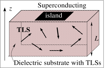
Figure 1: (Color online) Distribution of two level systems (TLS) in the dielectric substrate of a Cooper pair box. The superconducting island with the Josephson junction qubit is the black rectangle on the top of the substrate. There is a ground plane underneath the substrate.

In this article, we explore the consequences of this saturation on the spectral density of polarization and charge fluctuations. We consider a driven system consisting of two level systems with electric dipole moments that fluctuate randomly, leading to fluctuations $\delta P(t)$ in the polarization denoted by $P(t)$. In addition, the dipole moments of these TLS couple to an applied ac electric field that drives the system with an angular frequency $\Omega$.

Let us consider a single two level system. According to the Wiener-Khintchine theorem, in the stationary state the polarization noise spectral density $S_{P}(\omega)$ of this two level system is twice the Fourier transform of the polarization autocorrelation function:

$$S_{P}(\omega) = 2\int_{-\infty}^{+\infty}\mbox{d}(t_{1}-t_{2})\mbox{e}^{i\omega(t_{1}-t_{2})}\left[\langle\delta P(t_{1})\delta P(t_{2})\rangle\right]_{\rho}$$

$$= 2\int_{-\infty}^{+\infty}\mbox{d}(t_{1}-t_{2})\mbox{e}^{i\omega(t_{1}-t_{2})}\mbox{Tr}\{\rho\langle\delta P(t_{1})\delta P(t_{2})\rangle\}$$

where $[...]_{\rho}$ denotes a trace over the density matrix $\rho$, and $\langle...\rangle$ denotes an average over the time series. $\delta P(t)=[P(t)-\langle P\rangle]$ is the fluctuation in the polarization $P(t)$ at time $t$ and $\langle P\rangle$ is the polarization averaged over the time series. From the convolution theorem, $S_{P}(\omega)\sim|\delta P(\omega)|^{2}$. If the average over the density matrix is equivalent to an average over the time series, then one can easily show that $\delta P(\omega=0)=0$ and hence, $S_{P}(\omega=0)=0$.

We assume that the total density matrix $\rho_{T}$ is the product of two factors: one factor $\rho$ that contains the contributions of the ac driving field and the other that contains the contributions of the random fluctuations of the dipoles. We make this division because we can find the time dependence of the density matrix (in the Schroedinger representation) due to the driving field by solving the Bloch-Redfield equations. Since it is not clear how to include the random fluctuations of the two level systems in the Hamiltonian and hence, in the Bloch-Redfield equations, we will treat the random fluctuations separately. So the density matrix $\rho$ contains the contributions of the driving field to $S_{P}(\omega)$ while the polarization autocorrelation function $\langle\delta P(t_{1})\delta P(t_{2})\rangle$ contains the contributions of the random fluctuations of the electric dipoles. We will solve the Bloch-Redfield equations in steady state to find the time evolution of the density matrix $\rho(t)$ and its dependence on the ratio $I/I_{c}(\Omega,T)$ of the electric field intensity $I$ to the critical intensity $I_{c}(\Omega,T)$ which is a function of the driving angular frequency $\Omega$ and the temperature $T$. The benefit of this approach is that it is valid in both equilibrium as well as steady state non-equilibrium situations. From the polarization noise spectral density, we can obtain the charge noise $S_{Q}(\omega)$. We then average over the distribution of independent TLS. Unlike previous theoretical efforts,Shnirman et al. (2005); Faoro et al. (2005); Faoro and Ioffe (2006) we use the standard TLS density of states that is a constant independent of energy.

At low frequencies ($hf\ll k_{B}T$) the system is in equilibrium, and we find $1/f$ charge noise that is proportional to the temperature and to the dielectric loss tangent $\tan\delta$ that has a well known contribution from the electric dipole moments of TLS.Phillips (1981); Classen et al. (1994); Hunklinger and Arnold (1976) In addition the low frequency charge noise has negligible dependence on the electric field intensity ratio $I/I_{c}$.

At high frequencies ($hf\gg k_{B}T$) we find that the charge noise is white noise independent of frequency. It has a very weak dependence on the ratio $I/I_{c}(\Omega,T)$ and the driving frequency $\Omega$. We also find that the amplitude of the high frequency white charge noise decreases gradually as the temperature increases. The fact that the charge noise spectrum depends very weakly on the ratio $I/I_{c}(\Omega,T)$ indicates that the saturation of two level systems does not affect charge noise.

The paper is organized as follows. In Section II, we present our model of a TLS in an external driving field. In Section III, we use the fluctuation-dissipation theorem to give an expression for the charge noise in thermal equilibrium. In Section IV, we take a more general approach that is valid in both equilibrium and nonequilibrium cases. In particular, we derive a general analytic expression for the spectral density of polarization and charge fluctuations of an individual two level system (also referred to as a fluctuator) in terms of the density matrix. In Section V, we solve the Bloch-Redfield linear differential equations for the density matrix. We find the steady state solution of the Bloch-Redfield equations and we analyze its dependence on the ratio $I/I_{c}(\Omega,T)$. In Section VI, we investigate the noise spectrum of a single random telegraph fluctuator. We then average over the distribution of independent TLS numerically to determine the frequency dependence of the noise spectrum. A summary is given in Section VII.

II Two Level System (TLS)

In applying the standard model of two level systems to Josephson junction devices, we consider a TLS that sits in the insulating substrate or in the tunnel barrier, and has an electric dipole moment ${\bf p}$ consisting of a pair of opposite charges separated by a distance $d$. The electrodes positioned at $z=0$ and $z=L$ are kept at the same potential. The angle between ${\bf p}$ and the $z$–axis, perpendicular to the electrodes, is $\theta$. The dipole induces charge on the electrodes. As we show in the appendix, the magnitude of the induced charge $Q$ on each electrode is proportional to the $z$-component of the dipole moment, $p_{z}=p\cos\theta$, i.e.,

$$Q=\left|\frac{p\cos\theta}{L}\right|$$ (1)

The dipole flips and induces polarization fluctuations and hence charge fluctuations on the electrodes.

The TLS is in a double–well potential with a tunneling matrix element $\Delta_{0}$ and an asymmetry energy $\Delta$.Phillips (1981) The Hamiltonian of a TLS in an external ac field can be written as $H(t)=H_{0}+H_{1}(t)$, where $H_{0}=\frac{1}{2}(\Delta\sigma_{z}+\Delta_{0}\sigma_{x})$, and $H_{1}(t)=-\sigma_{z}{\bf p}\cdot\bm{\xi}_{ac}(t)$. Here $\sigma_{x,z}$ are the Pauli spin matrices and $\bm{\xi}_{ac}(t)=\bm{\xi}_{ac}\cos\Omega t$ is a small perturbing ac electric field of angular frequency $\Omega$ that couples to the TLS electric dipole moment. $\bm{\xi}_{ac}$ points along the $z-$axis.

After diagonalization of $H_{0}$, the Hamiltonian becomes

$$H(t) =H_{0}+H_{1}(t)$$ (2)

$$H_{0} =\frac{1}{2}E\sigma_{z}$$ (3)

$$H_{1}(t) =-\eta(\Delta_{0}\sigma_{x}+\Delta\sigma_{z})\mbox{cos}\Omega t,$$ (4)

where $E=\sqrt{\Delta^{2}+\Delta_{o}^{2}}$ is the TLS energy splitting and $\eta\equiv{\bf p}\cdot\bm{\xi}_{ac}/E$. Notice that $\eta$ is a small dimensionless variable ($\eta\approx 5\times 10^{-3}$ for $p=3.7$ D, $\xi_{ac}\approx 10^{3}$ V/m and $E/h\approx 10$ GHz). (The dipole moment of an OH^- molecule is 3.7 D.Golding et al. (1979)) The energy eigenbasis is denoted by $\{|+\rangle,|-\rangle\}$, and the corresponding eigenvalues are $E_{\pm}=\pm E/2$, where $+$ $(-)$ refers to the upper (lower) level of the TLS. The energy splitting $E$ will also be referred to as $\hbar\omega_{0}$.

An excited two level system can decay to the ground state by emitting a phonon. The longitudinal relaxation rate is given by:Phillips (1981)

$$T_{1}^{-1}=\frac{\gamma_{d}^{2}}{\left(2\pi\rho\hbar^{4}\right)}\left[\left(\frac{1}{c_{\ell}^{5}}\right)+\left(\frac{2}{c_{t}^{5}}\right)\right]E\Delta_{o}^{2}\coth\left(\frac{E}{2k_{B}T}\right)~{},$$ (5)

where $\rho$ is the mass density, $c_{\ell}$ is the longitudinal speed of sound, $c_{t}$ is the transverse speed of sound, and $\gamma_{d}$ is the deformation potential. In this paper we will use the values for SiO₂: $\gamma_{d}=$1 eV, $\rho=$ 2200 kg/m³, $c_{\ell}$=5800 m/s, and $c_{t}$=3800 m/s. Typically, $T_{1}$ varies between $10^{-9}$ s and $10^{4}$ s for temperatures around 0.1 K. The distribution of TLS parameters is given by Phillips (1987, 1981)

$$P(E,T_{1})=\frac{P_{TLS}}{2T_{1}\sqrt{1-\left(\tau_{min}(E)/T_{1}\right)}},$$ (6)

where $P_{TLS}$ is a constant density of states that represents the number of TLS per unit energy and unit volume. The minimum relaxation time $\tau_{min}(E)$ corresponds to $T_{1}$ for a symmetric double–well potential (i.e., $E=\Delta_{0}$):

$$\tau_{min}^{-1}=\frac{\gamma_{d}^{2}}{\left(2\pi\rho\hbar^{4}\right)}\left[\left(\frac{1}{c_{\ell}^{5}}\right)+\left(\frac{2}{c_{t}^{5}}\right)\right]E^{3}\coth\left(\frac{E}{2k_{B}T}\right)$$ (7)

Alternatively, the TLS distribution function can be expressed in terms of the TLS matrix elements $\Delta$ and $\Delta_{0}$:

$$P(\Delta,\Delta_{0})=\frac{P_{TLS}}{\Delta_{0}}.$$ (8)

The typical range of values for $\Delta$ and $\Delta_{0}$ are $0\leq\Delta/k_{B}\leq 4$ K and 2 $\mu$K $\leq\Delta_{0}/k_{B}\leq 4$ K, where $k_{B}$ is the Boltzmann’s constant. We will use these values for our numerical integrations in Section VI.

III Thermal Equilibrium Expression for Charge Noise

We begin by considering the case of thermal equilibrium. According to the Wiener-Khintchine theorem, the charge spectral density $S_{Q}(\omega)$ is twice the Fourier transform $\Psi_{Q}(\omega)$ of the autocorrelation function of the fluctuations in the charge. In equilibrium we can use the fluctuation-dissipation theoremForster (1990) to find that the (unsymmetrized) charge noise is given by:

$$S_{Q}(\bm{k},\omega)=\frac{4\hbar}{1-\mbox{e}^{-\hbar\omega/k_{B}T}}\chi_{Q}^{\prime\prime}(\bm{k},\omega),$$ (9)

where $Q$ is the induced (bound) charge on the electrodes and $\chi_{Q}^{\prime\prime}(\bm{k},\omega)$ is the Fourier transform of

$$\chi_{Q}^{\prime\prime}(\bm{r},t;\bm{r}^{\prime},t^{\prime})=\frac{\langle\left[Q(\bm{r},t),Q(\bm{r}^{\prime},t^{\prime})\right]_{c}\rangle_{e}}{2\hbar}$$ (10)

where $[...]_{c}$ is a commutator, and $\langle...\rangle_{e}$ is an ensemble average. We use $Q=\int\bm{P}\cdot d\bm{A}$, where $\bm{P}$ is the electric polarization density, and choose $P_{z}$ and $d\bm{A}\|\hat{z}$ since $Q\sim|p_{z}|$ to find

$$\chi_{Q}^{\prime\prime}(\bm{k},\omega)=\varepsilon_{o}A^{2}\chi_{P_{z}}^{\prime\prime}(\bm{k},\omega)$$ (11)

where $\varepsilon_{0}$ is the vacuum permittivity, $A$ is the area of a plate of the parallel plate capacitor with capacitance $C$, and $\chi_{P_{z}}^{\prime\prime}(\bm{k},\omega)$ is the imaginary part of the electric susceptibility. We set $\bm{k}=0$, and use

$$\varepsilon_{o}\chi_{P_{z}}^{\prime\prime}(\omega)=\varepsilon^{\prime}(\omega)\tan\delta(\omega)$$ (12)

where the dielectric loss tangent $\tan\delta(\omega)=\varepsilon^{\prime\prime}(\omega)/\varepsilon^{\prime}(\omega)$. $\varepsilon^{\prime}(\omega)$ and $\varepsilon^{\prime\prime}(\omega)$ are the real and imaginary parts of the dielectric permittivity, respectively. We also use

$$C=\varepsilon^{\prime}A/L$$ (13)

to find

$$S_{Q}(\omega)=\frac{4\hbar C}{1-\mbox{e}^{-\hbar\omega/k_{B}T}}\tan\delta(\omega),$$ (14)

where $S_{Q}(\omega)\equiv S_{Q}(\bm{k}=0,\omega)/V_{o}$, the volume of the capacitor is $V_{o}=AL$, and $\varepsilon^{\prime}(\omega)=\varepsilon^{\prime}+\varepsilon_{TLS}(\omega)\simeq\varepsilon^{\prime}=\varepsilon_{0}\varepsilon_{r}$ where $\varepsilon_{r}$ is the relative permittivity. The frequency dependent permittivity $\varepsilon_{TLS}(\omega)$ produced by TLS is negligible compared to the constant permittivity $\varepsilon^{\prime}$.Phillips (1981) The TLS dynamic electric susceptibilities ($\chi^{\prime}(\omega)$, $\chi^{\prime\prime}(\omega)$), and hence the dielectric loss tangent, can be obtained by solving the Bloch equations in equilibrium.Jäckle et al. (1976); Hunklinger and Arnold (1976); Graebner et al. (1983) One can then average over the distribution of TLS parameters. However, since we will be considering driven systems that are in a nonequilibrium steady state, we need to take a more general approach which is described in the next section.

IV General Expression for Spectral Density of Polarization and Charge Fluctuations of a Two Level System

The noise in our model is due to a fluctuating two level system with an electric dipole moment that changes its orientation with respect to the direction of the applied driving field while keeping its magnitude constant. In this section, we begin by deriving a general expression for the polarization noise $S_{P}(\omega)$ of a single TLS that is valid at all frequencies and in both equilibrium and nonequilibrium situations. Since we are interested in TLS saturation, this formulation will apply to a driven system in nonequilibrium steady state. We then relate the polarization noise to the charge noise $S_{Q}(\omega)$.

According to the Wiener-Khintchine theorem, the polarization spectral density $S_{P}(\omega)$ in the stationary state is twice the Fourier transform of the autocorrelation function of the fluctuations in the polarization:

$$S_{P}(\omega)=2\int_{-\infty}^{+\infty}\mbox{d}(t_{1}-t_{2})\mbox{e}^{i\omega(t_{1}-t_{2})}\left[\langle P_{H}(t_{1})P_{H}(t_{2})\rangle-\langle P\rangle^{2}\right]_{\rho},$$ (15)

where the subscript $H$ denotes the Heisenberg representation and $\langle P\rangle$ is the time averaged value which is independent of the actual representation. We can rewrite this expression in the Heisenberg representation as

$$S_{P}(\omega) =2\int_{-\infty}^{+\infty}\mbox{d}(t_{1}-t_{2})\mbox{e}^{i\omega(t_{1}-t_{2})}$$

$$\times\mbox{Tr}\{\rho_{H}\left[\langle P_{H}(t_{1})P_{H}(t_{2})\rangle-\langle P\rangle^{2}\right]\},$$ (16)

where the density matrix $\rho_{H}$ is time independent in the Heisenberg representation. In the Schrodinger representation, the density matrix has time dependence. We now change from the Heisenberg representation to the Schrodinger representation (denoted by the subscript $S$). Recall that an operator $A_{H}(t)$ in the Heisenberg representation can be expressed in the Schrodinger representation by $A_{H}(t)=U^{\dagger}(t,t_{0})A_{S}(t)U(t,t_{0})$, where $U(t,t_{0})$ is the unitary time evolution operator. Hence

$$\mbox{Tr}\{\rho_{H}P_{H}(t_{1})P_{H}(t_{2})\} = \mbox{Tr}\{\rho_{S}(t_{1})P_{S}(t_{1})U(t_{1},t_{2})$$ (17)

$$P_{S}(t_{2})U(t_{2},t_{1})\}$$

$$\equiv F(t_{1},t_{2}).$$

To simplify the notation we have temporarily omitted the symbol $\langle...\rangle$ denoting the time average. The spectral density of polarization fluctuations in the Schrodinger representation becomes:

$$S_{P}(\omega)=2\int_{-\infty}^{+\infty}\mbox{d}(t_{1}-t_{2})\mbox{e}^{i\omega(t_{1}-t_{2})}F(t_{1},t_{2})-2\langle P\rangle^{2}\delta(\omega),$$ (18)

where we assume that the system is in a stationary state so that the function $F(t_{1},t_{2})$ depends on $(t_{1}-t_{2})$. It can be expressed as

$$F(t_{1},t_{2}) =\sum_{m,n,p}\langle m(t_{1})|\rho(t_{1})|n(t_{1})\rangle\langle n(t_{1})|P(t_{1})|p(t_{1})\rangle$$

$$\times\langle p(t_{1})|U(t_{1},t_{2})P(t_{2})U(t_{2},t_{1})|m(t_{1})\rangle$$

$$=\sum_{m,n,p}\langle m(t_{1})|\rho(t_{1})|n(t_{1})\rangle\langle n(t_{1})|P(t_{1})|p(t_{1})\rangle$$

$$\times\langle p(t_{2})|P(t_{2})|m(t_{2})\rangle,$$ (19)

where $\rho(t)$ is the density matrix in the Schrodinger representation, and $m$, $n$, and $p$ denote eigenstates of $H_{0}$.

As we mentioned in the introduction, we are considering the density matrix $\rho$ of a single TLS that contains the time dependence of the external driving field. The random dipole fluctuations are contained in $P_{H}(t)$. Let $\alpha$ stand for $m$, $n$, or $p$. Then $|\alpha(t)\rangle=\mbox{exp}(-iE_{\alpha}t/\hbar)|\alpha\rangle$ and $H_{0}|\alpha\rangle=E_{\alpha}|\alpha\rangle$. We now switch from $|n(t)\rangle$, $|m(t)\rangle$, and $|p(t)\rangle$ to the $|+\rangle$ and $|-\rangle$ eigenstates of a TLS to obtain:

$$F(t_{1},t_{2}) =[\rho(t_{1})P(t_{1})]_{++}P_{++}(t_{2})$$

$$+[\rho(t_{1})P(t_{1})]_{--}P_{--}(t_{2})$$

$$+\mbox{e}^{-i\omega_{0}(t_{1}-t_{2})}[\rho(t_{1})P(t_{1})]_{-+}P_{+-}(t_{2})$$

$$+\mbox{e}^{+i\omega_{0}(t_{1}-t_{2})}[\rho(t_{1})P(t_{1})]_{+-}P_{-+}(t_{2}),$$ (20)

where $P_{\alpha\alpha^{\prime}}(t)$ denotes the $\alpha\alpha^{\prime}$th element of the $P(t)$ matrix, $[\rho(t)P(t)]_{\alpha\alpha^{\prime}}$ represents the $\alpha\alpha^{\prime}$th element of the $\rho(t)P(t)$ matrix, and $\omega_{0}\equiv E/\hbar$. We will see in Section V that $\rho_{+-}$ and $\rho_{-+}$ are first order in the small parameter $\eta={\bf p}\cdot\bm{\xi}_{ac}/E$. $\eta\ll 1$ for both small and large values of $I/I_{c}$. So we will neglect terms with $\rho_{+-}$ and $\rho_{-+}$. This leads to an approximate expression for $F(t_{1},t_{2})$:

$$F(t_{1},t_{2}) \approx\rho_{++}P_{++}(t_{1})P_{++}(t_{2})$$

$$+\rho_{--}P_{--}(t_{1})P_{--}(t_{2})$$

$$+\mbox{e}^{-i\omega_{0}(t_{1}-t_{2})}\rho_{--}P_{-+}(t_{1})P_{+-}(t_{2})$$

$$+\mbox{e}^{+i\omega_{0}(t_{1}-t_{2})}\rho_{++}P_{+-}(t_{1})P_{-+}(t_{2}).$$ (21)

Let $P_{||}(t)$ be the projection along the ac external field of the polarization operator associated with the dipole moment ${p}$ of a two level system. $P_{||}(t)$ has stochastic fluctuations due to the fact that the electric dipole moment of the two level system randomly changes its orientation angle $\theta(t)$ with respect to the applied electric field. Hence, in the TLS energy eigenbasis, we can write

$$P_{||}(t) =-\frac{p\cos(\theta(t))}{V_{o}}\biggr{(}\frac{\Delta_{0}}{E}\sigma_{x}+\frac{\Delta}{E}\sigma_{z}\biggr{)}$$

$$\equiv P_{0}(t)\biggr{(}\frac{\Delta_{0}}{E}\sigma_{x}+\frac{\Delta}{E}\sigma_{z}\biggr{)},$$ (22)

where $P_{0}(t)\equiv-p\cos(\theta(t))/V_{o}$ and $V_{o}$ is volume.

Substituting $P_{||}$ for $P$ in Eq. (18) and using Eq. (IV), we obtain

$$S_{P_{||}}(\omega) =2\int_{-\infty}^{+\infty}\mbox{d}(t_{1}-t_{2})\mbox{e}^{i\omega(t_{1}-t_{2})}\langle P_{0}(t_{1})P_{0}(t_{2})\rangle$$

$$\times\biggr{\{}\biggr{(}\frac{\Delta}{E}\biggr{)}^{2}+\biggr{(}\frac{\Delta_{0}}{E}\biggr{)}^{2}\bigr{[}\mbox{e}^{-i\omega_{0}(t_{1}-t_{2})}\rho_{--}$$

$$+\mbox{e}^{i\omega_{0}(t_{1}-t_{2})}\rho_{++}\bigr{]}\biggr{\}}-2\langle P\rangle^{2}\delta(\omega),$$ (23)

Since for stationary processes the correlator $\langle P_{0}(t_{1})P_{0}(t_{2})\rangle$ is a function of $(t_{1}-t_{2})$, we can define $S_{P_{0}}(\omega)\equiv 2\int_{-\infty}^{+\infty}\mbox{d}(t_{1}-t_{2})\mbox{e}^{i\omega(t_{1}-t_{2})}\langle P_{0}(t_{1})P_{0}(t_{2})\rangle$. Then we have

$$S_{P_{||}}(\omega) =\biggr{(}\frac{\Delta}{E}\biggr{)}^{2}S_{P_{0}}(\omega)$$

$$+\biggr{(}\frac{\Delta_{0}}{E}\biggr{)}^{2}\bigr{[}\rho_{--}S_{P_{0}}(\omega-\omega_{0})+\rho_{++}S_{P_{0}}(\omega+\omega_{0})\bigr{]}$$

$$-2\langle P\rangle^{2}\delta(\omega).$$ (24)

This is a general formula for the spectral density of the polarization fluctuations assuming that the fluctuations in the orientations of the electric dipole moments of TLS are a stationary process. The last term ensures that $S_{P_{||}}(\omega=0)=0$. The first term, which is proportional to $S_{P_{0}}(\omega)$, is the $relaxation$ (REL) contribution. It is associated with the TLS pseudospin $\sigma_{z}$ whose expectation value is proportional to the population difference between the two levels of the TLS. The relaxation contribution to phonon or photon attenuation is due to the modulation of the TLS energy splitting $E$ by the incident photons which have energy $\hbar\omega\ll E$. This modulation causes the population of the TLS energy levels to readjust which consumes energy and leads to attenuation of the incident electromagnetic flux. Because $\rho_{++}+\rho_{--}=1$, the relaxation term has no dependence on the density matrix, and so will not be affected by saturation effects. Since, as we will see in section VI, this term dominates at low frequencies, this implies that the low frequency noise will not be affected by TLS saturation.

The middle two terms in Eq. (24) are proportional to $S_{P_{0}}(\omega\pm\omega_{0})$ and are resonance (RES) contributions. The resonance terms are associated with the $x$ and $y$ components of the TLS pseudospin that describe transitions between energy levels. They describe the resonant absorption by TLS of photons or phonons with $\hbar\omega=E$. We will see in section VI that the resonance contributions are dominant at high frequencies.

To obtain the charge noise $S_{Q}(\omega)$ from the polarization noise, we make use of the following formulas. In a polarized medium, the induced (bound) charge is

$$Q=\int\bm{P}\cdot d\bm{A}$$ (25)

where $\bm{P}$ is the electric polarization. We choose $P_{z}=P_{||}$ and $d\bm{A}\|\hat{z}$ since $Q\sim|p_{z}|=|p\cos\theta|$. Then

$$S_{Q}(\omega) = A^{2}S_{P_{z}}(\omega)$$ (26)

$$= A^{2}S_{P_{||}}(\omega),$$ (27)

where $A$ is the area of a plate of a parallel plate capacitor with capacitance $C=\varepsilon^{\prime}A/L$, and $\varepsilon^{\prime}$ is the real part of the dielectric permittivity.

In this section we have derived expressions for the polarization and charge noise of a single TLS in terms of the density matrix. In the next section we will solve the Bloch–Redfield equations for the time dependent density matrix of a TLS subjected to an external ac driving field.

V The Bloch-Redfield Equations

From Eqs. (18) and (19), we see that we need the time dependent density matrix to calculate the polarization noise spectrum. In this section, we solve the Bloch-Redfield equations to find the time evolution of the density matrix of a single TLS subject to an external ac electric field. These equations combine the equation of motion of the density matrix with time-dependent perturbation theory, taking into account the relaxation and dephasing of TLS.

We follow SlichterSlichter (1990) and write the following set of linear differential equations for the density matrix elements $\rho_{\alpha\alpha^{\prime}}(t)$:

$$\frac{\mbox{d}\rho_{\alpha\alpha^{\prime}}}{\mbox{d}t} =\frac{\mbox{i}}{\hbar}\langle\alpha|[\rho,H_{0}]|\alpha^{\prime}\rangle$$

$$+\frac{\mbox{i}}{\hbar}\langle\alpha|[\rho,H_{1}(t)]|\alpha^{\prime}\rangle$$

$$+\sum_{\beta,\beta^{\prime}}R_{\alpha\alpha^{\prime},\beta\beta^{\prime}}[\rho_{\beta\beta^{\prime}}-\rho^{eq}_{\beta\beta^{\prime}}(T)],$$ (28)

where $\alpha$ and $\beta$ can be either $+$ or $-$, corresponding to the energy eigenstates of the TLS, and $R_{\alpha\alpha^{\prime},\beta\beta^{\prime}}$ are the Bloch-Redfield tensor components which are constant in time. They are related to the longitudinal and transverse relaxation times, $T_{1}$ and $T_{2}$. In Eq. (V), $H_{0}$ and $H_{1}(t)$ are Hamiltonians given by Eqs. (3) and (4), respectively. The thermal equilibrium value of the density matrix is denoted by $\rho^{eq}(T)$.

In thermal equilibrium only the diagonal elements of the density matrix are nonzero, and are given by $\rho^{eq}_{--}(T)=\exp(+E/2k_{B}T)/Z$ and $\rho^{eq}_{++}(T)=\exp(-E/2k_{B}T)/Z$, where the partition function $Z=\left[\exp(-E/2k_{B}T)+\exp(+E/2k_{B}T)\right]$. Here we are using the fact that in thermal equilibrium, the density matrix can be represented as

$$\hat{\rho}_{eq}(T)=\frac{1}{Z(T)}e^{-\hat{H}_{0}/k_{B}T}$$ (29)

One may wonder whether instead we should use

$$\hat{\rho}(T,t)=\frac{1}{Z(T,t)}\exp\left[-\left(\hat{H}_{0}+\hat{H}_{1}(t)\right)/k_{B}T\right]$$ (30)

since the ac field changes the TLS energy splitting. Slichter has discussed this issue in his book.Slichter (1990) Eq. (29) is appropriate if the TLS are too slow to respond to the external ac field, but Eq. (30) should be used if the external field varies much more slowly than the response time of the TLS. In the latter case, the external field looks like a static field to the TLS. For the cases of interest, typical experimental ac external fields operate at several GHz while the response or relaxation time of TLS is $T_{1}$ which, as we said earlier, typically varies between 10^-9 s and 10⁴ s. So it is reasonable to use Eq. (29).

Eq. (V) can be written in the form:

$$\frac{\mbox{d}\rho_{\alpha\alpha^{\prime}}}{\mbox{d}t} =\frac{\mbox{i}}{\hbar}(E_{\alpha^{\prime}}-E_{\alpha})\rho_{\alpha\alpha^{\prime}}+\frac{\mbox{i}}{\hbar}\sum_{\alpha^{\prime\prime}}[\rho_{\alpha\alpha^{\prime\prime}}\langle\alpha^{\prime\prime}|H_{1}(t)|\alpha^{\prime}\rangle$$

$$-\langle\alpha|H_{1}(t)|\alpha^{\prime\prime}\rangle\rho_{\alpha^{\prime\prime}\alpha^{\prime}}]$$

$$+\sum_{\beta,\beta^{\prime}}R_{\alpha\alpha^{\prime},\beta\beta^{\prime}}[\rho_{\beta\beta^{\prime}}-\rho^{eq}_{\beta\beta^{\prime}}(T)].$$ (31)

Next we use the fact that in the relaxation terms $R_{\alpha\alpha^{\prime},\beta\beta^{\prime}}$, the only important terms correspond toSlichter (1990); Redfield (1957) $\alpha-\alpha^{\prime}=\beta-\beta^{\prime}$. In addition, the Bloch-Redfield tensor is symmetric, so we have the following relations for the dominant components:

$$R_{--,++} =R_{++,--}\equiv\frac{1}{T_{1}}$$ (32)

$$R_{-+,-+} =R_{+-,+-}\equiv-\frac{1}{T_{2}}.$$ (33)

The longitudinal relaxation time $T_{1}$ is given by Eq. (5). For the transverse relaxation time $T_{2}$, we will use the experimental value Bernard et al. (1979)

$$T_{2}\approx\frac{8\times 10^{-7}}{T}\;\;{\rm sec},$$ (34)

where $T$ is in Kelvin. From relations (32) and (33), the set of linear differential equations (V) becomes

$$\frac{\mbox{d}\rho_{--}}{\mbox{d}t} =\frac{\mbox{i}}{\hbar}(\rho_{-+}[H_{1}(t)]_{+-}-[H_{1}(t)]_{-+}\rho_{+-})$$

$$+\frac{1}{T_{1}}(\rho_{++}-\rho^{eq}_{++}(T)),$$ (35)

$$\frac{\mbox{d}\rho_{++}}{\mbox{d}t} =\frac{\mbox{i}}{\hbar}(\rho_{+-}[H_{1}(t)]_{-+}-[H_{1}(t)]_{+-}\rho_{-+})$$

$$+\frac{1}{T_{1}}(\rho_{--}-\rho^{eq}_{--}(T)),$$ (36)

$$\frac{\mbox{d}\rho_{-+}}{\mbox{d}t} =\frac{\mbox{i}}{\hbar}(E_{+}-E_{-})\rho_{-+}$$

$$+\frac{\mbox{i}}{\hbar}(\rho_{--}[H_{1}(t)]_{-+}-[H_{1}(t)]_{--}\rho_{-+}$$

$$+\rho_{-+}[H_{1}(t)]_{++}-[H_{1}(t)]_{-+}\rho_{++})-\frac{1}{T_{2}}\rho_{-+},$$ (37)

$$\frac{\mbox{d}\rho_{+-}}{\mbox{d}t} =\frac{\mbox{d}\rho_{-+}^{\star}}{\mbox{d}t},$$ (38)

where $[H_{1}(t)]_{\alpha,\beta}=\langle\alpha|H_{1}(t)|\beta\rangle$. Using Eq. (4), we can write the first two equations for the diagonal elements as:

$$\frac{\mbox{d}\rho_{--}}{\mbox{d}t} =-\frac{\mbox{d}\rho_{++}}{\mbox{d}t}=\frac{\mbox{i}}{\hbar}(-\eta\Delta_{0}\mbox{cos}\Omega t)~{}(\rho_{-+}-\rho_{+-})$$

$$+\frac{1}{T_{1}}[\rho_{++}-\rho_{--}-(\rho^{eq}_{++}(T)-\rho^{eq}_{--}(T))],$$ (39)

while the equation for the off–diagonal element $\rho_{-+}$ is:

$$\frac{\mbox{d}\rho_{-+}}{\mbox{d}t} =\frac{\mbox{i}}{\hbar}(E_{+}-E_{-})\rho_{-+}+\frac{\mbox{i}}{\hbar}(\rho_{--}-\rho_{++})(-\eta\Delta_{0}\mbox{cos}\Omega t)$$

$$+\frac{\mbox{i}}{\hbar}\rho_{-+}(-2\eta\Delta\mbox{cos}\Omega t)-\frac{1}{T_{2}}\rho_{-+}.$$ (40)

We look for a steady state solution of the form

$$\rho_{--} =r_{--},~{}~{}~{}\rho_{++}=r_{++}$$ (41)

$$\rho_{-+}(t) =r_{-+}\mbox{e}^{\mbox{i}\Omega t},~{}~{}~{}\rho_{+-}(t)=\rho_{-+}^{\star}(t),$$ (42)

where $r_{\alpha\alpha^{\prime}}$ are complex constants. We find that in steady state the density matrix elements are given by the following expressions:

$$\rho_{--} =\frac{1}{2}+\frac{\rho^{eq}_{--}(T)-1/2}{1+g(\Omega,\omega_{0},T_{2})\times(I/I_{c})}$$ (43)

$$\rho_{++} =\frac{1}{2}+\frac{\rho^{eq}_{++}(T)-1/2}{1+g(\Omega,\omega_{0},T_{2})\times(I/I_{c})}$$ (44)

$$\rho_{-+}(t) =-\frac{\mbox{i}T_{2}\eta\Delta_{0}}{2\hbar}\frac{1}{[1+\mbox{i}T_{2}(\Omega-\omega_{0})]}$$

$$\times\frac{\rho^{eq}_{--}(T)-\rho^{eq}_{++}(T)}{1+g(\Omega,\omega_{0},T_{2})\times(I/I_{c})}~{}\mbox{exp}(\mbox{i}\Omega t)$$ (45)

$$\rho_{+-}(t) =\rho_{-+}^{\star}(t),$$ (46)

where $\eta={\bf p}\cdot\bm{\xi}_{ac}/E$, $I/I_{c}=T_{1}T_{2}(\eta\Delta_{0}/\hbar)^{2}/2$, and $g(\Omega,\omega_{0},T_{2})=1/[1+(\Omega-\omega_{0})^{2}T_{2}^{2}]$. For a dipole moment $p=3.7$ D, a large electric field $\xi_{ac}=3\times 10^{3}$ V/m, and TLS energy splittings of the order of 10 GHz, the dimensionless factor $\eta\approx 0.005$, and it decreases to a value of $5\times 10^{-8}$ when the amplitude of the applied electric field is $\xi_{ac}=0.03$ V/m. $g(\Omega,\omega_{0},T_{2})$ is approximately equal to $1$ when the ac driving frequency is resonant with the TLS energy splitting, i.e., $\Omega\approx\omega_{0}$.

Notice that the off-diagonal elements of the density matrix are first order in $\eta\ll 1$. They are oscillatory and small, as shown by the following numerical estimate. For large electric fields ($\xi_{ac}=3\times 10^{3}$ V/m), $\eta\approx 0.005$, $T_{2}=8$ $\mu$s at $T=0.1$ K, Bernard et al. (1979); Carruzzo et al. (1994) $\Delta_{0}/h\approx E/h\approx 10$ GHz, and $T_{1}=8\times 10^{-8}$ s, we obtain $I/I_{c}=T_{1}T_{2}(\eta\Delta_{0}/\hbar)^{2}/2\approx 10^{7}\gg 1$, and $|\rho_{-+}|\approx 10^{-4}$. For $I\ll I_{c}$, we have $|\rho_{-+}|\approx 10^{-2}$. Hence, the amplitude of the off-diagonal density matrix elements is very small for both $I\gg I_{c}$ and $I\ll I_{c}$.

On the other hand, the diagonal elements recover their equilibrium values ($\rho^{eq}_{--}(T)=\exp(+E/2k_{B}T)/Z$ and $\rho^{eq}_{++}(T)=\exp(-E/2k_{B}T)/Z$) in the limit of low electromagnetic fields $I\ll I_{c}$. For large electric fields $I\gg I_{c}$, they approach their steady state values $\rho_{++}=\rho_{--}=1/2$. As required, $\mbox{Tr}\{\rho\}=\rho_{--}+\rho_{++}=1$. In addition, the quantum expectation value of the $z-$component of the TLS spin is

$$\langle S_{z}\rangle = \left(\rho_{++}-\rho_{--}\right)$$ (47)

$$= -\frac{\tanh(E/(2k_{B}T))}{[1+(I/I_{c})\times g(\Omega,\omega_{0},T_{2})]}.$$ (48)

All the elements of the density matrix depend on the ratio $I/I_{c}(\Omega,T)$. We can write approximate expressions for $\rho_{--}$ and $\rho_{++}$ corresponding to the populations of the lower and upper TLS energy levels for both small and large electromagnetic fields. For $I\ll I_{c}$ and $g\approx 1$, we expand $\rho_{--}$ and $\rho_{++}$ to first order in $I/I_{c}$ to obtain:

$$\rho_{--} \approx\rho^{eq}_{--}(T)\bigr{(}1-\frac{I}{I_{c}}g\bigr{)}+\frac{1}{2}\frac{I}{I_{c}}g$$ (49)

$$\rho_{++} \approx\rho^{eq}_{++}(T)\bigr{(}1-\frac{I}{I_{c}}g\bigr{)}+\frac{1}{2}\frac{I}{I_{c}}g.$$ (50)

This means that unsaturated TLS have $\rho_{++}\approx 0$ and $\rho_{--}\approx 1$. Thus the upper level is mostly unoccupied while the lower level is almost always occupied.

On the other hand, for $I\gg I_{c}$, we can expand the steady state solution for $\rho_{--}$ and $\rho_{++}$ given in Eqs. (43) and (44) to first order in $(I/I_{c})^{-1}$. The result is

$$\rho_{--} \approx\frac{1}{2}+\bigr{[}\rho^{eq}_{--}(T)-\frac{1}{2}\bigr{]}\bigr{(}\frac{I}{I_{c}}g\bigr{)}^{-1}$$ (51)

$$\rho_{++} \approx\frac{1}{2}-\bigr{[}\rho^{eq}_{--}(T)-\frac{1}{2}\bigr{]}\bigr{(}\frac{I}{I_{c}}g\bigr{)}^{-1}.$$ (52)

Hence, for saturated TLS the lower and upper levels are almost equally populated, i.e., $\rho_{++}\approx\rho_{--}\approx 1/2$. This is to be expected since the TLS are constantly being excited by the ac electric field and de-excited by spontaneous and stimulated emission. Once the TLS are saturated, the populations of the lower and upper levels will have small deviations from their steady state values. We will look at the saturation effect in more detail in Section VI where we plot the noise spectrum of a single fluctuator versus $I/I_{c}$. This noise spectrum depends on the density matrix elements $\rho_{++}$ and $\rho_{--}$. As one goes from the unsaturated regime to the saturated regime, the amplitude of $\rho_{--}$ decreases by a factor of two. From Eq. (24) the polarization noise of a single TLS depends linearly on $\rho_{--}$. Because $\rho_{--}$ only decreases by a factor of 2 when the TLS are saturated, we will see that the saturation of TLS will not play an important role in the polarization and charge noise spectra.

VI Results

In this section we begin by studying the polarization noise spectrum of a single TLS fluctuator as a function of frequency and the electric field intensity ratio ($I/I_{c}$). We then obtain the total polarization noise by averaging over the distribution of independent two level systems. From this we get the charge noise that we will analyze at both low and high frequencies as a function of temperature and electric field intensity.

VI.1 Polarization Noise of One TLS Fluctuator

Now that we have the matrix elements of the steady state density matrix in Eqs. (43)–(46), we can use them to evaluate the expression for polarization noise found in Eq. (24). In order to make further progress in evaluating Eq. (24), we need to know the polarization noise spectrum $S_{P_{0}}(\omega)$ of a fluctuating TLS. So we assume that a single TLS fluctuates randomly in time. Its electric dipole moment fluctuates in orientation by making 180^o flips between $\theta=\theta_{0}$ and ($\theta=\theta_{0}+180^{o}$), resulting in a random telegraph signal (RTS) in the polarization $P_{0}(t)=\pm p\cos(\theta_{0})/V$ along the external field. $S_{P_{0}}(\omega)$ dominates at low frequencies when the system is in thermal equilibrium. So for $S_{P_{0}}(\omega)$, we will use a Lorentzian noise spectrum given byMachlup (1954); Kogan (1996)

$$S_{P_{0}}(\omega)=4w_{1}w_{2}\frac{\langle\delta P_{0}^{2}\rangle\tau}{(1+\omega^{2}\tau^{2})},$$ (53)

where $\tau$ is the characteristic relaxation time of the fluctuator, and $w_{1}$ ($w_{2}$) is the probability of being in the lower (upper) state of the TLS. Since the ratio of the probabilities of being in the upper versus lower state is $w_{2}/w_{1}=\exp(-E/k_{B}T)$, and $w_{1}+w_{2}=1$, the product

$$4w_{1}w_{2}=\frac{1}{\cosh^{2}(E/2k_{B}T)}$$ (54)

So in Eq. (24), we replace $S_{P_{0}}(\omega)$ by the RTS noise spectrum with a relaxation time $\tau=T_{1}$ since this term is associated with $\sigma_{z}$, the longitudinal component of the TLS pseudospin.

At high frequencies, $S_{P_{0}}(\omega\pm\omega_{0})$ dominates and is associated with resonant processes. At high intensities when the driving frequency $\Omega$ is close to the energy splitting $\omega_{0}$, saturation occurs, and the system is not in thermal equilibrium. So we will use

$$S_{P_{0}}(\omega\pm\omega_{0})=\frac{\langle\delta P_{0}^{2}\rangle\tau}{(1+(\omega\pm\omega_{0})^{2}\tau^{2})},$$ (55)

Since these terms are associated with the transverse component $\sigma_{x}$ of the TLS pseudospin, we will set $\tau$ equal to the transverse relaxation time $T_{2}$.

Putting this all together, we arrive at the following expression for the spectral density of polarization fluctuations of a single TLS:

$$\frac{S_{P_{||}}(\omega)}{\langle\delta P_{0}^{2}\rangle} =\biggr{(}\frac{\Delta}{E}\biggr{)}^{2}\bigr{[}\frac{1}{\cosh^{2}(E/2k_{B}T)}]\frac{T_{1}}{1+\omega^{2}T_{1}^{2}}$$

$$+\biggr{(}\frac{\Delta_{0}}{E}\biggr{)}^{2}\biggr{[}(\rho_{--})\frac{T_{2}}{1+(\omega-E/\hbar)^{2}T_{2}^{2}}$$

$$+(\rho_{++})\frac{T_{2}}{1+(\omega+E/\hbar)^{2}T_{2}^{2}}\biggr{]}+{\rm dc\;term}$$ (56)

The first term is the relaxation contribution and the middle two terms are the resonance contribution. The dc term ensures that $S_{P_{||}}(\omega=0)=0$.

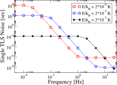
Figure 2: (Color online) Log-log plot of the low frequency polarization noise of a single two level system given by Eq. (56) versus frequency for three different values of the TLS energy splitting as shown in the legend. For all 3 cases, $T=0.1$ K, $I/I_{c}=10^{-4}$, $\Omega=E/\hbar$, and $\Delta=\Delta_{0}=E/\sqrt{2}$.

In Fig. 2, we show the spectral density $S_{P_{||}}(\omega)/\langle\delta P_{0}^{2}\rangle$ of polarization fluctuations of a single TLS at low frequencies. We consider three values of the TLS energy splitting as shown in the legend. In the low frequency range, the noise spectrum is dominated by the relaxation contribution which is a Lorentzian. Thus the noise spectrum is flat for $\omega\ll 1/T_{1}$. As the frequency increases, it rolls over at $\omega\sim 1/(T_{1})$, and goes as $1/\omega^{2}$ for $\omega>1/T_{1}$. At very high frequencies $\left(\omega>|E/\hbar|\right)$, it saturates to a constant (white noise) due to the resonance terms. In addition, we find that the low frequency noise is independent of electric field intensity ratio $I/I_{c}$ and the angular frequency $\Omega$ of the ac driving field.

The contribution of the resonance terms to the noise spectrum is negligible at low frequencies ($\omega\ll E/\hbar$) as expected from simple numerical estimates. However these resonance terms become important at high frequencies as shown in Fig. 3. The peaks appear when the resonance condition $\omega=\omega_{0}=E/\hbar$ is satisfied. The plot in Fig. 3 was obtained for the low value of the ratio $I/I_{c}=10^{-4}$. No noticeable differences were obtained when the ratio was increased to values as high as $10^{7}$ (not shown).

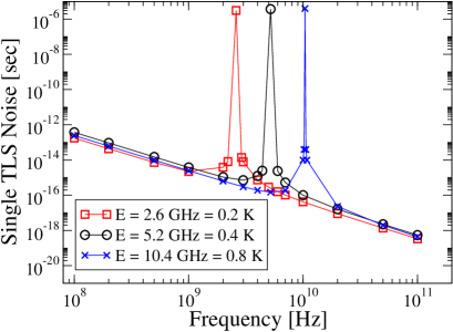
Figure 3: (Color online) Log-log plot of the high frequency polarization noise of a single two level system given by Eq. (56) versus frequency for three different TLS energy splittings. The peaks appears when the resonance condition $\omega=E/\hbar$ is satisfied. In all three cases, $T=0.1$ K, $I/I_{c}=10^{-4}$, $\Omega=E/\hbar$ and $\Delta=\Delta_{0}=E/\sqrt{2}$. No noticeable difference was obtained for $I/I_{c}=10^{7}\gg 1$ (not shown).

Figure 4 shows the polarization noise power of a single two level system over a broad range of frequencies that covers both the resonance and relaxation contributions. At low frequencies there is a plateau. Between 100 kHz and 1 GHz, the noise spectrum decreases as $1/\omega^{2}$ due to the Lorentzian associated with the relaxation contribution. At higher frequencies there is a resonance peak at $\omega=E/\hbar$.

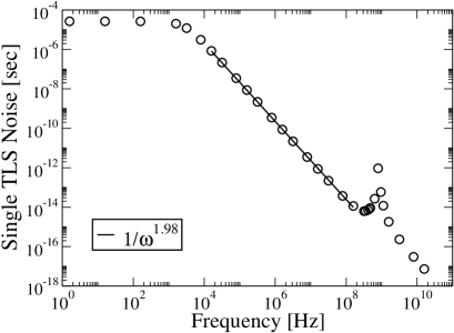
Figure 4: Log-log plot of the polarization noise of a single two level system given by Eq. (56) versus frequency for a broad range of frequencies. $E$ = 5.2 GHz = 0.4 K, $I/I_{c}=10^{-4}$, $\Omega=E/\hbar$, and $\Delta=\Delta_{0}=E/\sqrt{2}$.

The effect of TLS saturation can be seen at high frequencies in the plot of the noise of a single TLS versus the ratio $I/I_{c}$ as shown in Fig. 5. We plotted the spectral density of polarization fluctuations of an individual TLS given by Eq. (56) at a fixed high frequency ($\omega/2\pi=9$ GHz) versus $I/I_{c}$.

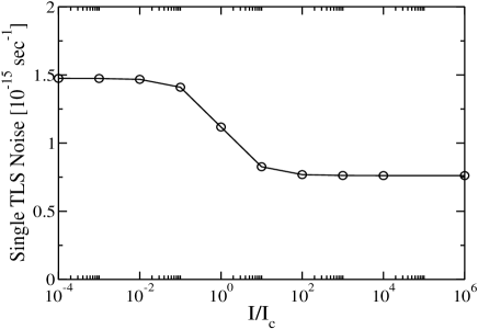
Figure 5: Log-linear plot of the high frequency polarization noise for a single two level system given by Eq. (56) versus $I/I_{c}$. The amplitude of the noise decreases by a factor of two as saturation is achieved for $I/I_{c}>1$. $\omega/2\pi=9$ GHz, $E/h=\Omega/2\pi=10$ GHz, $\Delta=\Delta_{0}=E/\sqrt{2}$, and $T=0.1$ K.

Notice that the noise is constant as long as $I\ll I_{c}$, then decreases when the electric field intensity increases to a value comparable to the critical intensity, and reaches a value which is half the previous one for $I\gg I_{c}$. This is in agreement with our estimates from Section V where we saw that as $I/I_{c}$ increases, $\rho_{--}$ decreases by a factor of 2 from a value close to 1 to a value close to 0.5 when the TLS are saturated.

VI.2 Polarization and Charge Noise of an Ensemble of TLS Fluctuators

Until now we have analyzed the contribution of a single fluctuator to the polarization noise spectrum. We now average the polarization noise of a single fluctuator over an ensemble of independent fluctuators in a volume $V_{o}$. The distribution function over TLS parameters was given in Eq. (8) as $P(\Delta,\Delta_{0})=P_{TLS}/\Delta_{0}$. Using this, we obtain:

$$\frac{S_{P_{||}}(\omega)}{\langle\delta P_{0}^{2}\rangle} =V_{o}\int_{\Delta_{min}}^{\Delta_{max}}\mbox{d}\Delta\int_{\Delta_{0,min}}^{\Delta_{0,max}}\mbox{d}\Delta_{0}P(\Delta,\Delta_{0})$$

$$\times\biggr{(}\frac{\Delta}{E}\biggr{)}^{2}\bigr{[}\frac{1}{\cosh^{2}(E/2k_{B}T)}]\frac{T_{1}}{1+\omega^{2}T_{1}^{2}}$$

$$+\biggr{(}\frac{\Delta_{0}}{E}\biggr{)}^{2}\biggr{[}(\rho_{--})\frac{T_{2}}{1+(\omega-E/\hbar)^{2}T_{2}^{2}}$$

$$+(\rho_{++})\frac{T_{2}}{1+(\omega+E/\hbar)^{2}T_{2}^{2}}\biggr{]}+{\rm dc\;term}$$

$$\equiv V_{o}J(\omega;\Omega,T,I/I_{c})+{\rm dc\;term},$$ (57)

where $J(\omega;\Omega,T,I/I_{c})$ is the result of integrating over the distribution of TLS parameters $\Delta$ and $\Delta_{0}$.

To obtain the charge noise $S_{Q}(\omega)$ from the polarization noise, we use Eq. (27) with

$$\langle\delta P_{0}^{2}\rangle = \left\langle\left(\frac{2p\cos\theta_{0}}{V_{o}}\right)^{2}\right\rangle$$ (58)

$$= \frac{4p^{2}}{3V_{o}^{2}}.$$ (59)

We obtain

$$\frac{S_{Q}(\omega)}{e^{2}}=\frac{4}{3}\bigr{(}\frac{p}{eL}\bigr{)}^{2}V_{o}J(\omega;\Omega,T,I/I_{c})+{\rm dc\;term}.$$ (60)

We can evaluate Eq. (60) numerically using $p=3.7$ D, $P_{TLS}=10^{45}$ (Jm³)^-1, $L=400$ nm, $A=40\times 800$ nm², $V_{o}=AL$, $\Delta_{min}=0$, $\Delta_{max}/k_{B}=\Delta_{0,max}/k_{B}=4$ K, and $\Delta_{0,min}/k_{B}=2\times 10^{-6}$ K. The results follow. We will drop the dc term from now on since it only affects the zero frequency noise.

VI.2.1 Low Frequency Charge Noise

Evaluating Eq. (60) produces the normalized low frequency ($\omega\ll|E/\hbar|$) charge noise spectrum $S_{Q}/e^{2}$ shown in Fig. 6. It is flat at very low frequencies $\omega T_{1}\ll 1$. As the frequency increases, it rolls over at $\omega\approx(T_{1,max})^{-1}$ and decreases as $1/f$ noise between approximately $10^{-3}$ and $10^{4}$ Hz. Here $T_{1,max}$ is the maximum value of $T_{1}$. For $T=0.1$ K, $T_{1,max}\sim 10^{4}$ s.

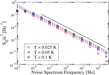
Figure 6: (Color online) Log-log plot of the low frequency charge noise $S_{Q}/e^{2}$ averaged over the TLS ensemble versus frequency for different temperatures. The symbols are the results of numerically evaluating Eq. (57) with $I/I_{c}=10^{-4}$ and $\Omega=10$ GHz. The dashed lines are the low frequency approximation given by Eq. (64). The solid line has a slope of $-1$ corresponding to a perfect $1/f$ spectrum. Between $10^{-3}$ and $10^{4}$ Hz, the noise spectrum is very close to $1/f$. For example, in this frequency range for $T=0.1$ K the noise spectrum goes as $1/(f^{1.02})$.

We can obtain an approximate analytic expression for the low frequency noise from Eq. (60) in the following way. By low frequency, we mean that $\omega\tau_{min}\ll 1$ and $\hbar\omega\ll E$. So we only keep the first term in $J(\omega;\Omega,T,I/I_{c})$ as defined by Eq. (57):

$$\frac{S_{Q}(\omega)}{e^{2}} \simeq \frac{4}{3}\bigr{(}\frac{p}{eL}\bigr{)}^{2}V_{o}\int_{\Delta_{min}}^{\Delta_{max}}\mbox{d}\Delta\int_{\Delta_{0,min}}^{\Delta_{0,max}}\mbox{d}\Delta_{0}P(\Delta,\Delta_{0})$$ (61)

$$\times \biggr{(}\frac{\Delta}{E}\biggr{)}^{2}\bigr{[}\frac{1}{\cosh^{2}(E/2k_{B}T)}]\frac{T_{1}}{1+\omega^{2}T_{1}^{2}}$$

We change variables to the TLS energy splitting $E$ and the relaxation time $T_{1}$. Using

$$\frac{\Delta^{2}}{E^{2}}=1-\left(\frac{\tau_{min}}{T_{1}}\right),$$ (62)

we obtain

$$\frac{S_{Q}(\omega)}{e^{2}} \simeq \frac{4}{3}\bigr{(}\frac{p}{eL}\bigr{)}^{2}V_{o}\int_{\tau_{min}}^{\infty}dT_{1}\int_{0}^{E_{max}}dE\;P(E,T_{1})$$ (63)

$$\times \left[1-\frac{\tau_{min}}{T_{1}}\right]\frac{1}{\cosh^{2}\left(E/2k_{B}T\right)}\frac{T_{1}}{1+\omega^{2}T_{1}^{2}}$$

where $P(E,T_{1})$ is given by Eq. (6). Using $\left(\tau_{min}/T_{1}\right)\ll 1$ yields

$$\frac{S_{Q}(\omega)}{e^{2}} \simeq \frac{4}{3}\bigr{(}\frac{p}{eL}\bigr{)}^{2}\frac{V_{o}P_{TLS}}{2}\int_{0}^{E_{max}}dE\frac{1}{\cosh^{2}\left(E/2k_{B}T\right)}$$ (64)

$$\times \int_{\tau_{min}}^{\infty}\frac{dT_{1}}{1+\omega^{2}T_{1}^{2}}$$

$$\simeq \frac{2\pi}{3}V_{o}P_{TLS}\left(\frac{p}{eL}\right)^{2}\frac{k_{B}T}{\omega}$$

Thus we obtain $1/f$ noise that goes linearly with temperature. As Fig. 6 shows, this expression for the low frequency noise gives good agreement with our numerical evaluation of Eq. (57). Eq. (64) also agrees with KoganKogan (1996), and Faoro and IoffeFaoro and Ioffe (2006). To estimate the value of $S_{Q}/e^{2}$ from Eq. (64), we use $p=3.7$ D, $P_{TLS}\approx 10^{45}$ (Jm³)^-1, $L=400$ nm, $A=40\times 800$ nm², and $V_{o}=AL$. At $T=0.1$ K and $f=1$ Hz, we obtain $S_{Q}/e^{2}=2\times 10^{-7}$ Hz^-1, which is comparable to the experimental value of $4\times 10^{-6}$ Hz^-1 deduced from current noise. Astafiev et al. (2006) The magnitude of this noise estimate is also in good agreement with our numerical result from Eq. (60), i.e., $S_{Q}(f=1$ Hz$)/e^{2}=2\times 10^{-7}$ Hz^-1.

We can also obtain this $1/f$ noise result with the following simple calculation. Consider an electric dipole moment ${\bf p}$ in a parallel plate capacitor at an angle $\theta_{0}$ with respect to the $z-$axis which is perpendicular to the electrodes that are a distance $L$ apart. Assume that the electrodes are at the same voltage. When the dipole flips by 180^o, the induced charges on the superconducting electrodes change from $\mp p\cos\theta_{0}/L$ to $\pm p\cos\theta_{0}/L$. Let $\delta Q$ denote the magnitude of the charge fluctuations. Then $\delta Q=|2p\cos\theta_{0}/L|$. Hence the charge of the Josephson junction capacitor produces a simple two state random telegraph signal which switches with a transition rate $\tau^{-1}$ given by the sum of the rates of transitions up and down.Kogan (1996) The charge noise spectral density is Kogan (1996)

$$S_{Q}^{(i)}(\omega) =2\int_{-\infty}^{\infty}{\mbox{d}(t_{1}-t_{2})\mbox{e}^{i\omega(t_{1}-t_{2})}\langle\delta Q(t_{1})\delta Q(t_{2})\rangle}$$

$$=\langle(\delta Q)\rangle^{2}\frac{4w_{1}w_{2}\tau}{1+\omega^{2}\tau^{2}}~{}~{},$$ (65)

where the superscript $i$ refers to the $i$th TLS in the substrate or tunnel barrier, and $w_{1}$ ($w_{2}$) is the probability of being in the lower (upper) state of the TLS. In order to average over TLS, we recall from Eq. (6) that the distribution function of TLS parameters can be written in terms of the energy and relaxation times:Phillips (1981)

$$P(E,\tau)=\frac{P_{TLS}}{(2\tau\sqrt{1-\tau_{min}/\tau})}.$$ (66)

At low frequencies $\omega\tau_{min}\ll 1$, the main contribution to the spectral density comes from slowly relaxing TLS for which $P(E,\tau)\simeq P_{TLS}/(2\tau)$. Therefore, the charge noise of an ensemble of independent fluctuators is

$$S_{Q}(\omega) \simeq V_{o}\int_{\tau_{min}}^{\infty}\mbox{d}\tau\int_{0}^{E_{max}}\mbox{d}E~{}\frac{P_{TLS}}{2\tau}$$

$$\times\frac{\langle\delta Q^{2}\rangle}{\cosh^{2}(E/2k_{B}T)}\frac{\tau}{1+\omega^{2}\tau^{2}}~{}~{}.$$ (67)

$\langle\delta Q^{2}\rangle$ is the square of the amplitude of charge fluctuations averaged over TLS dipole orientations. We assume that $\langle\delta Q^{2}\rangle$ is independent of $E$ and $\tau$. At low temperatures ($k_{B}T\ll E_{max}$) and low frequencies ($\omega\tau_{min}\ll 1$), we recover Eq. (64) which describes $1/f$ charge noise that goes linearly with temperature.

Still another way to obtain low frequency $1/f$ noise is the following. At low frequencies the system is in thermal equilibrium, and we can use Eq. (14) from Section III:

$$\frac{S_{Q}(\omega)}{e^{2}}=\frac{2k_{B}T}{e^{2}/2C}\frac{\tan\delta}{\omega}.$$ (68)

The TLS contribution to the dielectric loss tangent $\tan\delta$ was calculated by previous workers Phillips (1981); Classen et al. (1994); Hunklinger and Arnold (1976) who considered fluctuating TLS with electric dipole moments. They found

$$\tan\delta=\frac{\pi p^{2}P_{TLS}}{6\varepsilon^{\prime}}$$ (69)

where $\varepsilon^{\prime}$ is the real part of the dielectric permittivity and $P_{TLS}$ the constant TLS density of states. By plugging Eq. (69) into Eq. (68) and using Eq. (13) and $V_{o}=AL$, we recover Eq. (64).

VI.2.2 High Frequency Charge Noise

Evaluating Eq. (60) numerically at high frequencies yields the normalized charge noise spectrum shown in Fig. 7. We have plotted the contributions coming from the relaxation term and the two resonance terms separately. As we described in the previous subsection, the relaxation term dominates at low frequencies and gives $1/f$ noise. In the high frequency range shown in Fig. 7, the relaxation term produces $1/f^{2}$ noise. On the other hand, the resonance terms produce white (flat) noise that dominates at high frequencies. The two curves cross at approximately 10 MHz.

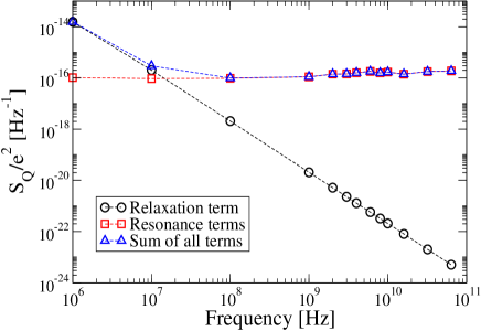
Figure 7: (Color online) Log-log plot of the high frequency charge noise $S_{Q}/e^{2}$ averaged over the TLS ensemble versus frequency. The contributions of the relaxation term and the resonance terms are plotted separately. The noise spectrum becomes white noise at frequencies $\stackrel{{\scriptstyle>}}{{\sim}}10$ MHz. The results were obtained using $T=0.1$ K, $\Omega=10$ GHz, and $I/I_{c}=10^{7}$.

Regarding the temperature dependence, we note that while the low frequency $1/f$ noise is proportional to temperature, the high frequency white noise decreases gradually with increasing temperature as shown in Fig. 8. To understand this temperature dependence, note that at high frequencies the resonant terms dominate. These are the terms in Eq. (57) with $(\omega\pm E/\hbar)$ in the denominator. The dominant contribution to the integral occurs at resonance ($\omega=E/\hbar$) where the temperature dependence of the integrand goes as $T_{2}\sim 1/T$ and decreases as the temperature increases. However, this decrease is much stronger than seen in the ensemble averaged noise shown in Fig. 8. This may be because in obtaining the ensemble averaged noise, one adds terms away from resonance which have the opposite trend and increase with increasing temperature as $T_{2}^{-1}\sim T$.

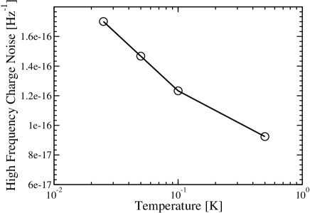
Figure 8: Plot of the high frequency charge noise $S_{Q}(\omega)/e^{2}$ averaged over the TLS ensemble versus temperature. Notice that the noise decreases gradually with increasing temperature. This plot was obtained for $\omega=10$ GHz, a driving frequency of $\Omega=10$ GHz, and $I/I_{c}=10^{7}$.

In Fig. 9 we show our cumulative numerical results for the charge noise spectrum at both low and high frequencies. As we mentioned previously, there is no noticeable dependence on the electric field intensity ratio $I/I_{c}$ at either low or high frequencies.

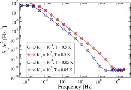
Figure 9: (Color online) Log-log plot of the charge noise $S_{Q}(\omega)/e^{2}$ averaged over the TLS ensemble versus frequency. Notice that the results for large and small values of $I/I_{c}$ overlap. We have considered two temperatures, 0.5 K and 0.05, respectively, and the driving frequency was $\Omega=10$ GHz.

Our result of white noise at high frequencies disagrees with the experiments by Astafiev et al. Astafiev et al. (2004) who concluded that the noise increases linearly with frequency. However, we caution that the experiments were done under different conditions from the calculation. The experimentalists Astafiev et al. (2004) applied dc pulses with Fourier components up to a few GHz, possibly saturating TLS with energy splittings in this frequency range. They relied on a Landau-Zener transition to excite the qubit which had a much larger energy splitting, ranging up to 100 GHz, and measured the decay rate $\Gamma_{1}$ of the qubit. Then they used $\Gamma_{1}$ to deduce the charge noise spectrum at frequencies equal to the qubit splitting by using a formula Schoelkopf et al. (2002) derived assuming a stationary state. It is not clear whether it is valid to assume a stationary state in the presence of dc pulses which lasted for a time ($\sim$ 100 ps) comparable to the lifetime of the qubit.

In contrast, in calculating noise spectra, we make the customary assumption of stationarity. We relate the charge noise spectra to the response to an ac drive for a broad range of frequencies. AC driving of qubits have been used in both theoretical Shnirman et al. (1997); You and Nori (2003); Ashhab et al. (2007) and experimental studies Nakamura et al. (2001); Oliver et al. (2005); Sillanpäa et al. (2006); Berns et al. (2006) of qubits. It would be interesting to measure the frequency and temperature dependence of the charge noise in Josephson qubits in the presence of ac driving since no such measurements have been done.

VII Summary

To summarize, we have studied the effect of the saturation of TLS by electromagnetic waves on qubit charge noise. Using the standard theory of two level systems with a flat density of states, we find that the charge noise at low frequencies is $1/f$ noise and is insensitive to the saturation of the two level systems. In addition the low frequency charge noise increases linearly with temperature. As one approaches high frequencies, the charge noise plateaus to white noise with a very weak dependence on the driving frequency $\Omega$ and the ratio $I/I_{c}$. We found that the high frequency charge noise decreases slightly with increasing temperature.

Finally we note that while we have been considering a Josephson junction qubit, our results on charge and polarization noise have not relied on the superconducting properties of the qubit. So our results are much more general and pertain to the charge noise produced by fluctuating TLS in a capacitor or substrate subject to a driving ac electric field in steady state.

This work was supported by the Disruptive Technology Office under grant W911NF-04-1-0204, and by DOE grant DE-FG02-04ER46107.

$\dagger$Current address: Radiation Physics Division, Department of Radiation Oncology, Stanford University, Stanford, CA 94305-5847

VIII Appendix: Derivation of the Charge Induced on the Electrodes by a Dipole

In this appendix we derive Eq. (1) which gives the magnitude of the charge induced on the electrodes by a dipole Eq. (1). Rather than use image charges which leads to an infinite sum, we follow Purcell.Purcell (1965) We start by considering the simple problem of a charge $q$ between two conducting plates connected by a wire so that they are at the same electric potential. The plates are parallel to the $xy$ plane and separated by a distance $L$. The sum of the induced charges is $-q$. Let $d_{u}$ ($d_{\ell}$) be the perpendicular distance from the charge $q$ to the upper (lower) plate. Let $-q_{u}$ ($-q_{\ell}$) be the charge induced on the upper (lower) plate so that $-q_{u}-q_{\ell}=-q$. Notice that if the charge between the plates is doubled to $2q$ such that $d_{u}$ and $d_{\ell}$ stay the same as before, the ratio $q_{u}/q_{\ell}$ stays the same even though the total induced charge is $-2q$. So let us replace $q$ by a conducting plate with charge density $\sigma$ while still maintaining the distances $d_{u}$ and $d_{\ell}$. The total induced charge density is $-2\sigma=-\sigma_{u}-\sigma_{\ell}$ where $-\sigma_{u}$ and $-\sigma_{\ell}$ are the induced charge densities on the upper and lower plates, respectively. Notice that

$$\frac{\sigma_{u}}{\sigma_{\ell}}=\frac{q_{u}}{q_{\ell}}$$ (70)

Using Gauss’ Law to find the electric field and the fact that the voltage difference between the middle plate and the upper plate equals the voltage difference between the middle plate and the lower plate yields

$$\frac{\sigma_{u}}{\sigma_{\ell}}=\frac{d_{\ell}}{d_{u}}$$ (71)

Now we return to the problem of the charge induced on the plates due a point charge $q$ between the plates. From Eqs. (71) and (70), we obtain

$$q_{u}=q\frac{d_{\ell}}{L}$$ (72)

and

$$q_{\ell}=q\frac{d_{u}}{L}$$ (73)

Now suppose we have a dipole between the two conducting plates at the same potential. The dipole consists of two equal and opposite charges $q_{+}=q$ and $q_{-}=-q$ separated by a distance $d$. The magnitude of the dipole moment is $p=qd$, and $\theta$ is the angle between the z-axis and the dipole moment ${\bf p}$. Let $d_{u+}$ ($d_{\ell+}$) be the distance between $q_{+}=q$ and the upper (lower) plate, and let $d_{u-}$ ($d_{\ell-}$) be the distance between $q_{-}=-q$ and the upper (lower) plate. Then the charge induced on the lower plate is $-q_{\ell}$ where

$$q_{\ell} = \frac{q}{d}\left(d_{u+}-d_{u-}\right)$$ (74)

$$= -\frac{p\cos\theta}{L}$$

Similarly the charge induced on the upper plate is $-q_{u}$ where

$$q_{u}=\frac{p\cos\theta}{L}$$ (75)

Thus we recover Eq. (1) for $Q$, the magnitude of the charge induced on each electrode.

References

- Vion et al. (2002) D. Vion, A. Aassime, A. Cottet, P. Joyez, H. Pothier, C. Urbina, D. Esteve, and M. H. Devoret, Science 296, 886 (2002).
- Yu et al. (2002) Y. Yu, S. Han, X. Chu, S. Chu, and Z. Wang, Science 296, 889 (2002).
- Martinis et al. (2002) J. M. Martinis, S. Nam, J. Aumentado, and C. Urbina, Phys. Rev. Lett. 89, 117901 (2002).
- Chiorescu et al. (2003) I. Chiorescu, Y. Nakamura, C. J. P. M. Harmans, and J. E. Mooij, Science 299, 1869 (2003).
- Pashkin et al. (2003) Y. A. Pashkin, Y. Yamamoto, O. Astafiev, Y. Nakamura, D. V. Averin, and J. S. Tsai, Nature 421, 823 (2003).
- Berkley et al. (2003) A. J. Berkley, H. Xu, R. C. Ramos, M. A. Gubrud, F. W. Strauch, P. R. Johnson, J. R. Anderson, A. J. Dragt, C. J. Lobb, and F. C. Wellstood, Science 300, 1548 (2003).
- Simmonds et al. (2004) R. W. Simmonds, K. M. Lang, D. A. Hite, S. Nam, D. P. Pappas, and J. M. Martinis, Phys. Rev. Lett. 93, 077003 (2004).
- Martinis et al. (2005) J. M. Martinis, K. B. Cooper, R. McDermott, M. Steffen, M. Ansmann, K. D. Osborn, K. Cicak, S. Oh, D. P. Pappas, R. W. Simmonds, et al., Phys. Rev. Lett. 95, 210503 (2005).
- Zimmerli et al. (1992) G. Zimmerli, T. M. Eiles, R. L. Kautz, and J. M. Martinis, Appl. Phys. Lett. 61, 237 (1992).
- Visscher et al. (1995) E. H. Visscher, S. M. Verbrugh, J. Lindeman, P. Hadley, and J. E. Mooij, Appl. Phys. Lett. 66, 305 (1995).
- Zorin et al. (1996) A. B. Zorin, F. J. Ahlers, J. Niemeyer, T. Weimann, H. Wolf, V. A. Krupenin, and S. V. Lotkhov, Phys. Rev. B 53, 13682 (1996).
- Kenyon et al. (2000) M. Kenyon, C. J. Lobb, and F. C. Wellstood, J. Appl. Phys. 88, 6536 (2000).
- Astafiev et al. (2006) O. Astafiev, Y. A. Pashkin, Y. Nakamura, T. Yamamoto, and J. S. Tsai, Phys. Rev. Lett. 96, 137001 (2006).
- Shnirman et al. (2005) A. Shnirman, G. Schon, I. Martin, and Y. Makhlin, Phys. Rev. Lett. 94, 127002 (2005).
- Faoro et al. (2005) L. Faoro, J. Bergli, B. L. Altshuler, and Y. M. Galperin, Phys. Rev. Lett. 95, 046805 (2005).
- Faoro and Ioffe (2006) L. Faoro and L. B. Ioffe, Phys. Rev. Lett. 96, 047001 (2006).
- Hunklinger and Arnold (1976) S. Hunklinger and W. Arnold, in Physical Acoustics: Principles and Methods, vol.12, edited by W. P. Mason and R. N. Thurston (Academic Press, New York, 1976), pp. 155–215.
- Golding et al. (1976) B. Golding, J. E. Graebner, and R. J. Schutz, Phys. Rev. B 14, 1660 (1976).
- Graebner et al. (1983) J. E. Graebner, L. C. Allen, B. Golding, and A. B. Kane, Phys. Rev. B 27, 3697 (1983).
- Schickfus and Hunklinger (1977) M. V. Schickfus and S. Hunklinger, Phys. Lett. A 64, 144 (1977).
- Astafiev et al. (2004) O. Astafiev, Y. A. Pashkin, Y. Nakamura, T. Yamamoto, and J. S. Tsai, Phys. Rev. Lett. 93, 267007 (2004).
- Phillips (1981) W. A. Phillips, Amorphous Solids (Springer–Verlag, New York, 1981).
- Classen et al. (1994) J. Classen, C. Enss, C. Bechinger, and S. Hunklinger, Ann. Phys. 3, 315 (1994).
- Golding et al. (1979) B. Golding, M. v. Schickfus, S. Hunklinger, and K. Dransfeld, Phys. Rev. Lett. 43, 1817 (1979).
- Phillips (1987) W. A. Phillips, Rep. Prog. Phys. 50, 1657 (1987).
- Forster (1990) D. Forster, Hydrodynamic Fluctuations, Broken Symmetry and Correlation Functions (Perseus Books, need address, 1990).
- Jäckle et al. (1976) J. Jäckle, L. Piche, W. Arnold, and S. Hunklinger, J. Non-Cryst. Solids 20, 365 (1976).
- Slichter (1990) C. P. Slichter, Principles of Magnetic Resonance (Springer–Verlag, Berlin, 1990), 3rd ed.
- Redfield (1957) A. G. Redfield, IBM J. Res. Dev. 1, 19 (1957).
- Bernard et al. (1979) L. Bernard, L. Piche, G. Schumacher, and J. Joffrin, J. Low Temp. Phys. 35, 411 (1979).
- Carruzzo et al. (1994) H. M. Carruzzo, E. R. Grannan, and C. C. Yu, Phys. Rev. B 50, 6685 (1994).
- Machlup (1954) S. Machlup, J. Appl. Phys. 25, 341 (1954).
- Kogan (1996) S. Kogan, Electronic Noise and Fluctuations in Solids (Cambridge University Press, Cambridge, 1996).
- Schoelkopf et al. (2002) R. J. Schoelkopf, A. A. Clerk, S. M. Girvin, K. W. Lehert, and M. Devoret, in Quantum Noise in Mesoscopic Physics, edited by Y. V. Nazarov (Kluwer, Dordrecht, 2002), pp. 175–203.
- Shnirman et al. (1997) A. Shnirman, G. Schön, and Z. Hermon, Phys. Rev. Lett. 79, 2371 (1997).
- You and Nori (2003) J. Q. You and F. Nori, Phys. Rev. B 68, 064509 (2003).
- Ashhab et al. (2007) S. Ashhab, J. R. Johansson, A. M. Zagoskin, and F. Nori, Phys. Rev. A 75, 063414 (2007).
- Nakamura et al. (2001) Y. Nakamura, Y. A. Pashkin, and J. S. Tsai, Phys. Rev. Lett. 87, 246601 (2001).
- Oliver et al. (2005) W. D. Oliver, Y. Yu, J. C. Lee, K. K. Berggren, L. S. Levitov, and T. P. Orlando, Science 310, 1653 (2005).
- Sillanpäa et al. (2006) M. Sillanpäa, T. Lehtinen, A. Paila, Y. Makhlin, and P. Hakonen, Phys. Rev. Lett. 96, 187002 (2006).
- Berns et al. (2006) D. M. Berns, W. D. Oliver, S. O. Valenzuela, A. V. Shytov, K. K. Berggren, L. S. Levitov, and T. P. Orlando, Phys. Rev. Lett. 97, 150502 (2006).
- Purcell (1965) E. M. Purcell, Electricity and Magnetism (McGraw-Hill, New York, 1965).