Langevin approach to synchronization of hyperchaotic time-delay dynamics

Abstract

In this paper, we characterize the synchronization phenomenon of hyperchaotic scalar non-linear delay dynamics in a fully-developed chaos regime. Our results rely on the observation that, in that regime, the stationary statistical properties of a class of hyperchaotic attractors can be reproduced with a linear Langevin equation, defined by replacing the non-linear delay force by a delta-correlated noise. Therefore, the synchronization phenomenon can be analytically characterized by a set of coupled Langevin equations. We apply this formalism to study anticipated synchronization dynamics subject to external noise fluctuations as well as for characterizing the effects of parameter mismatch in a hyperchaotic communication scheme. The same procedure is applied to second order differential delay equations associated to synchronization in electro-optical devices. In all cases, the departure with respect to perfect synchronization is measured through a similarity function. Numerical simulations in discrete maps associated to the hyperchaotic dynamics support the formalism.

I Introduction

In the last decades, synchronization of chaotic dynamics became a subject that has attracted of lot of attention book ; fujisaka ; pikovsky1 ; pikovsky2 ; grassberger ; pecora ; carroll . In fact, from a theoretical point of view, this phenomenon seems to contradict the inheriting sensibility to initial conditions of chaotic dynamics. On the other hand, the interest in this kind of phenomenon comes from the possibility of using the unpredictable chaotic trajectories as a carrier signal in communication channels. In this context, high dimensional systems with multiple positive Lyapunov exponents, i.e., hyperchaotic dynamics rossler , have been proposed as a resource for improving the security in the communication schemes. Synchronization of hyperchaotic systems has therefore also become an area of active research kocarev ; peng ; laiR ; ali ; parker .

Chaotic dynamics described by differential delay equations arise in the description of many different kind of situations, such as physiology mackey ; foss , biology donald , economy economy , laser physics ikeda1 ; ikeda2 ; laser ; hanna ; gibbs , etc. As is well known, a high dimensional chaotic attractor characterizes these infinite dimensional systems. It has been shown that the Lyapunov dimension of the attractor is proportional to the characteristic delay time of the dynamics gibbs ; farmer ; procaccia ; berreR . Therefore, “synchronization of hyperchaotic nonlinear delay dynamics” has also been extensively explored from both a theoretical point of view as well as a resource for communication schemes porte ; lai ; yinghai ; rhodes . A new aspect introduced in this case is the possibility of synchronizing two chaotic dynamics with a time shift, giving rise to the phenomenon of anticipated voss1 ; voss2 ; voss3 ; pyragas ; masoller ; zanette ; mirasso ; tang ; toral ; shore ; heil (or retarded) synchronization, i.e., one of the chaotic systems (slave or receiver system) follows the chaotic trajectory of the other one (master or transmitter system) with an advanced (or retarded) time shift.

In any real experimental setup where chaotic synchronization is observed one is naturally confronted with two undesirable effects that avoid reaching a perfectly synchronized regime. The characteristic parameters of both systems are not exactly the same, small parameter mismatch may induce clearly observable effects colet ; mismatch ; mar . Also, departure with respect to the perfectly synchronized manifold may also be due to intrinsic noise fluctuations present in both systems tufillaro ; chua . Both effects have been analyzed in the literature. Nevertheless, due to the chaotic character of the dynamics, in general it is hard to obtain an analytical estimation of these effects, which in fact may depend on the specific nature of the chaotic systems as well as on the coupling scheme used to achieve synchronization.

The aim of this paper is to provide a simple analytical description of the phenomenon of synchronization of hyperchaotic delay dynamics, considering realistic situations such as the presence of parameter mismatch as well as the presence of intrinsic noise fluctuations in both synchronized systems. We demonstrate that this goal can be achieved when the synchronized dynamics are in a fully-developed chaos regime gyorgyi . In this situation, the corresponding chaotic attractor does not have any stable periodic orbit and its basin of attraction fills out almost the whole available domain. These properties suggest that the nonlinear delay contribution terms of the chaotic dynamics may be statistically equivalent to an ergodic noise source. As demonstrated in Ref. berre ; berre1 , this property, in a long time limit and depending on the characteristic parameter values, is in fact valid for a broad class of scalar delay dynamics. Therefore, our main idea consists in replacing the full set of coupled delay chaotic evolutions that lead to synchronization by a set of correlated Langevin evolutions obtained from the original chaotic ones after replacing the nonlinear delay contributions by a noise term. Since the final Langevin equations are linear, their statistical properties can be obtained in an exact analytical way, providing a simple framework for characterizing the synchronization phenomenon. Departure with respect to perfect synchronization is characterized in terms of a similarity function kurths , which measures the degree of correlation between the quasi-synchronized dynamics.

The paper is organized as follows. In Sec. II we review the conditions under which hyperchaotic delay dynamics can be represented by a Langevin dynamics. In Sec. III we analyze the phenomenon of anticipated synchronization when perturbed by external additive noises. In Sec. IV we analyze the effect of parameters mismatch in a hyperchaotic communication scheme porte . In Sec. V we study a set of second order differential delay equations associated to an electro-optical laser device colet under the effect of parameter mismatch and under the action of external additive noises. In all cases, we present numerical simulations that sustain our theoretical results. In Sec. VI we give the conclusions.

II Langevin approach to hyperchaotic delay dynamics in the fully-developed chaos regime

We will consider scalar nonlinear delay evolutions with the structure

$$\dot{u}(t)=-\gamma u(t)+\beta f[u(t-T)]+\mathrm{I}(t).$$ (1)

Here, $\gamma$ defines a dissipative time scale and $T$ is the characteristic time delay. The parameter $\beta$ controls the weights of the nonlinear function $f(x),$ which is assumed to be oscillatory or at least exhibiting many different extrema notaReferee . The term $\mathrm{I}(t)$ represents an extra inhomogeneous contribution that may corresponds to a stationary Gaussian white noise (Sec. III), a deterministic signal (Sec. IV) or even it may be a linear functional of the process $u(t)$ (Sec. V).

The parameter $\beta T$ may be considered as a complexity control parameter. In fact, when $\beta T\gg 1,$ the dynamic reaches a fully-developed chaos regime, where the stationary statistical properties of the corresponding attractor can be reproduced with a linear Langevin equation berre ; berre1 . This property can be understood by integrating Eq. (1), in the long time limit $(\gamma t\gg 1),$ as

$$\tilde{u}(t)\approx\int_{0}^{t}dt^{\prime}e^{-\gamma(t-t^{\prime})}f[\beta\tilde{u}(t^{\prime}-T)+\mathrm{\tilde{I}}(t^{\prime}-T)],$$ (2)

where $\tilde{u}(t)=[u(t)-\mathrm{\tilde{I}}(t)]/\beta,$ and $\mathrm{\tilde{I}}(t)$ is defined by $\mathrm{\tilde{I}}(t)\equiv\int_{0}^{t}dt^{\prime}e^{-\gamma(t-t^{\prime})}\mathrm{I}(t^{\prime}).$ Then, by writing the integral operation over $f(x)$ as a discrete sum, $\int_{0}^{t}dt^{\prime}g(t^{\prime})\rightarrow\sum_{j}dt^{\prime}g(jdt^{\prime}),$ one realizes that $\tilde{u}(t)$ may be considered as the result of the addition of many “statistically independent”contributions. This last property follows from the fact that $f[\beta x]$ oscillates so fast that it behaves as a driving random force. The characteristic correlation time [in units of time $1/\gamma$] of the nonlinear force $f[\beta x]$ is of order $\gamma/\beta$ berre ; berre1 . When the correlation time is the small time-scale of the problem, i.e., much shorter than the characteristic delay time, $\gamma/\beta\ll\gamma T,$ and consistently much shorter than the characteristic dissipative time, $\gamma/\beta\ll 1,$ the statistical independence of the different contributions follows. Notice that this last property is independent of the structure of the inhomogeneous term $\mathrm{\tilde{I}}(t),$ which only introduce a shift in the argument of $f[\beta x].$

From the previous analysis, in the parameters region $\beta T\gg 1$ and $\gamma/\beta\ll 1,$ the central limit theorem kampen tell us that $\tilde{u}(t)$ is a Gaussian process. Due to this characteristic, this regime is also named Gaussian chaos. Only when $\mathrm{\tilde{I}}(t-T)$ is a non-linear function (functional) of $u(t)$ berre1 , the long time statistic may depart from a Gaussian one.

The lack of correlation between the different contributions of the “chaotic force” $f[\beta\tilde{u}(t-T)+\mathrm{\tilde{I}}(t-T)],$ allows to introduce the following Ansatz. In the fully-developed chaos regime, “the long time statistical properties” of $u(t)$ can be equivalently obtained from Eq. (2) after replacing the chaotic force by a noise contribution $(\beta f[\tilde{u}(t-T)+\mathrm{\tilde{I}}(t-T)]\rightarrow\eta(t-T)),$ delivering the Langevin equation

$$\dot{u}(t)=-\gamma u(t)+\eta(t-T)+\mathrm{I}(t).$$ (3)

The noise $\eta(t)$ must have the same statistical properties as the delayed chaotic force. Since we are restricting our analysis to the Gaussian chaos regime, it is sufficient to map the first two statistical moments Markov

$$\overline{\eta(t)} = \lim_{t\rightarrow\infty}\beta\overline{f[u(t)]},$$ (4)

$$\overline{\eta(t+\tau)\eta(t)} = \lim_{t\rightarrow\infty}\beta^{2}\overline{f[u(t+\tau)]f[u(t)]}.$$ (5)

The limit operation ($\lim_{t\rightarrow\infty}$) is introduced because the statistical mapping is only valid in the long time regime. The overbar symbol denotes an average over realizations obtained from Eq. (1) with different initial conditions. Equivalently, since the chaotic attractor is ergodic (by definition of fully-developed chaos regime) when the inhomogeneous term is statistically stationary kampen , this average can also be considered as a time average. For example, $\lim_{t\rightarrow\infty}\overline{f[u(t)]}=\lim_{t\rightarrow\infty}(1/t)\int_{0}^{t}dt^{\prime}f[u(t^{\prime})].$

In agreement with the lack of correlation between the different contributions of the chaotic force, $\eta(t)$ can be approximated by a delta-correlated noise,

$$\overline{\eta(t)\eta(t^{\prime})}-\overline{\eta(t)}\ \overline{\eta(t^{\prime})}=\mathcal{A}\delta(t-t^{\prime}).$$ (6)

This white noise approximation applies for time intervals $(t-t^{\prime})$ larger than the characteristic time correlation $(\gamma/\beta)$ [in units of time $1/\gamma$] of the chaotic force berre ; berre1 , i.e., $\gamma(t-t^{\prime})>(\gamma/\beta).$

The coefficient $\mathcal{A}$ measures the amplitude of $f[u(t)].$ Clearly, $\mathcal{A}$ must be proportional to $\beta^{2}.$ Nevertheless, its exact value is not universal and depends on the specific function $f(x)$ berre as well as on the parameters that define the inhomogeneous term (see next Section).

When $\mathrm{I}(t)$ is defined by an external driving force, we will assume that

$$\overline{[\eta(t)-\overline{\eta(t)}]\mathrm{I}(t^{\prime})}=0,$$ (7)

i.e., the noise fluctuations representing the chaotic force and the inhomogeneous term are statistically uncorrelated. The plausibility of this assumption follows from the fact that the white nature of $\eta(t)$ only relies on the rapid oscillating nature of $f[\beta x]$ while it is not affected by the shift introduced by the functional $\mathrm{\tilde{I}}(t).$ Under this condition, the inhomogeneous contribution only affects the mean value of the Gaussian profile associated to $u(t).$

Finally, we will assume that $\overline{\eta(t)}=0.$ The validity of this condition only depends on the specific properties of the non-linear chaotic force. In fact, the rapid oscillating nature of $f[\beta x]$ allows to discarding the asymmetry introduced by $\mathrm{\tilde{I}}(t)$ [Eq.(2)]. As will become clear in the next section, the generalization to the case $\lim_{t\rightarrow\infty}\beta\overline{f[u(t)]}\neq 0$ can also be worked straightforwardly.

With the noise correlation Eq. (6), the stochastic evolution Eq. (3) becomes a (driven) Orstein-Ulenbeck process kampen . The statistical equivalence in the stationary and fully developed chaos regimes of the deterministic evolution Eq. (1) and the Langevin Eq. (3), (without the inhomogeneous term) was proved in Refs. berre ; berre1 . Clearly, this stochastic representation does not provide any new information about the chaotic dynamics. Nevertheless, in the next sections we will use this equivalence for formulating a simple framework that allows us to get an analytical characterization of the chaotic synchronization phenomenon for different realistic circumstances.

III Anticipated synchronization subject to external additive noises

In this section we will apply the previous Langevin representation of a hyperchaotic attractor to analyze the phenomenon of anticipated synchronization voss1 ; voss2 ; voss3 in the presence of external noise sources. We consider a complete replacement scheme toral , defined by the coupled chaotic evolutions

$$\dot{x}(t) = -\gamma x(t)+\beta f[x(t-T)]+\xi_{x}(t),$$ (8a)

$$\dot{y}(t) = -\gamma y(t)+\beta f[x(t)]+\xi_{y}(t).$$ (8b)

In this context, the variables $$x(t) y(t) \gamma \beta f(x).$$ and are referred as master and slave variables respectively. As before, is a constant dissipative rate, and measures the weight of the delay-nonlinear contribution

We have considered external noise sources, defined by the master and slave noises $\xi_{x}(t)$ and $\xi_{y}(t)$ respectively. We assume that their mean values are null $\left\langle\xi_{z}(t)\right\rangle=0,$ where $z=x,y,$ and $\left\langle\cdots\right\rangle$ denotes average over noise realizations. Furthermore, we assume that both noises are Gaussian, with correlations

$$\left\langle\xi_{z}(t)\xi_{z^{\prime}}(t^{\prime})\right\rangle=\mathcal{A}_{zz^{\prime}}\delta(t-t^{\prime}).$$ (9)

The “diffusion” coefficients satisfy the positivity constraint $\mathcal{A}_{xx}\mathcal{A}_{yy}-\mathcal{A}_{xy}\mathcal{A}_{yx}\geq 0,$ $(\mathcal{A}_{xy}=\mathcal{A}_{yx})$ kampen . These definitions allows to cover the case where both the master and slave variables are affected by intrinsic uncorrelated fluctuations, $\mathcal{A}_{xy}=0,$ as well as the case of correlated fluctuations $\mathcal{A}_{xy}>0.$ This last situation may be easily produced in any experimental setup. In particular, for $\mathcal{A}_{xx}=\mathcal{A}_{yy}=\mathcal{A}_{xy},$ the noises that drive the master and slave dynamics are exactly the same, i.e., Eq. (8) with $\xi_{x}(t)=\xi_{y}(t).$ This property follows by diagonalizing the matrix of diffusion noise coefficients $\{\{\mathcal{A}_{xx},\mathcal{A}_{xy}\},\{\mathcal{A}_{xy},\mathcal{A}_{yy}\}\}.$

As it is well known, in the absence of the external noises $\xi_{x}(t)$ and $\xi_{y}(t),$ the master-slave dynamics Eq. (8), after a time transient of order $1/\gamma,$ reach the synchronized manifold $x(t+T)=y(t).$ Therefore, the slave variable anticipates the behavior of the master variable. The achievement of this state is clearly affected by the presence of the external noises. The degree of departure with respect to the perfectly synchronized manifold can be measured with a similarity function, defined as kurths

$$S(\tau)\equiv\lim_{t\rightarrow\infty}\left[\frac{\langle\overline{[x(t+\tau)-y(t)]^{2}}\rangle}{[\langle\overline{x^{2}(t)}\rangle\langle\overline{y^{2}(t)}\rangle]^{1/2}}\right]^{1/2}.$$ (10)

As before, the overbar denotes an average with respect to the system initialization or equivalently a time average in the asymptotic regime. In the absence of the external noises, this object satisfies $S(T)=0,$ indicating that the perfectly synchronized state $x(t+T)=y(t)$ was achieved. In the presence of the noises, we expect $S(T)>0.$

The characterization of the behavior of the similarity function $S(\tau)$ from the evolution Eq. (8) is in principle a highly non trivial task. The major complication come from the chaotic nature of the master and slave dynamics. Even in the absence of the external noises, in general it is impossible to get an analytical expression for the similarity function. Nevertheless, if both dynamics are in the fully-developed chaos regime, from the previous section, we know that a simpler representation may be achieved. The Langevin approach to Eq. (8) reads

$$\dot{x}(t) = -\gamma x(t)+\eta(t-T)+\xi_{x}(t),$$ (11a)

$$\dot{y}(t) = -\gamma y(t)+\eta(t)+\xi_{y}(t).$$ (11b)

Notice that this equation corresponds to Eq. (8) with the replacement $$f[x]\rightarrow\eta \eta(t) \overline{\eta(t)}=0. \overline{\eta(t)}\neq 0$$ and maintaining the respective time arguments. As before, the effective noise is defined by the correlation Eq. (6). Furthermore, we will assume that We will deal the case, at the end of this section.

While the nature of Eqs. (11) is completely different to that of Eqs. (8), in the asymptotic time regime these Langevin equations, without the external noises $\xi_{x}(t)$ and $\xi_{y}(t),$ also reach a perfectly synchronized state. In fact, without the external noises, from Eq. (11) it is possible to write $(d/dt)[x(t)-y(t-T)]=-\gamma[x(t)-y(t-T)],$ implying that after a time transient of order $(1/\gamma)$ the manifold $x(t+T)=y(t)$ is reached. From the previous section we know that the statistical properties of the corresponding master process Eq. (8a) and Eq. (11a) are the same. Then, we estimate the similarity function Eq. (10) associated to the nonlinear evolution Eq. (8) from the simpler linear Langevin evolutions Eq. (11).

In the long time limit $(\gamma t\gg 1),$ the master and slave Langevin evolutions can be integrated for each realization of the noise $\eta(t),$ which represent the nonlinear force, and external noises $[\xi_{x}(t)$ and $\xi_{y}(t)]$ as $x(t)\approx\int_{0}^{t}dt^{\prime}e^{-\gamma(t-t^{\prime})}[\eta(t^{\prime}-T)+\xi_{x}(t^{\prime})],$ and as $y(t)\approx\int_{0}^{t}dt^{\prime}e^{-\gamma(t-t^{\prime})}[\eta(t^{\prime})+\xi_{y}(t^{\prime})],$ respectively. By using the correlations Eq. (6) [with $\overline{\eta(t)}=0$] and Eq. (9), it follows

$$\lim_{t\rightarrow\infty}\langle\overline{x^{2}(t)}\rangle=\frac{\mathcal{A}+\mathcal{A}_{xx}}{2\gamma},\ \ \ \ \ \ \lim_{t\rightarrow\infty}\langle\overline{y^{2}(t)}\rangle=\frac{\mathcal{A}+\mathcal{A}_{yy}}{2\gamma}.$$ (12)

In a similar way, we get

$$\lim_{t\rightarrow\infty}\langle\overline{x(t+\tau)y(t)}\rangle\!=\!\frac{\mathcal{A}}{2\gamma}\exp[-\gamma|\tau-T|]\!+\!\frac{\mathcal{A}_{xy}}{2\gamma}\exp[-\gamma|\tau|].$$

Therefore, the similarity function reads

$$S(\tau)\!=\!\sqrt{2}\!\left[\!\frac{(1+\frac{\mathcal{A}_{xx}+\mathcal{A}_{yy}}{2\mathcal{A}})-(e^{-\gamma|\tau-T|}+\frac{\mathcal{A}_{xy}}{\mathcal{A}}e^{-\gamma|\tau|})}{(1+\frac{\mathcal{A}_{xx}}{\mathcal{A}})^{1/2}(1+\frac{\mathcal{A}_{yy}}{\mathcal{A}})^{1/2}}\!\right]^{1/2}\!.$$ (13)

This is one of the main results of this section. Notice that this expression only depends on one free parameter, i.e., the amplitude of the chaotic force $\mathcal{A}.$ On the other hand, this result relies in assuming the absence of any statistical correlation between the noise $\eta(t)$ representing the chaotic force and the external noises $\{\xi_{x}(t),\xi_{y}(t)\}.$ Consistently with the delta correlated nature of both contributions, Eqs. (6) and (9), we have also calculated the extra contributions to Eq. (13) that appear by assuming a delta cross correlation between both kind of objects. Nevertheless, the numerical simulations presented along the paper contradict the existence of any extra correlation, supporting the (previous) arguments that explain the statistical independence between the chaotic force and any external source, Eq. (7).

From Eq. (13) one can analyze different limits. In the absence of external noise we get

$$S(\tau)=\sqrt{2}(1-\exp[-\gamma|\tau-T|])^{1/2}.$$ (14)

Note that this expression does not depends on the chaotic force amplitude$\mathcal{\ A},$ it is defined only in terms of the local dissipation rate $\gamma$ and the delay $T.$ Consistently, $S(\tau)$ satisfies the anticipated synchronization condition $S(T)=0.$ When the external noise sources are taken in account, we get

$$S(T)=\sqrt{2}\left[\frac{\frac{\mathcal{A}_{xx}+\mathcal{A}_{yy}}{2\mathcal{A}}-\frac{\mathcal{A}_{xy}}{\mathcal{A}}e^{-\gamma T}}{(1+\frac{\mathcal{A}_{xx}}{\mathcal{A}})^{1/2}(1+\frac{\mathcal{A}_{yy}}{\mathcal{A}})^{1/2}}\right]^{1/2}.$$ (15)

This value measures the departure with respect to the perfectly synchronized manifold $x(t+T)=y(t).$ Notice that the correlation $\mathcal{A}_{xy}$ always decrease the value of $S(T).$ This effect is exponentially diminished when increasing $\gamma T.$

III.1 Anticipated synchronization of delay maps

The previous results can be extended to the case of anticipated synchronization in discrete delay maps. We consider the maps that follow after discretizing the time variable in Eq. (8), $t=n\delta t,$ and integrating both the master and slave evolutions up to first order in the discrete time step $\delta t.$ We get

$$x_{n+1} = ax_{n}+bf(x_{n-n_{0}})+\xi_{n}^{x},$$ (16a)

$$y_{n+1} = ay_{n}+bf(x_{n})+\xi_{n}^{y}.$$ (16b)

Here, $$n_{0} 0<a<1. n, \xi_{n}^{x} \xi_{n}^{y}, \langle\xi_{n}^{z}\xi_{m}^{z^{\prime}}\rangle=A_{zz^{\prime}}\delta_{nm}, (z=x,y), A_{xx}A_{yy}-A_{xy}A_{yx}\geq 0, (A_{xy}=A_{yx})$$ defines the characteristic delay step and the “dissipative” rate satisfies For each and are independent Gaussian distributed variables with subject to the constraint kampen . The parameters of the continuous time evolution Eq. (8) and the discrete map Eq. (16) are related by

$$\gamma=\frac{1-a}{\delta t},\ \ \ \ \beta=\frac{b}{\delta t},\ \ \ \ T=n_{0}\delta t,\ \ \ \ \mathcal{A}_{zz^{\prime}}=\frac{A_{zz^{\prime}}}{\delta t}.$$ (17)

For the discrete map, the similarity function Eq. (10) is defined as

$$S_{m}=\lim_{n\rightarrow\infty}\left[\frac{\langle\overline{(x_{n+m}-y_{n})^{2}}\rangle}{\sqrt{\langle\overline{x_{n}^{2}}\rangle\ \langle\overline{y_{n}^{2}}\rangle}}\right]^{1/2}.$$ (18)

As we will show in the next examples, this object can be fitted by Eq. (13) with the mapping Eq. (17). This property is valid when the discrete map provides a good approximation to the continuous time evolution. In fact, when $a\approx 1,$ i.e., $\gamma\delta t\ll 1,$ the map Eq. (16) can be read as a numerical algorithm for simulating the continuous time evolution Eq. (11). Nevertheless, we remark that Eq. (16) can also be analyzed without appealing to the parameter mapping Eq. (17), i.e., the Langevin approach can also be formulated for discrete time dynamic. $S_{m}$ can be estimated after replacing the chaotic force in Eq. (16) by a discrete noise, $f(x)\rightarrow\eta_{n},$ with $\overline{\eta_{n}}=0$ and $\overline{\eta_{n}\eta_{m}}=A\delta_{nm}.$ We get

$$\lim_{n\rightarrow\infty}\langle\overline{x_{n}^{2}}\rangle=\frac{A+A_{xx}}{1-a^{2}},\ \ \ \ \ \ \ \ \lim_{n\rightarrow\infty}\langle\overline{y_{n}^{2}}\rangle=\frac{A+A_{yy}}{1-a^{2}}.$$ (19)

The master-slave correlation reads

$$\lim_{n\rightarrow\infty}\langle\overline{(x_{n+m}y_{n})}\rangle\!=\frac{1}{1-a^{2}}(Aa^{|m-no|}+A_{xy}a^{|m|}).$$ (20)

Then, the (discrete) similarity function reads

$$S_{m}=\sqrt{2}\left[\frac{(1+\frac{A_{xx}+A_{yy}}{2A})-(a^{|m-no|}+\frac{A_{xy}}{A}a^{|m|})}{(1+\frac{A_{xx}}{A})^{1/2}(1+\frac{A_{yy}}{A})^{1/2}}\right]^{1/2}.$$ (21)

Consistently, by using Eq. (17) and the mapping between the chaotic force amplitudes

$$\mathcal{A}=A\delta t^{-1},$$ (22)

from Eq. (21) to first order in $\delta t,$ one recovers Eq. (13). Furthermore, the conditions that guarantee the validity of the Langevin representation in the continuous time case, i.e., $\beta T\gg 1$ and $\gamma/\beta\ll 1,$ from the mapping Eqs. (17), here read $bn_{0}\gg 1$ and $(1-a)/b\ll 1.$

III.2 Numerical results

To check the validity of the previous results, we consider an Ikeda-like delay-differential equation ikeda1 ; ikeda2 , i.e. Eq. (8) with $f[x]=\sin(x).$ Its associated discrete map [Eq. (16)] read

$$x_{n+1} = ax_{n}+b\sin(x_{n-n_{0}})+\xi_{n}^{x},$$ (23a)

$$y_{n+1} = ay_{n}+b\sin(x_{n})+\xi_{n}^{y}.$$ (23b)

To obtain the following results, we generate a set of realizations from the map Eq. (23) by considering different random initials conditions in the interval $$(-\pi,\pi) (\approx 10^{4}),$$ for both, the master and the slave variables. By averaging over this set of realizations we determine numerically the similarity function Eq. (18). To check the ergodic property of the corresponding chaotic attractor, we repeated the numerical calculations by averaging over time a single trajectory with an arbitrary set of initial conditions. Consistently, we obtained the same results and characteristic behaviors.

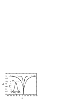
Figure 1: Similarity function of the coupled delay maps Eq. (23) without noise, $A_{xx}=A_{yy}=A_{xy}=0.$ The parameters are, $n_{0}=15,$ $b=3,$ and $a=0.975$ (squares) and $a=0.9$ (circles). The lines correspond to the fitting Eq. (14) joint with the mapping Eq. (17) [with $\delta t=1],$ indistinguishable from Eq. (21). The inset corresponds to the stationary probability distribution $P(x)$ of the process $x_{n}$ (with $a=0.9$).

In Fig. 1 we show the similarity function when the external noises are absent, i.e., the similarity corresponding to the deterministic map. In agreement with this condition, we notice that $S_{n_{0}}=0,$ implying that the manifold $x_{m+n_{0}}=y_{m}$ characterizes the asymptotic behavior. Furthermore, we find that both the expression for the continuous time case [Eq. (13) with the mapping Eq. (17)], as well as the similarity function of the map [Eq. (21)] are indistinguishable from each other (in the scale of the graphic) and both correctly fit the numerical behavior. In the inset, we show the stationary probability distribution of the master process $x_{n}.$ In agreement with our considerations, this distribution can be fit with a Gaussian distribution. From its width, and by using Eq. (19) [or Eq. (12)] we estimated the value of the chaotic force amplitude, $A\approx 3.5.$

In the absence of the noises, we corroborate that by taking the function $f[x]=\sin(x+\phi),$ independently of the value of the phase $\phi,$ the same statistical behaviors follow. This result confirms the arguments presented in the previous section [Eq. (2)] about the statistical invariance of the chaotic force under a shift of its argument.

In Fig. 2 we show the similarity function when the master and slave dynamics are affected by two uncorrelated external noises. As expected, we found that $S_{n_{0}}>0$ $(n_{0}=15).$ In the inset, we show a characteristic master-slave realization. Even in the presence of the external noises, both trajectories are approximately the same (the slave anticipate the master trajectory).

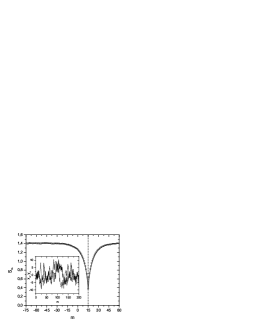
Figure 2: Similarity function of the coupled delay maps Eq. (23) subject to external Gaussian noise fluctuations. The parameters are $n_{0}=15,$ $a=0.9,$ and $b=3.$ The noise parameters are $A_{xx}=A_{yy}=0.25$ and $A_{xy}=0.$ The line corresponds to the fitting Eq. (14) joint with the mapping Eq. (17) [with $\delta t=1],$ indistinguishable from Eq. (21). The chaotic noise amplitude results $A\approx 3.5.$ The inset corresponds to a master ($x_{n},$ full line) and slave ($y_{n},$ dotted line) realization.

In contrast with the previous figure, here the fitting to the similarity function depends explicitly on the chaotic force amplitude $A.$ We found that the value of $A$ that provides the best fitting is consistent with the one found for the deterministic map (Fig. 1), i.e., $A\approx 3.5.$ Then, in this case, the inequality $A\gg\{A_{xx},A_{yy}\}$ is satisfied, implying that the fluctuations induced by the determinist chaotic dynamic are much larger than those induced by the external noise sources.

Maintaining all the parameter values corresponding to Fig. 2, we analyzed the case $A_{xx}=A_{yy}=A_{xy}.$ In this situation, the noises that drive the master and slave dynamics are exactly the same, i.e., Eq. (23) with $\xi_{n}^{x}=\xi_{n}^{y}$ (as in the continuous time case, this property follows by diagonalizing the matrix of diffusion noise coefficients $\{\{A_{xx},A_{xy}\},\{A_{xy},A_{yy}\}\}$). We found that the similarity function is almost indistinguishable from that of Fig. 2. Independently of the external noise correlations, in both cases our approach provides a very good fitting of the numerical results.

In Fig. 3, by maintaining the parameters of the deterministic map, i.e., $(a,b,n_{0}),$ we increased the amplitude of the external noises, such that $\{A_{xx},A_{yy}\}\approx A.$ Then, the external noise-induced fluctuations are of the same order as the intrinsic chaotic dynamical fluctuations. Even in this limit, our approach provides an excellent fitting of the numerical results. Both, the case of uncorrelated noises ($A_{xy}=0$ with $A_{xx}=A_{yy}$) and the case of completely correlated noises ($A_{xx}=A_{yy}=A_{xy}$) are considered. In both situations, since the external noise amplitudes are larger than in Fig. 2, the value of $S_{n_{0}}$ increases, indicating a weaker (anticipated) synchronization between the master and slave dynamics.

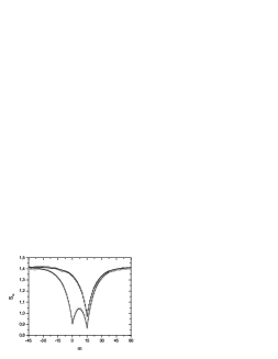
Figure 3: Similarity function of the coupled delay maps Eq. (23) driven by different noises. The circles correspond to $A_{xx}=A_{yy}=3.5$ and $A_{xy}=0,$ while the squares correspond to $A_{xx}=A_{yy}=A_{xy}=3.5.$ The parameters of the map are the same than in Fig. 2. The lines correspond to the fitting Eq. (14) joint with the mapping Eq. (17) [with $\delta t=1],$ indistinguishable from Eq. (21). The chaotic noise amplitude results $A\approx 4.3.$

In the case of completely correlated noises, $A_{xx}=A_{yy}=A_{xy},$ the similarity function develop two (local) minima, one at $m=n_{0}$ and other at $m=0.$ This feature follows from the competition between two different synchronizing mechanisms, induced by the chaotic dynamics and the external noises, respectively. In fact, as the noise that drives the master and slave dynamics is the same, its action tends to synchronize both dynamics without any time shift [see Eq. (23) with $\xi_{n}^{x}=\xi_{n}^{y}$], producing the dip at $m=0.$ In agreement with this argument, from Eq. (21) [or equivalently Eq. (13)] one can deduce that only one minimum at $m=0$ will be appreciable in the similarity function when $A\ll A_{xx}=A_{yy}=A_{xy},$ i.e., in the limit of high noise intensity.

As in Fig. 2, the similarity function depends on the amplitude $A$ of the chaotic force. Here, the best fitting to the similarity function is obtained with $A\approx 4.3.$ This value is larger than the one associated to the deterministic dynamics [Fig. 1] or the case of weak external noises [Fig. 2]. Then, in general it is necessary to consider that the chaotic force amplitude $A$ is also a function of the external noise intensities, $A=A[\{f(x),b\},A_{xx},A_{yy})].$ We remark that in concordance with the Langevin representation, the value of $A$ determined from Eqs. (19) to (21) is the same. By using the parameters of Fig. 3, we found a moderate dependence on the external noise intensities, i.e., the maximal variation of $A$ with the amplitude of the noises does not exceeds thirty percent (30%) of the deterministic map value (Fig. 1, $A\approx 3.5$). The dependence is smooth but non-monotonous. We found that $A$ saturates to a fixed value ($A\approx 4.5$) when increasing the external noise amplitudes, $A<\{A_{xx},A_{yy}\}.$

III.3 Chaotic force with a non-null average value

Our previous theoretical calculations rely on the assumption that the average (over realizations or its stationary time average) of the chaotic force is zero, i.e., $\overline{f[x(t)]}=0.$ When the dynamic, that does not include the non-linear contribution, is purely dissipative [Eq. (1) with $f(x)\rightarrow 0],$ the validity of this assumption requires that $f(x)$ takes symmetrically positive and negative values. Functions that do not satisfy this property also arise in real experimental setups hanna ; porte ; colet . In these cases, due to the pure dissipative nature of the evolution Eq. (8) [or Eq. (16)], in the long time limit the master-slave realizations will fluctuate around a non-null fixed value.

This situation can be managed by writing $f(x)=[f(x)-\overline{f(x)}]+\overline{f(x)}.$ Then, the previous theoretical calculations can be easily extended by replacing $[f(x)-\overline{f(x)}]\rightarrow\eta(t)$ [with $\overline{\eta(t)}=0$] and by maintaining the extra contribution $\overline{f(x)}$ in the final Langevin representation. For example, taking the functions $f(x)=\sin^{2}(x)$ or $f(x)=\cos^{2}(x)$ in Eq. (8), from the Langevin representation Eq. (11), it is possible to deduce that in the fully-developed chaos regime the master-slave realizations will fluctuate around $\beta/(2\gamma).$

When the dynamic without the non-linear contribution can by itself induce symmetric dynamical oscillations, the symmetry requirement on the function $f(x)$ may be eliminated [see Sec. V].

IV Effect of parameters mismatch in a hyperchaotic communication scheme

Hyperchaotic delay dynamics may be used as a resource for secure encoded communication. Different schemes have been proposed, in all the cases, it is argued that the security of the communication channel may be improved by increasing the dimension of the hyperchaotic attractor. Here, we study the dynamics porte

$$\dot{x}(t) = -\gamma x(t)+\beta f[x(t-T)]+\mathfrak{M}(t),$$ (24a)

$$\dot{y}(t) = -\gamma^{\prime}y(t)+\beta^{\prime}f[x(t-T^{\prime})].$$ (24b)

The variable $$x(t) \mathfrak{M}(t) \mathfrak{M}(t)=[d\mathfrak{m}(t)/dt+\gamma\mathfrak{m}(t)], \mathfrak{m}(t) y(t) x(t)-y(t)=\mathfrak{m}(t) x(t) \gamma^{\prime}=\gamma, \beta^{\prime}=\beta, T^{\prime}=T$$ is the carrier signal where the message is encoded. The external feed is defined by where is the message to be transmitted. The variable is the receiver. It is easy to demonstrate that in the stationary regime the state is reached, implying that the receiver is able to unmask the message encoded in the hyperchaotic dynamics of . This condition is only satisfied when the characteristic parameters of the transmitter and receiver evolutions [Eq. (24)] are the same, i.e., and nota . In any real experimental situation, it is expected that this condition is not fulfilled, i.e., the decodification of the message is performed in the presence of an unavoidable (finite) parameter mismatching. For simplicity, in the present section we will not consider the action of any external noise perturbation source.

In order to achieve a general characterization of the influence of the parameters mismatch, we take $\mathfrak{M}(t)=0.$ As in the previous section, we will use the similarity function $S(\tau)$ [Eq. (10)] as a measure of the degree of synchronization between the emitter and receiver variables.

When the transmitter dynamics is in the fully-developed chaos regime, we can extend the Langevin approach to the present situation. In order to estimate the similarity function, we replace the chaotic coupled evolution Eq. (24) by the Langevin equations

$$\dot{x}(t) = -\gamma x(t)+\eta(t-T),$$ (25a)

$$\dot{y}(t) = -\gamma^{\prime}y(t)+\sqrt{\alpha}\eta(t-T^{\prime}),$$ (25b)

where the parameter $$\alpha$$ is defined by

$$\alpha\equiv\left(\frac{\beta^{\prime}}{\beta}\right)^{2}.$$ (26)

As before, the noise $\eta(t)$ is characterized by $\overline{\eta(t)}=0,$ and $\overline{\eta(t)\eta(t^{\prime})}=\mathcal{A}\delta(t-t^{\prime})$ [Eq. (6)]. The similarity function $S(\tau)$ associated to Eq. (25), can be determine analytically by a straightforward calculation. We get

$$S(\tau)=\left[\sqrt{\frac{\gamma^{\prime}}{\alpha\gamma}}+\sqrt{\frac{\alpha\gamma}{\gamma^{\prime}}}-\frac{4\sqrt{\gamma\gamma^{\prime}}}{(\gamma+\gamma^{\prime})}\exp[-\bar{\gamma}|\tau-\Delta|]\right]^{1/2},$$ (27)

where we have defined the delay time mismatch

$$\Delta\equiv T-T^{\prime},$$ (28)

and the rate $\bar{\gamma}$ is defined as

$$\bar{\gamma}\equiv\left\{\begin{array}[]{c}\gamma\ \ \ for\ \ \ \tau>\Delta\\ \gamma^{\prime}\ \ \ for\ \ \ \tau<\Delta\end{array}\right..$$ (29)

We notice that due to the normalization constants in the definition of the similarity function Eq. (10), the final expression Eq. (27) does not depend explicitly on the chaotic force amplitude $\mathcal{A}$. The similarity function only satisfies $S(0)=0,$ when the transmitter-receiver parameters are exactly the same. In this situation, the manifold $x(t)=y(t)$ characterize the stationary regime.

IV.1 Parameter mismatch in discrete delay maps

The previous results can be extended to the coupled maps obtained from the evolution Eq. (24) after a first order Euler integration, i.e.,

$$x_{n+1} = ax_{n}+bf(x_{n-n_{0}}),$$ (30a)

$$y_{n+1} = a^{\prime}y_{n}+b^{\prime}f(x_{n-n_{0}^{\prime}}).$$ (30b)

Here, the transmitter and receiver parameters of both, the continuous and the discrete time evolutions, must be related as

$$\gamma = \frac{1-a}{\delta t},\ \ \ \ \beta=\frac{b}{\delta t},\ \ \ \ T=n_{0}\delta t,$$ (31a)

$$\gamma^{\prime} = \frac{1-a^{\prime}}{\delta t},\ \ \ \ \beta^{\prime}=\frac{b^{\prime}}{\delta t},\ \ \ \ T^{\prime}=n_{0}^{\prime}\delta t,$$ (31b)

where $$\delta t$$ is the characteristic discretization time step. For the discrete maps, the similarity function Eq. (18) reads

$$S_{m} = \left[\sqrt{\frac{(1-a^{\prime 2})}{\alpha(1-a^{2})}}+\sqrt{\frac{\alpha(1-a^{2})}{(1-a^{\prime 2})}}\right.$$ (32)

$$\left.-\frac{2\sqrt{(1-a^{2})(1-a^{\prime 2})}}{(1-aa^{\prime})}\bar{a}^{|m-m_{0}|}\right]^{1/2},$$

where we have defined

$$m_{0}\equiv n_{0}-n_{0}^{\prime},\ \ \ \ \ \ \ \ \alpha=\left(\frac{b^{\prime}}{b}\right)^{2},$$ (33)

and the “dissipative rate”

$$\bar{a}\equiv\left\{\begin{array}[]{c}a\ \ \ for\ \ \ m>m_{0}\\ a^{\prime}\ \ \ for\ \ \ m<m_{0}\end{array}\right..$$ (34)

Notice that under the mapping Eq. (31), the definition of the parameter $\alpha$ in Eq. (33) is consistent with Eq. (26).

IV.2 Numerical results

Here we consider the coupled chaotic maps

$$x_{n+1} = ax_{n}+b\cos(x_{n-n_{0}}),$$ (35a)

$$y_{n+1} = a^{\prime}y_{n}+b^{\prime}\cos(x_{n-n_{0}^{\prime}}).$$ (35b)

In the inset of Fig. 4, we show a characteristic realization of the emitter and receiver variables. By averaging over different realizations $$(\approx 10^{4}), S_{m} m_{0}=-5. b b^{\prime},$$ we get the similarity function. We notice that due to the specific values of the characteristic parameters, the receiver “synchronizes” with the “past” of the transmitter variable. In fact, attains it minimal value at Furthermore, due to the difference in the parameters and the amplitude of the receiver fluctuations are bigger than those of the transmitter.

In contrast with Fig. 2, here the similarity function is not symmetrical around its minimal value. This asymmetry has its origin in the mismatch between the “dissipative rate” parameters $a$ and $a^{\prime}.$

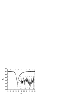
Figure 4: Similarity function of the coupled delay maps Eq. (35) (circles). The parameters are $n_{0}=15,$ $a=0.9,$ $b=3$ and $n_{0}^{\prime}=20,$ $a^{\prime}=0.8,$ $b^{\prime}=5.$ The line corresponds to the fitting Eq. (27) joint with the mapping Eq. (31) [with $\delta t=1]$, indistinguishable from Eq. (32). The inset corresponds to a realization of $x_{n}$ (full line), and $y_{n}$ (dotted line).

Clearly, the Langevin approach provides a very well fitting to the numerical simulations. Furthermore, it allows to characterize the influence of the parameters mismatch on the synchronization of the transmitter and receiver variables. The analytical quantification of this effect can be obtained from the similarity function Eq. (27) [or Eq. (32)] evaluated at the origin

$$S(0)=\left[\sqrt{\frac{\gamma^{\prime}}{\alpha\gamma}}+\sqrt{\frac{\alpha\gamma}{\gamma^{\prime}}}-\frac{4\sqrt{\gamma\gamma^{\prime}}}{(\gamma+\gamma^{\prime})}\exp[-\bar{\gamma}|\Delta|]\right]^{1/2}.$$ (36)

By a direct inspection of this expression, we realize that the dependence of $S(0)$ on the prime parameters is non-monotonous, $S(0)$ develops different minima when varying the receiver parameters. In agreement with the results of Ref. colet , assuming that it is possible to adjust a given receiver parameter, the previous expression allows us to choose the best value that maximizes the synchronization phenomenon.

V Synchronization of second-order non-linear delay differential equations

In the previous sections, we analyzed the phenomenon of chaotic synchronization for dynamics generated by first order delay equations. Nevertheless, second order delay differential equations also arise in the in the description of real experimental setups. By second order we mean equations whose linear dynamical contributions are equivalent to second order (time) derivative evolutions. Here, we demonstrate that the Langevin approach also works in that case.

Following Ref. colet we consider the evolution

$$x(t)\!+\!\frac{\dot{x}(t)}{\gamma}\!+\!\frac{1}{\theta}\!\int_{0}^{t}\!x(s)ds\! = \!\beta\!\cos^{2}[x(t-T)]\!+\!\xi_{x}(t),$$ (37)

$$y(t)\!+\!\frac{\dot{y}(t)}{\gamma^{\prime}}\!+\!\frac{1}{\theta^{\prime}}\!\int_{0}^{t}\!y(s)ds\! = \!\beta^{\prime}\!\cos^{2}[x(t-T^{\prime})]\!+\!\xi_{y}(t),\ \ \ \ \$$ (38)

which describe synchronization in a set of coupled electro-optical laser devices. The integral contributions proportional to $(1/\theta)$ and $(1/\theta^{\prime})$ indicate that the linear evolutions defined by the left hand side of Eqs. (37) and (38) are equivalent to a set of second order derivative differential equations. In addition to the parameters mismatch, we also consider the action of external additive noises $\xi_{x}(t)$ and $\xi_{y}(t)$, whose mutual and self-correlations are defined by Eq. (9). In order to simplify the final expression here we not consider any mismatch in the phase of the chaotic forces nota .

Under the same conditions than in the previous sections, we assume that $x(t)$ and $y(t),$ in the long time limit, attain the fully-developed chaos regime, allowing us to replace the nonlinear delay forces by noise contributions with the same time arguments, delivering

$$x(t)\!+\!\frac{\dot{x}(t)}{\gamma}\!+\!\frac{1}{\theta}\int_{0}^{t}x(s)ds\! = \!\eta(t-T)\!+\!\xi_{x}(t),$$ (39a)

$$y(t)\!+\!\frac{\dot{y}(t)}{\gamma^{\prime}}\!+\!\frac{1}{\theta^{\prime}}\int_{0}^{t}y(s)ds\! = \!\sqrt{\alpha}\eta(t-T^{\prime})\!+\!\xi_{y}(t),\ \ \ \ \ \ \$$ (39b)

where as before, $$\alpha=(\beta^{\prime}/\beta)^{2}. \eta(t) \overline{\eta(t)}=0. \cos^{2}[x] \{\theta,\theta^{\prime}\}<\infty, \theta=\theta^{\prime}=\infty.$$ The correlation of is again defined by Eq. (6), and we take Notice that in spite that the nonlinear contribution is always positive, when the second order linear evolution introduces self dynamical oscillations that imply that its effective action averaged over realizations (or its stationary time average) must be taken as zero. This property breaks down when the integral contributions are absent, i.e., in the limit

The Green functions associated to the linear evolutions Eq. (39) can be obtained straightforwardly in the Laplace domain, being defined by the addition of two exponential functions. After integrating formally both equations for each realization of the noises, it follow

$$\lim_{t\rightarrow\infty}\langle\overline{x^{2}(t)}\rangle = \frac{\gamma}{2}(\mathcal{A}+\mathcal{A}_{xx}),$$ (40a)

$$\lim_{t\rightarrow\infty}\langle\overline{y^{2}(t)}\rangle = \frac{\gamma^{\prime}}{2}(\alpha\mathcal{A}+\mathcal{A}_{yy}).$$ (40b)

The similarity function [Eq. (10)] reads

$$S(\tau)=\left\{\frac{\sqrt{\frac{\gamma}{\alpha\gamma^{\prime}}}\left(1+\frac{\mathcal{A}_{xx}}{\mathcal{A}}\right)+\sqrt{\frac{\alpha\gamma^{\prime}}{\gamma}}\left(1+\frac{\mathcal{A}_{yy}}{\alpha\mathcal{A}}\right)-4\mu\left[\Xi(\tau-\Delta)+\frac{\mathcal{A}_{xy}}{\sqrt{\alpha}\mathcal{A}}\Xi(\tau)\right]}{\left(1+\frac{\mathcal{A}_{xx}}{\mathcal{A}}\right)^{1/2}\left(1+\frac{\mathcal{A}_{yy}}{\alpha\mathcal{A}}\right)^{1/2}}\right\}^{1/2}.$$ (41)

Here, $\Delta=T-T^{\prime}.$ The function $\Xi(t)$ is defined as

$$\Xi(t)=e^{-\frac{1}{2}\bar{\gamma}|t|}\left[\cosh(\bar{\Phi}|t|/2)-\bar{\nu}\frac{\bar{\gamma}}{\bar{\Phi}}\sinh(\bar{\Phi}|t|/2)\right],$$ (42)

where the dissipative rate $\bar{\gamma}$ is defined by

$$\bar{\gamma}\equiv\left\{\begin{array}[]{c}\gamma\ \ \ if\ \ \ t>0\\ \gamma^{\prime}\ \ \ if\ \ \ t<0\end{array}\right..$$ (43)

For $t>0,$ the frequency $\bar{\Phi}$ reads

$$\bar{\Phi}\equiv\gamma\sqrt{1-\frac{4}{\theta\gamma}},\ \ \ \ \ \ if\ \ \ t>0,$$ (44)

while the dimensionless parameter $\bar{\nu}$ is

$$\bar{\nu}\equiv 1-\frac{2}{\theta(\theta+\theta^{\prime})}\left(\frac{\theta}{\gamma}-\frac{\theta^{\prime}}{\gamma^{\prime}}\right),\ \ \ \ \ \ if\ \ \ t>0.$$ (45)

For $t<0,$ both $\Phi$ and $\nu$ are defined by interchanging $\theta\leftrightarrow\theta^{\prime}$ and $\gamma\leftrightarrow\gamma^{\prime}$ in the previous expressions. Finally, in Eq. (41), we have also defined the dimensionless parameter

$$\mu\equiv\frac{\sqrt{\gamma\gamma^{\prime}}(\theta+\theta^{\prime})}{(\theta\gamma^{\prime}/\theta^{\prime}\gamma)+[(\theta+\theta^{\prime})(\gamma+\gamma^{\prime})-2]+(\theta^{\prime}\gamma/\gamma^{\prime}\theta)},$$ (46)

which is symmetric in the emitter and receiver parameters.

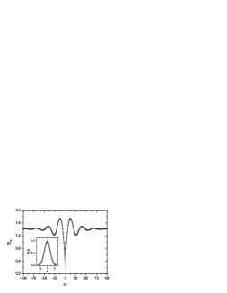
Figure 5: Similarity function of the coupled delay maps Eq. (47) (circles) without noises, $A_{xx}=A_{yy}=A_{xy}=0$ and without mismatching, $n_{0}^{\prime}=n_{0},$ $a^{\prime}=a,$ $b^{\prime}=b$ and $\omega^{\prime}=\omega.$ The parameters are $n_{0}=20,$ $a=0.9,$ $b=3$ and $\omega=0.05.$ The line corresponds to the fitting Eq. (41) under the mapping Eq. (48) [with $\delta t=1].$ The inset corresponds to the stationary probability distribution of the process $x_{n}.$

In order to check the validity of the previous approach, we consider the discrete maps associated to Eqs. (37) and (38) by Euler integration

$$x_{n+1} = ax_{n}-\omega\sum_{j=0}^{n}x_{j}+b\cos^{2}(x_{n-n_{0}})+\xi_{n}^{x},$$ (47a)

$$y_{n+1} = a^{\prime}y_{n}-\omega^{\prime}\sum_{j=0}^{n}y_{j}+b^{\prime}\cos^{2}(x_{n-n_{0}^{\prime}})+\xi_{n}^{y}.\ \ \ \ \$$ (47b)

The (transmitter) parameters mapping reads

$$\gamma=\frac{(1-a)}{\delta t},\ \ \ \ \ \ \ \theta=\delta t\frac{(1-a)}{\omega},\ \ \ \ \ \ \ \beta=\frac{b}{(1-a)}.$$ (48)

The same relations are valid for the prime (receiver) parameters. The noises $\xi_{n}^{x}$ and $\xi_{n}^{y},$ joint with the corresponding mapping for their amplitudes are defined below Eq. (16). The chaotic force amplitude of the continuous and discrete time evolutions are related by $\mathcal{A}=A/\delta t.$

In Fig. 5 we plot the similarity function [Eq. (18)] associated to the coupled maps Eq. (47) in absence of parameters mismatch and without the external noises. The analytical result Eq. (41), under the mapping Eq. (48), provides an excellent fitting of the numerical results. In contrast with the previous sections (see for example Fig. 1), here the similarity function develops an oscillatory behavior, its origin can be associated to the integral contributions in the dissipative dynamics of Eqs. (37) and (38). Their characteristic frequency follows from Eq. (44).

In order to check the achievement of the fully-developed chaos regime kilom , in the inset we show the stationary probability distribution of $x_{n}.$ Consistently, this distribution can be fitted with a Gaussian distribution.

In Fig. 6, for other set of characteristic parameters, we plot the similarity function in presence of parameter mismatch and external noise sources. As in the previous case, the fitting Eq. (41) correctly match the numerical results. The effective chaotic force amplitude is $A\approx 1.2.$ The asymmetry of $S_{m}$ around its minimum value follows from the parameter mismatch between the evolution of $x_{n}$ and $y_{n}.$

In the inset, maintaining the parameters corresponding to the evolution of $x_{n},$ we plot the similarity function in absence of both, parameters mismatch and the external noise contributions. In this case, the chaotic force amplitude [determine from Eq. (40)] is $A\approx 1.$

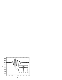
Figure 6: Similarity function of the coupled delay maps Eq. (47) (circles) with parameters mismatch and under the action of external noises. The parameters are $n_{0}=20,$ $a=0.98,$ $b=3,$ $\omega=0.01,$ and $n_{0}^{\prime}=22,$ $a^{\prime}=0.95,$ $b^{\prime}=4,$ $\omega^{\prime}=0.0125.$ The noise parameters are $A_{xx}=A_{yy}=0.0225$ and $A_{xy}=0.$ The line corresponds to the fitting Eq. (41) joint with the mapping Eq. (48) [with $\delta t=1].$ The inset corresponds to the similarity function in absence of noises and without mismatching.

As in the previous section, a remarkable aspect of our analytical results is that they allows us to know the influence of different realistic effects on the chaotic synchronized manifold. For example, for a given set of fixed parameters, which may include the amplitude of the external noises, one can determine the value of the rest of the parameters that minimizes the similarity function at $\tau=0,$ giving rise to a maximization in the degree of synchronization between the emitter and receiver variables. This kind of analysis follows straightforwardly from our analytical results.

VI Conclusions

In this paper, we have characterized the phenomenon of chaotic synchronization in scalar coupled non-linear time delay dynamics. Our formalism relies in recognizing that in a fully-developed chaos regime, the trajectories associated to a broad class of hyperchaotic attractors are statistically equivalent to the realizations of a linear Langevin equation. This equivalence can be established when the function that defines the driven chaotic delay force is an oscillatory one, such that its dynamical action can be represented by a delta-correlated noise. Given this Langevin representation, the coupled nonlinear delay evolutions, where the phenomenon of chaotic synchronization happens, are replaced by a set of linear stochastic equations where the noise that represents the chaotic force maintains the corresponding time arguments. The statistical properties of the Langevin equations can be obtained analytically, providing an excellent estimation of the stationary statistical properties of the synchronized manifold.

Using the Langevin representation, we analyzed the phenomenon of anticipated synchronization in the presence of external additive noises. We also characterized the effect of parameters mismatch in a hyperchaotic communication scheme. Second-order delay equations associated to an electro optical device were also characterized. The analytical predictions of the Langevin approach correctly fit numerical simulations in discrete coupled nonlinear delay maps associated to the corresponding continuous time evolutions.

In all cases, the degree of synchronization (between the master-slave or emitter-receiver variables) was characterized through a similarity function, defined in terms of the correlation between the synchronizing systems. When the departure from perfect synchronization is due to a parameter mismatching, the fitting to the similarity function does not involve any free parameter. When the action of external noises is considered the fitting depends on the effective chaotic force amplitude.

Our results are interesting from both, theoretical and experimental point of view. From our analytical expressions it is possible to evaluate under which conditions a given undesired effect can be minimized by controlling the rest of the parameters. On the other hand, in the context of hyperchaotic communication schemes, while high dimensional systems increase the complexity of the masking signals, our results show that the corresponding statistical properties may adopt a simple analytical form. In fact, by measuring the similarity function our results allow to infer the value of some of the characteristic parameters of the hyperchaotic delay dynamics.

The present study may be continued in different relevant directions such as the extension of the Langevin representation beyond the fully-developed chaos regime (non-Gaussian chaos) as well as for non-scalar chaotic dynamics. Furthermore, the characterization of the dependence of the effective chaotic force amplitude with the external noise parameters is an open interesting issue.

References

- (1) A. Pikovsky, M. Rosenblum, and J. Kurths, Synchronization, A universal concept in nonlinear sciences, Cambridge Nonlinear Science Series 12, (2001).
- (2) H. Fujisaka and T. Yamada, Prog. Theor. Phys. 69, 32 (1983); ibid, 75, 1087 (1986).
- (3) A.S. Pikovsky, Radiophys. Quant. Electron. 27, 576 (1984).
- (4) A.S. Pikovsky, Sov. J. Commun. Technol. Electron 30, 85 (1985).
- (5) A.S. Pikovsky and P. Grassberger, J. Phys. A 24, 4587 (1991).
- (6) L.M. Pecora and T.L. Carroll, Phys. Rev. Lett. 64, 821 (1990).
- (7) L.M. Pecora and T.L. Carroll, Phys. Rev. A 44, 2374 (1991).
- (8) O.E. Rossler, Phys. Lett. A 71, 155 (1979).
- (9) L. Kocarev and L. Parlitz, Phys. Rev. Lett. 74, 5028 (1995).
- (10) J.H. Peng, E.J. Ding, M. Ding, and W. Yang, Phys. Rev. Lett. 76, 904 (1996).
- (11) Y.C. Lai, Phys. Rev. E 55, 4861(R) (1997).
- (12) M.K. Ali and J.Q. Fang, Phys. Rev. E 55, 5285 (1997).
- (13) K.M. Short and A.T. Parker, Phys. Rev. E 58, 1159 (1998).
- (14) M.C. Mackey and L. Glass, Science 197, 287 (1977).
- (15) J. Foss, A. Longtin, B. Mensour, and J. Milton, Phys. Rev. 76, 708 (1996).
- (16) N. MacDonald, Biological Delay Systems: Linear Stability Theory (Cambridge University Press, Cambridge, England, 1989).
- (17) P.K. Asea and P.J. Zak, J. Econ. Dyn. Control 23, 1155 (1999); M.C. Mackey, J. Econ. Theory 48, 497 (1989).
- (18) K. Ikeda, H. Daido, O. Akimoto, Phys. Rev. Lett. 45, 709 (1980).
- (19) K. Ikeda and K. Matsumoto, Phys. D 29, 223 (1987).
- (20) F. Arecchi, W. Gadomski, and R. Meucci, Phys. Rev. A 34, 1617 (1993).
- (21) L. Larger, P.A. Lacourt, S. Poinsot, and M. Hanna, Phys. Rev. Lett. 95, 043903 (2005).
- (22) M. Le Berre, E. Ressayre, A. Tallet, and H.M. Gibbs, Phys. Rev. Lett. 56, 274 (1986).
- (23) J.D. Farmer, Physica D 4, 366 (1982).
- (24) P. Grassberger and I. Procaccia, Physica D 9, 189 (1983).
- (25) M. Le Berre, E. Ressayre, A. Tallet, H.M. Gibbs, D.L. Kaplan, and M.H. Rose, Phys. Rev. A 35, 4020(R) (1987).
- (26) J.P. Goedgebuer, L. Larger, and H. Porte, Phys. Rev. Lett. 80, 2249 (1998).
- (27) C. Zhou and C.H. Lai, Phys. Rev. E 60, 320 (1999).
- (28) L. Yaowen, G. Guangming, Z. Hong, and W. Yinghai, Phys. Rev. E 62, 7898 (2000).
- (29) V.S. Udaltsov, J.P. Goedgebuer, L. Larger, and W.T. Rhodes, Phys. Rev. Lett. 86, 1892 (2001).
- (30) H.U. Voss, Phys. Rev. E 61, 5115 (2000); ibid, 64, 039904 (2000).
- (31) H.U. Voss, Phys. Rev. Lett. 87, 014102 (2001).
- (32) H.U. Voss, Phys. Lett. A 279, 207 (2001).
- (33) K. Pyragas, Phys. Rev. E 58, 3067 (1998).
- (34) C. Masoller, Phys. Rev. Lett. 86, 2782 (2001).
- (35) C. Masoller and D.H. Zanette, Phys. A 300, 359 (2001).
- (36) S. Sivaprakasam, E.M. Shahverdiev, P.S. Spencer, and K.A. Shore, Phys. Rev. Lett. 87, 154101 (2001).
- (37) T. Heil, I. Fischer, W. Elsässer, J. Mulet, and C.R. Mirasso, Phys. Rev. Lett. 86, 795 (2001).
- (38) E. Hernandez-Garcia, C. Masoller, and C.R. Mirasso, Phys. Lett. A 295, 39 (2002).
- (39) M. Ciszak, O. Calvo, C. Masoller, C.R. Mirasso, and R. Toral, Phys. Rev. Lett. 90, 204102 (2003).
- (40) S. Tang and J.M. Liu, Phys. Rev. Lett. 90, 194101 (2003).
- (41) D.J. Gauthier and J.C. Bienfang, Phys. Rev. Lett. 77, 1751 (1996).
- (42) G.A. Johnson, D.J. Mar, T.L. Carroll, and L.M. Pecora, Phys. Rev. Lett. 80, 3956 (1998).
- (43) Y.C. Kouomou and P. Colet, Phys. Rev. E 69, 056226 (2004).
- (44) R. Brown, N.F. Rulkov, and N.B. Tufillaro, Phys. Rev. E 50, 4488 (1994).
- (45) W. Lin and Y. He, Chaos 15, 023705 (2005).
- (46) G. Györgyi and P. Szépfalusy, J. Stat. Phys. 34, 451 (1983).
- (47) B. Dorizzi, B. Grammaticos, M. Le Berre, Y. Pomeau, E. Ressayre, and A. Tallet, Phys. Rev. A 35, 328 (1987).
- (48) M. Le Berre, E. Ressayre, A. Tallet, and Y. Pomeau, Phys. Rev. A 41, 6635 (1990).
- (49) M.G. Rosenblum, A.S. Pikovsky, and J. Kurths, Phys. Rev. Lett. 78, 4193 (1997).
- (50) There exist cases where this condition is not satisfied, as for example for the Mackey-Glass dynamic mackey ; berre1 , which arise in the context of white-blood-cell production.
- (51) N.G. van Kampen, in Stochastic Processes in Physics and Chemistry, Second Edition, North-Holland, Amsterdam, (1992).
- (52) Strictly, the mapping defined by Eqs. (4) and (5) is sufficient for Markovian Gaussian process. The Markovian property is guaranteed by the validity of the white noise approximation Eq. (6). On the other hand, we notice that independently of the probability distribution associated to by appealing to the central limit theorem kampen , the correlation Eq. (6) guarantees that, in the long time regime, Eq. (3) always converges to a Gaussian process.
- (53) It is also possible to consider extra parameters mismatch in the transmitter-receiver nonlinearities, as for example the phase in colet . This case can be worked out in the Langevin representation in a similar way by discomposing the function in two shiftless terms and considering their respective symmetries properties. For simplicity, we will not consider this case.
- (54) Taking the experimental parameters of Ref. colet , the dynamics goes beyond the Gaussian chaos regime. Our formalism may also be used as an estimator of the statistical properties in this regime. Nevertheless, the quality of the fitting departs from that showed in the figures of this paper. On the other hand, from Eq. (39), it is possible to write the Fourier transform () of as and a similar one for Then, the band-pass filter approximation introduced in Ref. colet can be read as a rough approximation to these expressions.