Multiple magnetic barriers in graphene

Abstract

We study the behavior of charge carriers in graphene in inhomogeneous perpendicular magnetic fields. We consider two types of one-dimensional magnetic profiles, uniform in one direction: a sequence of $N$ magnetic barriers, and a sequence of alternating magnetic barriers and wells. In both cases, we compute the transmission coefficient of the magnetic structure by means of the transfer matrix formalism, and the associated conductance. In the first case the structure becomes increasingly transparent upon increasing $N$ at fixed total magnetic flux. In the second case we find strong wave-vector filtering and resonant effects. We also calculate the band structure of a periodic magnetic superlattice, and find a wave-vector-dependent gap around zero-energy.

I Introduction

The electronic properties of graphenereviews in the presence of inhomogeneous perpendicular magnetic fields have very recently attracted considerable theoretical attention ale ; tarun ; cserti ; sim ; masir ; tahir ; zhai ; heinzel ; kormanios ; ghosh . In graphene the charge carriers close to the Fermi points $K$ and $K^{\prime}$ form a relativistic gas of chiral massless (Dirac-Weyl) quasiparticles with a characteristic conical spectrum. This has far-reaching consequences. For example, quasiparticles in graphene are able to tunnel through high and wide electrostatic potential barriers, a phenomenon often referred to as Klein tunneling, and related to their chiral naturekleintunn . Moreover, in a uniform magnetic field graphene exhibits an unconventional half-integer quantum Hall effect iqheexp , which can be understood in terms of the existence, among the relativistic Landau levels formed by the quasiparticles, of a zero-energy oneiqheth .

From a theoretical perspective, it is then interesting to explore how the Dirac-Weyl (DW) nature of the charge carriers affects their behavior in non-uniform magnetic fields. Such investigation has been started in Ref. ale , and here we generalize and expand on it by studying several more complex geometries.

Experimentally, inhomogeneous magnetic profiles on submicron scales in ordinary 2DEGs in semiconductor heterostructures have been produced in several ways, and magnetic barriers with heights up to 1 T have been obtained. One approach exploits the fringe field produced by ferromagnetic stripes fabricated on top of the structure heinzelex . Another possibility consists in applying a uniform magnetic field to a 2DEG with a step leadbeater . In yet another approach, a film of superconducting material with the desired pattern is deposited on top of the structure, and a uniform magnetic field is applied.bending In this way, magnetic structures with different geometries have been experimentally realized, and their mesoscopic transport properties have been studied, e.g. transport through single magnetic barriers expbar and superlattices carmona , magnetic edge states close to a magnetic step henini , and magnetically confined quantum dots or antidots antidots . Correspondingly, there exists an extensive theoretical literature, pioneered by the works of F.M. Peeters and collaborators peetersstructures , which elucidates the basic mechanisms underlying the behaviors observed in experiments.

In principle, the same concepts and technologies can be used to create similar magnetic structures in graphene, once the graphene sheet is covered by an insulating layer, which has recently been demonstrated feasible huard ; williams . Although at the time of writing there is yet no published experimental work demonstrating magnetic barriers in graphene, this should be within reach of present-day technology, which provides motivation for the present work.

In a previous paper ale we showed that, in contrast to electrostatic barriers, a single magnetic barrier in graphene totally reflects an incoming electron, provided the electron energy does not exceed a threshold value related to the total magnetic flux through the barrier. Above this threshold, the transmission coefficient strongly depends on the incidence angle ale ; masir . These observations were used to argue that charge carriers in graphene can be confined by means of magnetic barriers, which may thus provide efficient tools to control the transport properties in future graphene-based nanodevices.

Here we focus on more complex multiple barrier configurations and magnetic superlattices. We consider two types of one-dimensional profiles. In the first case the magnetic field in the barrier regions is always assumed to point upwards, while in the second it points alternatingly upwards and downwards. We shall see that there are sharp differences in the transport properties of the two cases.

The outline of the paper is the following. In Sec. II we introduce the Dirac-Weyl Hamiltonian for graphene, the two types of magnetic profiles we consider in the rest of the paper, and the transfer matrix formalism for Dirac-Weyl particles. In Sec. III and Sec. IV we compute and discuss the transmission coefficient separately for the two cases. In Sec. V we consider a periodic magnetic superlattice, and determine its band structure. Finally, in Sec. VI we summarize our results and draw our conclusions.

II Hamiltonian and transfer matrix

Electrons in clean graphene close to the two Fermi points $K$ and $K^{\prime}$ are described by two decoupled copies of the Dirac-Weyl (DW) equation. We shall focus here on a single valley and neglect the electron spin.footnote1 Including the perpendicular magnetic field via minimal coupling, the DW equation reads

$$v_{F}{\bm{\sigma}}\cdot\left(-i{\bf\hbar\nabla}+\frac{e}{c}{\bf A}\right)\Psi=E\Psi,$$ (1)

where ${\bm{\sigma}}=(\sigma_{x},\sigma_{y})$ are Pauli matrices acting in sublattice space, and $v_{F}=8\times 10^{5}\,$m/s is the Fermi velocity in graphene. In the Landau gauge, ${\bm{A}}=(0,A(x))$, with $B_{z}=\partial_{x}A$, the $y$-component of the momentum is a constant of motion, and the spinor wavefunction can be written as $\Psi(x,y)=\psi(x)e^{ik_{y}y}$, whereby Eq. (1) is reduced to a one-dimensional problem:

$$\left(\begin{array}[]{cc}-E&-i\partial_{x}-i(k_{y}+A(x))\\ -i\partial_{x}+i(k_{y}+A(x))&-E\end{array}\right)\psi=0.$$ (2)

Eq. (2) is written in dimensionless units: with $B$ the typical magnitude of the magnetic field, and $\ell_{B}=\sqrt{\hbar c/eB}$ the associated magnetic length, we express the vector potential $A(x)$ in units of $B\ell_{B}$, the energy $E$ in units of $\hbar v_{F}/\ell_{B}$, and $x$ and $k_{y}$ respectively in units of $\ell_{B}$ and $\ell^{-1}_{B}$. The values of local magnetic fields in the barrier structures produced by ferromagnetic stripes range up to 1 T, with typical values of the order of tenth of Tesla. For $B\approx 0.1\,$T, we find $\ell_{B}\approx 80\,$nm and $\hbar v_{F}/\ell_{B}\approx 7\,$meV, which set the typical length and energy scales.

Figure 1: Magnetic profile Eq. (3): $N$ magnetic barriers of width $d_{B}$ separated by nonmagnetic regions of width $d_{0}$.

We shall consider two types of magnetic field profiles. In the first case, illustrated in Fig. 1, the profile consists of a sequence of $N$ magnetic barriers of equal height $B$ (assumed positive for definiteness) and width $d_{B}$, separated by nonmagnetic regions of width $d_{0}$. The vector potential is then chosen as

$$A(x)=\left\{\begin{array}[]{ll}0,&\;\;x\in[-\infty,0],\\ nd_{B}+(x-x_{n}),&\;\;x\in[x_{n},x_{n}+d_{B}],\\ (n+1)d_{B},&\;\;x\in[x_{n}+d_{B},x_{n+1}],\\ Nd_{B},&\;\;x\in[x_{N},\infty],\end{array}\right.$$ (3)

where $n=0,\dots,N-1$ and $x_{n}=n(d_{0}+d_{B})$. The quantity $Nd_{B}$ is the total magnetic flux through the structure per unit length in the $y$-direction.footnote2 We shall refer to this profile as the multiple barriers case and discuss it in Sec. III.

Figure 2: Magnetic profile Eq. (4): $N$ magnetic barriers of width $d_{B}$ separated by magnetic wells of width $d_{-B}$.

In the second case, illustrated in Fig. 2, each magnetic barrier is followed by a region of width $d_{-B}$ of opposite magnetic field. The vector potential is accordingly chosen as

$$A(x)=\left\{\begin{array}[]{ll}0,&\;\;x\in[-\infty,0],\\ nD+(x-x_{n}),&\;\;x\in[x_{n},x_{n}+d_{B}],\\ nD+(2d_{B}+x_{n}-x),&\;\;x\in[x_{n}+d_{B},x_{n+1}],\\ ND,&\;\;x\in[x_{N},\infty],\end{array}\right.$$ (4)

where $n=0,\dots,N-1$, $x_{n}=n(d_{B}+d_{-B})$, and $D=d_{B}-d_{-B}$. We shall refer to this profile as the alternating barrier-well case, and discuss it in Sec. IV. The parameter $D$ has the meaning of net magnetic flux through a cell formed by a barrier and a well. For $D=0$ this profile can be extended to a periodic magnetic superlattice, a case considered in Sec. V.

With our gauge choice, the value of the vector potential on the right of the structure is equal to the total magnetic flux $\Phi$ through it

$$\Phi\equiv A(x>x_{N})=\left\{\begin{array}[]{ll}Nd_{B},&\quad{\text{case 1}},\\ N(d_{B}-d_{-B}),&\quad{\text{case 2}},\end{array}\right.$$ (5)

which is an important control parameter for the transport properties.

In both cases, the solutions to Eq. (2) can be obtained by first writing the general solution in each region of constant $B_{z}$ as linear combination (with complex coefficients) of the two independent elementary solutions, and then imposing the continuity of the wavefunction at the interfaces between regions of different $B_{z}$, to fix the complex coefficients. This procedure is most conveniently performed in the transfer matrix formalism. Here we directly use this approach and refer the reader to Refs.mckellar , barbier for a detailed discussion.

The transfer matrix

$$\hat{T}=\left(\begin{array}[]{cc}T_{11}&T_{12}\\ T_{21}&T_{22}\end{array}\right)$$ (6)

relates the wave function on the left side of the magnetic structure ($x<x_{0}=0$)

$$\psi(x)=\left(\begin{array}[]{l}1\\ \frac{k^{i}_{x}+ik_{y}}{E}\end{array}\right)e^{ik^{i}_{x}x}+r\left(\begin{array}[]{l}1\\ \frac{-k^{i}_{x}+ik_{y}}{E}\end{array}\right)e^{-ik^{i}_{x}x},$$ (7)

where $k^{i}_{x}=\sqrt{E^{2}-k_{y}^{2}}$, to the wave function on the right side ($x>x_{N}$)

$$\psi(x)=t\sqrt{\frac{k^{i}_{x}}{k^{f}_{x}}}\left(\begin{array}[]{c}1\\ \frac{k^{f}_{x}+i(k_{y}+\Phi)}{E}\end{array}\right)e^{ik^{f}_{x}x},$$ (8)

where $k_{x}^{f}=\sqrt{E^{2}-(k_{y}+\Phi)^{2}}$. The coefficients $r$ and $t$ are resp. the reflection and transmission amplitudes, and we used that with our gauge choices (3) and (4), the vector potential vanishes on the left of the magnetic structure, and on the right side is equal to $\Phi$. As usual, the factor $\sqrt{k^{i}_{x}/k^{f}_{x}}$ ensures proper normalization of the probability current. The relation which expresses the continuity of the wave function is then given bytransfer

$$\left(\begin{array}[]{l}1\\ r\end{array}\right)=\hat{T}\left(\begin{array}[]{l}\sqrt{k^{i}_{x}/k^{f}_{x}}\,t\\ 0\end{array}\right).$$ (9)

Solving Eq. (9) for $t$, we get the transmission probability ${\cal T}$ as

$${\cal T}(E,k_{y})=|t|^{2}=\frac{k_{x}^{f}}{k_{x}^{i}}\frac{1}{|T_{11}|^{2}}.$$ (10)

Once ${\cal T}(E,k_{y})$ is known, it is straightforward to compute the zero-temperature conductance by integrating ${\cal T}$ over one half of the (Fermi) energy surfacepeetersfilter ; masir :

$$G(E)=G_{0}\int_{-\frac{\pi}{2}}^{\frac{\pi}{2}}d\phi\,\cos\phi\,{\cal T}(E,E\sin\phi),$$ (11)

where $\phi$ is the incidence angle (we measure angles with respect to the $x$-direction), defined by $k_{y}=E\sin\phi$, and $G_{0}=2e^{2}EL_{y}/\pi h$. $L_{y}$ is the length of the graphene sample in the $y$ direction, and $G_{0}$ includes a factor $4$ coming from the spin and valley degeneracy.

Before to proceed with the calculations, we can derive a simple and general condition for a non-vanishing transmission. For this purpose it is convenient to parametrize the momenta in the leftmost and rightmost regions resp. in terms of incidence and emergence angles, $\phi$ and $\phi_{f}$:

$$k^{i}_{x} = E\cos\phi,\quad\quad k_{y}=E\sin\phi,$$ (12)

$$k^{f}_{x} = E\cos\phi_{f},\quad\quad k_{y}=E\sin\phi_{f}-\Phi.$$ (13)

The emergence angle is then fixed by the conservation of $k_{y}$:

$$\sin\phi=\sin\phi_{f}-\frac{\Phi}{E}.$$ (14)

Equation (14) implies that transmission through the structure is only possible if $\phi_{i}$ satisfies the condition

$$\left|\sin\phi+\frac{\Phi}{E}\right|\leq 1.$$ (15)

This condition, already discussed in Ref. ale for the case of a single barrier, is in fact completely general and independent of the detailed form of the magnetic field profile. It only requires that the magnetic field vanishes outside a finite region of space. For $|\Phi/E|>2$, it implies that the magnetic structure completely reflects both quasiparticles and quasiholes. As a consequence of this angular threshold, the conductance has an upper bound given by

$$G_{s}(E)\equiv G_{0}\left(2-\left|{\frac{\Phi}{E}}\right|\right)\;\theta\left(2|E|-|\Phi|\right),$$ (16)

with the Heaviside step function $\theta$. If the vector potential profile is monotonous, $G_{s}$ also coincides with the classical conductance, obtained by setting ${\cal T}=\theta(1-|\sin\phi+\Phi/E|)$. If, however, $A(x)$ is not monotonous, the classical conductance is obtained by replacing $|\Phi|$ in Eq. (16) with the maximal value of $|A|$ in the structure, since a classical particle is totally reflected as soon as $|A|_{max}$ (rather than the total flux $|\Phi|$) exceeds twice the energy.

Before moving to the next section, we notice, as an aside remark, that Eq. (2) can easily be solved in closed form for $E=0$. The zero-energy spinors are then given by

$$\psi_{+} \propto \left(\begin{array}[]{c}1\\ 0\end{array}\right)e^{k_{y}x+\int^{x}A(x^{\prime})dx^{\prime}},$$ (19)

$$\psi_{-} \propto \left(\begin{array}[]{c}0\\ 1\end{array}\right)e^{-k_{y}x-\int^{x}A(x^{\prime})dx^{\prime}}.$$ (22)

These wave functions are admissible if and only if they are normalizable, which depends on the sign of $k_{y}$ and the behavior of the magnetic field at $x\rightarrow\pm\infty$. In fact, for any $A(x)$, at most one among $\psi_{+}$ and $\psi_{-}$ is admissible. If the magnetic field vanishes outside a finite region of space, as in our case, one can always choose a gauge in which $A(x)=0$ on the left of the magnetic region and $A(x)=\Phi$ on its right. It is then straightforward to check that for $0<k_{y}<-\Phi$, the only normalizable solution is (19), whereas for $-\Phi<k_{y}<0$, the normalizable solution is (22). In particular, we find that, when the net magnetic flux through the structure vanishes, there exist no zero-energy states. This is nicely confirmed by the calculation of the spectrum of the periodic magnetic superlattice in Sec. V. The zero-energy state is a bound state localized in the structure. Additional bound states of higher energy may also occurmasir , but we do not further investigate this problem here.

III Multiple barriers

In this section we focus on the magnetic profile in Eq. (3). In order to compute the transfer matrix $\hat{T}$, we need the two elementary solutions of the DW equation (2) for $B_{z}=0$ and the two for $B_{z}=1$.

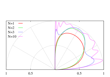
Figure 3: (Color online) Angular dependence of the transmission probability at $E=1$, through $N=1,2,3,10$ barriers of width $d_{B}=1/N$ (keeping in this way constant the flux $\Phi=Nd_{B}=1$), and spaced by $d_{0}=10$.

Figure 4: The conductance $G/G_{0}$ at $E=1$ for several values of $N$ with $d_{B}=1/N$, such that $\Phi=1$, and $d_{0}=10$ (black dots linked by long-dashed line, which is a guide to the eye only). The upper bound (dashed line) corresponds to the classical value $G_{s}/G_{0}=1$ (see Eq. (16)) while the dotted line is the curve given by Eq. (30) as a function of $N$.

We can then construct the $2\times 2$ matrices ${\cal W}_{0}(x)$ and ${\cal W}_{B}(x)$, whose columns are given by the spinor solutions. In the nonmagnetic regions we have

$${\cal W}_{0}(x)=\left(\begin{array}[]{ll}e^{ik_{x}x}&e^{-ik_{x}x}\\ \frac{k_{x}+i(k_{y}+A)}{E}e^{ik_{x}x}&\frac{-k_{x}+i(k_{y}+A)}{E}e^{-ik_{x}x}\end{array}\right),$$ (23)

where $k_{x}(x)=\sqrt{E^{2}-(k_{y}+A(x))^{2}}$. In the regions with $B_{z}=1$ we have

$${\cal W}_{B}(x)=\left(\begin{array}[]{ll}D_{p}(q)&D_{p}(-q)\\ \frac{i\sqrt{2}}{E}D_{p+1}(q)&\frac{-i\sqrt{2}}{E}D_{p+1}(-q)\end{array}\right),$$ (24)

where $q=\sqrt{2}(A(x)+k_{y})$, $p=E^{2}/2-1$, and $D_{p}(q)$ is the parabolic cylinder functiongradshtein . These matrices play the role of partial transfer matrices, and allow us to express the condition of continuity of the wave function at each interface between the nonmagnetic and the magnetic regions. After straightforward algebra, we get

$$\hat{T}=\hat{T}_{0}\,\hat{T}_{1}\,\cdots\,\hat{T}_{N-1},$$ (25)

where

$$\hat{T}_{n}={\cal W}_{0}^{-1}(x_{n}){\cal W}_{B}(x_{n}){\cal W}_{B}^{-1}(x_{n}+d_{B}){\cal W}_{0}(x_{n}+d_{B}),$$ (26)

is the transfer matrixtransfer across the $(n+1)^{\text{\tiny th}}$ barrier, and we remind that $x_{n}=n(d_{0}+d_{B})$.

From Eqs. (26), (25), and (10)  we numerically evaluated the transmission probability ${\cal T}$ for various sets of parameters. The results are illustrated in Figs. 3, 5 and 7. Fig. 3 shows the angular dependence of the transmission coefficient at fixed energy for several values of $N$, but keeping constant the magnetic flux $\Phi$ through the structure. In agreement with the discussion in the previous section and Eq. (15), we observe that the range of angles where ${\cal T}\neq 0$ remains the same, $\phi\leq 0$, upon increasing the number of barriers. At the same time, however, the transmission itself is modified, and oscillations appear, whose number increases with $N$ and for larger separations between the barriers.

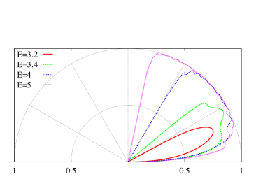
Figure 5: (Color online) Angular dependence of the transmission probability, for different values of $E$, fixing $d_{B}=1$, $d_{0}=10$, and $N=6$.

Figure 6: The conductance as a function of the energy for $N=6$ barriers with $d_{B}=1$ and $d_{0}=10$ (solid line). The dashed line is the curve given by the classical limit Eq. (16).

More remarkably we find that, rarefying the magnetic field by adding more barriers without changing the total flux $\Phi$, the transmission probability approaches the classical limit, where it is zero or one, depending on whether the incidence angle exceeds or not the angular threshold, see Fig. 3. Correspondingly, the conductance as a function of $N$ approaches the classical limit, Eq. (16), see Fig. 4. As expected, the same limit is also approached upon increasing the energy, especially for large $N$. This is clearly illustrated in Fig. 5 for the transmission, and in Fig. 6 for the conductance: one sees that already for $6$ barriers the classical limit provides a very good approximation. The classical limit is instead hardly achieved changing $d_{B}$, except when $d_{B}$ is close to the extreme values $0$ and $E/N$, see Figs. 7 and 8.

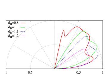
Figure 7: (Color online) Angular dependence of the transmission probability, for different values of $d_{B}$, fixing $E=2$, $d_{0}=10$, and $N=3$.

Figure 8: The conductance as a function of $d_{B}$ for $N=3$ barriers with $E=2$ and $d_{0}=10$ (solid line). The dashed line is the curve given by the classical limit Eq. (16).

In conclusion the main result of this Section is that, at fixed flux $\Phi$, the larger is the number of barriers, the more transparent is the magnetic structure. This is a purely quantum mechanical effect, peculiar to magnetic barriers.

Qualitatively this behavior can be explained as follows. To calculate the probability for a relativistic particle to go through a very thin single barrier, we can simulate the profile of $A$ with a step function with height $\Phi/N$ in order to have the same flux of a magnetic barrier with width $d_{B}=\Phi/N$. In this case the transfer matrix is simply

$${\hat{T}}={\cal W}_{0}(0^{-})^{-1}{\cal W}_{0}(0^{+}),$$ (27)

where ${\cal W}_{0}(0^{-})$ is given by Eq. (23) with $A=0$ and $k_{x}=k_{x}^{i}$, while in ${\cal W}_{0}(0^{+})$ we have $A=\Phi/N$ and consequently $k_{x}=k_{x}^{f}$. From Eq. (10) we get the following transmission probability for a single barrier

$${\cal T}_{1}(\phi)\simeq\frac{4\cos\phi\,\cos\phi_{f}\,\theta(1-|\sin\phi+\Phi/NE|)}{(\cos\phi+\cos\phi_{f})^{2}+[\Phi/(NE)]^{2}},$$ (28)

where $\phi_{f}$ is defined by $E\sin\phi_{f}=E\sin\phi+\Phi/N$. For $N$ barriers we can roughly estimate the probability for the particle to cross the magnetic structure to be

$${\cal T}_{N}(\phi)\sim{\cal T}_{1}(\phi)^{N}\,\theta(1-|\sin\phi+\Phi/E|),$$ (29)

where we have put by hand the global constraint of momentum conservation. Using the expression above we can then calculate the conductance applying Eq. (11). To simplify the calculation, in order to have a qualitative description of the conductance behavior, we further approximate $\cos\phi_{f}\simeq\cos\phi$ in Eq. (28), valid for small $\Phi/N$, and replace $\cos\phi^{2}$ with its average $1/2$, getting at the end an approximated expression for $G$ which reads

$$G\simeq G_{s}\left(\frac{2N^{2}E^{2}}{2N^{2}E^{2}+\Phi^{2}}\right)^{N},$$ (30)

being $\Phi$ the total flux for $N$ barriers. In Fig. 4 we compare the exact calculation with the approximate one given by Eq. (30), and find a surprisingly good agreement. The small discrepancy has various possible sources: the angular dependence of the transmission, which is averaged out in the approximate calculation; the finite width of the barriers; the finite separations among the barriers, which may let the particles bounce back and forth, in this way reducing the transmission. This latter effect, therefore, suppresses a bit the conductance predicted by Eq. (30).

IV Alternating magnetic barriers and wells

Next, we consider the magnetic profile in Eq. (4), illustrated in Fig. 2. In order to construct the transfer matrix in this case we need ${\cal W}_{B}$ and the partial transfer matrix for the regions with $B_{z}=-B$, which is given by

$${\cal W}_{-B}(x)=\left(\begin{array}[]{ll}D_{p+1}(-q)&D_{p+1}(q)\\ \frac{-i\sqrt{2}}{E}(p+1)D_{p}(-q)&\frac{i\sqrt{2}}{E}(p+1)D_{p}(q)\end{array}\right).$$ (31)

After some algebra, we then get

$$\hat{T} = {\cal W}_{0}^{-1}(x_{0})\,{\cal W}_{-B}(x_{0})\,\hat{T}_{0}\,\hat{T}_{1}\cdots$$ (32)

$$\quad\cdots\hat{T}_{N-2}\,\hat{T}_{N-1}\,{\cal W}_{-B}^{-1}(x_{N})\,{\cal W}_{0}(x_{N}),$$

where

$$\hat{T}_{n}={\cal W}_{-B}^{-1}(x_{n})\,{\cal W}_{B}(x_{n})\,{\cal W}_{B}^{-1}(x_{n}+d_{B})\,{\cal W}_{-B}(x_{n}+d_{B}),$$ (33)

is the transfer matrixtransfer across the $(n+1)^{\text{th}}$ magnetic barrier, and $x_{n}=n(d_{B}+d_{-B})$. Note that Eq. (33) differs from Eq. (26), since now on the right and on the left of a magnetic barrier there is a magnetic well rather than a nonmagnetic region.

As in the previous section, the numerical evaluation of $\hat{T}$ is straightforward, and the results for the transmission probability and for the conductance are illustrated in Figs. 9 to 15.

Fig. 9 shows the angular dependence of ${\cal T}$ for a single block consisting of a barrier followed by a well of different width. The plot emphasizes the very strong wave-vector dependence of the transmission, and shows that by tuning $d_{B}$ and $d_{-B}$ one can achieve very narrow transmitted beams. This suggests an interesting application of this structure as a magnetic filter, where only quasiparticles incident with an angle within a very small range are transmitted.

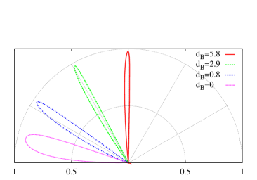
Figure 9: (Color online) Angular dependence of the transmission probability at $E=6$ through a structure consisting of one magnetic barrier of width $d_{B}$ and one magnetic well of width $d_{-B}$. We fix $d_{-B}=11.7\approx 2E$ and vary $d_{B}$ from $0$ to $5.8\approx E$.

More explicitly, in order to select a narrow beam at an angle $0<\phi<\frac{\pi}{2}$ (at fixed energy), one can choose the widths such that

$$\frac{d_{B}}{E} = (1-\sin\phi)-\varepsilon_{1},$$ (34)

$$\frac{d_{-B}}{E} = 2-\varepsilon_{2},$$ (35)

with $\varepsilon_{1,2}\ll 1$. With this choice, $\phi$ is very close to the angular threshold for the first barrier, and the well is close to be totally reflecting. The combination of these two effects leads to the narrow beam. For $-\frac{\pi}{2}<\phi<0$ it is enough to flip the magnetic field. These relations hold better at small values of $|\phi|$.

In the rest of this section, we focus on structures with $d_{B}=d_{-B}$, i.e. when the total magnetic flux through the structure vanishes.

For several blocks of barriers and wells we observe an interesting recursive effect shown in Fig. 10. There are angles at which, upon increasing $N$, the transmission takes at most $N_{m}$ values, where $N_{m}$ is the smallest number of blocks for which the transmission is perfect (i.e. ${\cal T}=1$). Some of these angles are emphasized in Fig. 10 by dashed lines. At those angles, for instance, magnetic structures with $N$ equal to integer multiples of $2$, $3$ and $5$ exhibit perfect transmission, even for small energy.

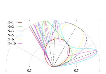
Figure 10: (Color online) Angular dependence of the transmission probability at $E=1$ and $d_{B}=d_{-B}=1$ for several values of $N$. The black dashed lines correspond to the angles for recursive transmission of multiplicity $2$ (at $\phi\approx\pi/18$), $3$ (at $\phi=-\pi/6$) and $5$ (at $\phi\approx-\pi/54$ and $\phi\approx-7\pi/18$).

Figure 11: The conductance $G/G_{0}$ at $E=1$ varying $N$ with $d_{B}=d_{-B}=1$. In the inset $d_{B}=d_{-B}=0.8$ in the same range of $N$.

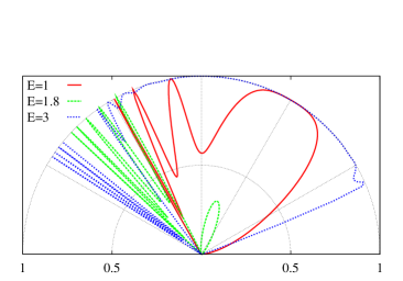
Figure 12: (Color online) Angular dependence of the transmission probability for several values of the energy $E$, for $d_{B}=d_{-B}=1$ and $N=6$.

Figure 13: The conductance $G/G_{0}$ as a function of the energy $E$ for $N=6$ with $d_{B}=d_{-B}=1$ (solid line). The dashed line is the classical limit, i.e. $(2-d_{B}/E)\,\theta(2E-d_{B})$.

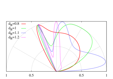
Figure 14: (Color online) Angular dependence of the transmission probability for several values of $d_{B}=d_{-B}$ with $N=3$ and $E=1$

Figure 15: The conductance $G/G_{0}$ as a function of $d_{B}=d_{-B}$ for $N=3$ with $E=1$. The dashed line is the classical limit.

These effect can be understood as follows. Suppose that, at a given angle, the transmission probability through $N_{m}$ cells has a resonance and reach the value 1. Then, for any sequence consisting of a number of cells equal to an integer multiple of $N_{m}$, the transmission is 1 again. (It is crucial here that, since the magnetic flux through each block is zero, the emergence angle always coincides with the incidence angle.) At such an angle, then, $\cal T$ can only take, upon changing $N$, at most $N_{m}$ values. Notice that perfect transmission occurs also for low energy of the incident particle, and the angular spreading of perfect transmission is also reduced by adding multiple blocks.

This effect in the transmission also reflects in the conductance. Fig. 11 shows that, for a particular set of parameters, $G$ oscillates as a function of $N$ with period $3$. However, for a different value of $d_{B}$, shown in the inset, the period is $2$. This unexpectedly strong dependence of the conductance on adding or removing blocks of barriers and wells could be exploited to design a magnetic switch for charge carriers in graphene. Moreover, we observe that the angular dependence of the transmission is abruptly modified also by changing the energy $E$ of the incident particles, see Fig. 12, or the width of the barriers $d_{B}$, Fig. 14, where we observe pronounced resonance effects. As a consequence the conductance exhibits a modulated profile as a function of both the energy and the barrier’s width, as illustrated respectively in Fig. 13 and 15.

V Periodic magnetic superlattice

We now focus on the case of a periodic magnetic superlattice. We observe that, if $d_{B}=d_{-B}$, the profile (4) can be extended to a periodic profile, illustrated in Fig. 16, where the elementary unit is given by the block formed by a barrier and a well. Imposing periodic boundary conditions on the wavefunction after a length $L=x_{N}=N\ell$ (where $\ell=2d_{B}$), i.e. $\psi(x_{0})=\psi(x_{N})$,

Figure 16: Periodic superlattice of alternating magnetic barriers and wells with $d_{B}=d_{-B}$.

and defining the matrix

$$\Omega={\cal W}_{B}^{-1}(0){\cal W}_{-B}(0){\cal W}_{-B}^{-1}(d_{B}){\cal W}_{B}(d_{B}),$$ (36)

standard calculationsmckellar lead to the quantization condition for the energy:

$$2\cos(K_{x}\ell)={\text{Tr}}\,\Omega.$$ (37)

At fixed $k_{y}$, Eq. (37) gives the energy as function of the Bloch momentum $K_{x}=\frac{2\pi n}{L}$. Notice that $K_{x}$ is related to the periodicity of the structure, and parametrizes the spectrum. It should not be confused with the $x$-component of the momentum $k_{x}$ used in the previous sections. Fig. 17 illustrates the first two bands as a function of $K_{x}$ for two values of $k_{y}$. Fig. 18 shows the contour plot for ${\text{Tr}}\,\Omega$ as function of $E$ and $k_{y}$. We find two interesting main features. First, around zero-energy there is a gap, whose width decreases for larger values of $|k_{y}|$. This is in agreement with the fact that for a magnetic profile with zero total flux there exist no zero-energy states.

Second, for some values of $k_{y}$, the group velocity $v_{y}=\frac{\partial E}{\partial k_{y}}$ diverges (see Fig. 18 close to $|k_{y}|>|E|\approx 0.3$ ). The property of superluminal velocity has already been observed for massless Klein-Gordon bosons in a periodic scalar potentialbarbier . However, to our knowledge, this is the first example in which such property is observed for massless Dirac-Weyl fermions in a periodic vector potential.

Figure 17: The spectrum for the periodic superlattice in Fig. 16 with $d_{B}=d_{-B}=1$ at $k_{y}=0$ (full points) and $k_{y}=1$ (cross poins). $K_{x}$ is the Bloch momentum.

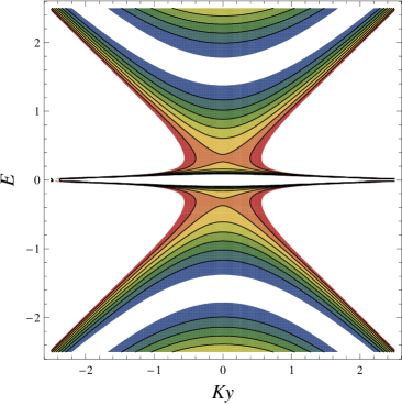
Figure 18: (Color online) The allowed spectrum, $|{\text{Tr}}\,\Omega|\leq 2$, varying $E$ and $k_{y}$, at $d_{B}=d_{-B}=1$. The contour lines correspond to the values of ${\text{Tr}}\,\Omega$ in the interval $[-2,2]$ at steps of $0.5$, increasing from blue (inner dark gray) to red (outer dark gray).

VI Summary and conclusions

In this paper we have studied the transmission of charge carriers in graphene through complex magnetic structures consisting of several magnetic barriers and wells, and the related transport properties.

We focussed on two different types of magnetic profiles. In the case of a sequence of magnetic barriers, we have found that the transparency of the structure is enhanced when the same total magnetic flux is distributed over an increasing number $N$ of barriers. The transmission probability and the conductance then approach the classical limit for large $N$, see in particular Figs. 3 and 4.

The behavior of alternating barriers and wells turns out to be even more interesting. We have shown that a single unit consisting of a barrier and a well of suitable widths can be used as a very efficient wave-vector filter for Dirac-Weyl quasiparticles, see Fig. 9. With several blocks we have observed strong resonant effects, such that at given angles one gets narrow beams perfectly transmitted even for low energy of the incident quasiparticles, see Fig. 10. As a result, the conductance is drastically modified by adding or removing blocks, see Fig. 4. This suggests possible applications as magnetic switches for charge carriers in graphene.

We hope that our paper will further stimulate experimental work on the rich physics of magnetic structures in graphene.

- (1) For recent reviews, see A.K. Geim and K.S. Novoselov, Nature Materials 6, 183 (2007); A.H. Castro Neto, F. Guinea, N.M.R. Peres, K.S. Novoselov, and A.K. Geim, cond-mat:0709.1163, to appear in Rev. Mod. Phys.
- (2) A. De Martino, L. Dell’Anna, and R. Egger, Phy. Rev. Lett. 98, 066802 (2007); Sol. State Comm. 144, 547 (2007).
- (3) S. Park and H.S. Sim, Phys. Rev. B 77, 075433 (2008).
- (4) P. Rakyta, L. Oroszlany, A. Kormanyos, C.J. Lambert, and J. Cserti, Phys. Rev. 77, 081403(R) (2008).
- (5) T.K. Ghosh, A. De Martino, W. Häusler, L. Dell’Anna, and R. Egger, Phys. Rev. B 77, 081404(R) (2008).
- (6) F. Zhai and K. Chang, Phys. Rev. B 77, 113409 (2008).
- (7) M. Tahir and K. Sabeeh, Phys. Rev. B 77, 195421 (2008).
- (8) M. Ramezani Masir, P. Vasilopoulos, A. Matulis, and F.M. Peeters, Phys. Rev. B 77, 235443 (2008).
- (9) Hengyi Xu, T. Heinzel, M. Evaldsson, and I.V. Zozoulenko, Phys. Rev. B 77, 245401 (2008)
- (10) A. Kormányos, P. Rakyta, L. Oroszlány, and J. Cserti, Phys. Rev. B 78, 045430 (2008)
- (11) S. Ghosh and M. Sarma, arXiv:0806.2951.
- (12) M.I. Katsnelson, K.S. Novoselov, and A.K. Geim, Nature Physics 2, 620 (2006); V.V. Cheianov and V.I Fal’ko, Phys. Rev. B 74, 041403(R) (2006).
- (13) K.S. Novoselov et al., Nature 438, 197 (2005); Y. Zhang et al., Nature 438, 201 (2005).
- (14) V. P. Gusynin and S.G. Sharapov, Phys. Rev. Lett. 95, 146801 (2005).
- (15) See for example M. Cerchez, S. Hugger, T. Heinzel, and N. Schulz, Phys. Rev. B 75, 035341 (2007) for a recent work, and references therein.
- (16) M.L. Leadbeater, C.L. Foden, J.H. Burroughes, M. Pepper, T.M. Burke, L.L. Wang, M.P.Grimshaw, and D.A. Ritchie, Phys. Rev. B 52, R8629 (1995).
- (17) S.J. Bending, K. von Klitzing, and K. Ploog, Phys. Rev. Lett. 65, 1060 (1990).
- (18) M. Johnson, B.R. Bennett, M.J. Yang, M.M. Miller, and B.V. Shanabrook, Appl. Phys. Lett. 71, 974 (1997); V. Kubrack et al., J. Appl. Phys. 87, 5986 (2000).
- (19) H.A. Carmona et al., Phys. Rev. Lett. 74, 3009 (1995); P.D. Ye et al., ibid. 74, 3013 (1995).
- (20) A. Nogaret, S.J. Bending, and M. Henini, Phys. Rev. Lett. 84, 2231 (2000).
- (21) K.S. Novoselov, A.K. Geim, S.V. Dubonos, Y.G. Cornelissens, F.M. Peeters, and J.C. Maan, Phys. Rev. B 65, 233312 (2002).
- (22) B. Huard, J.A. Sulpizio, N. Stander, K. Todd, B. Yang, and D. Goldhaber-Gordon, Phys. Rev. Lett. 98, 236803 (2007).
- (23) J.R. Williams, L. Di Carlo, and C.M. Marcus, Science 317, 638 (2007).
- (24) F.M. Peeters and A. Matulis, Phys. Rev. B 48, 15166 (1993); J. Reijniers, F.M. Peeters and A. Matulis, Phys. Rev. B 59, 2817 (1999). For a recent review, see also S.J. Lee, S. Souma, G. Ihm, and K.J. Chang, Physics Reports 394, 1 (2004) and refereces therein.
- (25) In all cases discussed in this paper, the transmission probability is the same at the two valleys.
- (26) From now on the magnetic flux always refers to the unit length in the -direction.
- (27) A. Matulis, F.M. Peeters, and P. Vasilopoulos, Phys. Rev. Lett. 72, 1518 (1994).
- (28) B.H.J. McKellar, G.J. Stephenson, Jr., Phys. Rev. C 35, 2262 (1987).
- (29) M. Barbier, F. M. Peeters, P. Vasilopoulos, and J. M. Pereira, Phys. Rev. B 77, 115446 (2008).
- (30) Note that, according to the usual definition, our is actually the inverse of the transfer matrix.
- (31) I.S. Ibrahim and F. M. Peeters, Phys. Rev. B 52, 17321 (1995).
- (32) I.S. Gradshteyn and I.M. Ryzhik, Table of Integrals, Series, and Products (Academic Press, Inc., New York, 1980).