#2

Dissertation
for the degree of
Doctor of Philosophy
in
Physics

Traffic Dynamics of
Computer Networks

Attila Fekete

Supervisor: Prof. Gábor Vattay, D.Sc.

Eötvös Loránd University, Faculty of Science
Graduate School in Physics
Head: Prof. Zalán Horváth, MHAS

Statistical Physics, Biological Physics and
Physics of Quantum Systems Program
Head: Prof. Jenő Kürti, D.Sc.

Department of Physics of Complex Systems
Eötvös Loránd University
Budapest, 2008

For little Bori

Chapter 1 Introduction

The objects, laws, and phenomena of Nature have been the subject of physics for hundreds of years [1]. In the second half of the 20th century, however, new interdisciplinary and applied branches of physics were developed that merged a wide range of scientific disciplines with physics including economy, biology, chemistry and geology. Most of the new branches of physics could not have evolved as they did without a specific new technological invention, namely computer technology, which developed independent from and parallel to physics. With the help of computers new research methods became available, e.g., time-series analysis, computer simulation, and data mining.

As the use of computers was spreading across the globe, computers themselves not only became increasingly useful tools for the research community, but their evolving network attracted growing academic interest. As a research tool the computer become the subject of research itself. In a pioneering work by Csabai in 1994 [2] the traffic fluctuations of the then Internet as it existed at the time was investigated. The author found that the power spectrum of the traffic delays is $1/f$-like, similarly to other collective phenomena, e.g., highway traffic. Nowadays, a new interdisciplinary science is forming to explore and model complex networks [3], in particular the Internet.

The Internet is an exceptional example of complex networks in a number of aspects. Firstly, the structure of complex networks is often the subject of research. The Internet’s infrastructure makes it possible to carry out measurements on the network cheaply and easily on an incomparable scale. Secondly, data traffic runs in the network, which adds another level of complexity to the system. Thirdly, the Internet is a human engineered physical network, which matches the complexity of some biological systems.

A useful mathematical abstraction of a network is a graph, because the number of elements of real networks is finite. However, the number of elements of complex networks is too large for the individual consideration of each network element. Moreover, the exact principles governing connections between different network components are usually unknown. Therefore, one should rely on statistical methods, specifically the tools of statistical physics, in order to describe the structure of complex networks.

The optimization of traffic performance has great practical importance. The data flows can be regarded as interacting dynamical systems superposed onto the network infrastructure. The theory of dynamical systems can therefore prove to be a useful tool for studying network traffic.

All in all the Internet is an interesting new area of academic research and several well established tools of physics can be quite useful for studying it. Since the Internet has many layers, a number of different components and, moreover, it is in constant development, it would be an impossible task to cover all aspects of its operation. Instead, I will concentrate on the dynamical modeling of the Transmission Control Protocol (TCP), the most important traffic regulatory algorithm of the current Internet. After the introductory chapter where the most important concepts of the Internet are introduced I begin my survey with the investigation of TCP operating on an elementary network configuration: a single buffer serving a link. This scenario comprises the building blocks of Internet traffic. I proceed further with the refinement of the first model, and I consider the finite storage capacity of routers in the next chapter. After the analytic and simulation study of the previous elementary single buffer models a more complex model of the Internet follows. Specifically, in the last chapter I examine the problem of efficient capacity distribution in a growing tree-like network.

1.1 The Internet

1.1.1 The short history of the Internet

The price and sheer size of the first computers restricted their applicability in the military and academic sphere. Motivated by the military needs of the United States in the cold war era a novel concept, the theory of packet-switching, was proposed by the Advanced Research Projects Agency (ARPA) to connect distant computers in a decentralized manner. The concept of packet-switching means that, contrary to connection-based circuit-switching, resources are not reserved for communication between host and destination, but data is split into small datagrams which are transmitted through the network individually. The first physical network was constructed in 1969 between four US Universities: the University of California Los Angeles, Stanford Research Institute, University of Utah and University of California Santa Barbara. This small network, called ArpaNet, is commonly perceived as the origin of the current Internet. Over the course of the following years the network grew gradually and connected more and more universities. By 1981 the number of hosts had grown to more than 200.

Based on ARPA’s research, and that of its successor DARPA the International Telecommunication Union (ITU) started developing the packet-switched network standards. In 1976 the ITU standard was approved as X.25, and provided the basis of the international and public penetration of packet switched network technology. Using the X.25 and related standards, a number of industrial companies created their own networks. The most notable was the first international packet-switched network, referred to as the International Packet Switched Service (IPSS). In 1978 IPSS was launched in Europe and the US with the collaboration of the British Post Office, Western Union International and Tymnet. By 1981 it covered Europe, North America, Australia and Hong Kong. The X.25 standard also allowed the commercial use of the network, as opposed to ArpaNet, which being a government founded project restricted its use to military and academic purposes.

In the first packet switched networks the network infrastructure itself assured reliable packet transfer between hosts. This approach made it impossible to connect different networks with different network protocols. In order to overcome this difficulty a novel concept of internetwork protocol, the TCP, was developed. With TCP the differences between different network protocols were hidden and the hosts became responsible for the reliability of the data transfer. The first specifications of TCP were given in 1974. After several years of development and testing the TCP standards were published in 1981. This paved the way for the current Internet. Since then every subnet of the Internet has adopted TCP. A detailed introduction to the protocol will be presented in the next section.

The pure network infrastructure would have been useless without user applications. The basis of many early Internet applications was Unix to Unix Copy (UUCP), developed in 1979. The most notable services using UUCP were electronic mail, Bulletin Board Systems (BBS) and Usenet News. At the dawn of the Internet era the most important service was, without doubt, email. Most of the early Internet traffic was generated by emails, but even in recent years email constitutes a significant share of Internet traffic. BBS and Usenet services were popular among home users with slow modem connections who did not have direct Internet connections. Messages, news, articles, programs or data could be uploaded and/or downloaded after the user dialed into a server. BBS and Usenet servers then periodically exchanged data via UUCP.

By the beginning of the 1990’s BBSs and Usenet had declined in importance, mainly due to the new information medium, the World Wide Web (WWW). The WWW was born of the merging of the Internet and the paradigm of hypertext in the European particle physics laboratory, the CERN. The WWW started conquering the Internet after the debut of the Mosaic web browser in 1993.

The Mosaic browser was such an enormous success that it even affected the development of the Internet itself. The Internet crossed the borders of the academic and industrial research domain and opened up to the wider public. The process was accelerated by rapid technological advances in computer technology that made personal computers a part of people’s everyday lives. The combined effect of the above led to the Internet boom in the 1990’s, when a whole new industry formed around the Internet.

By now the Internet has expanded even further than computers. Internet telephony (Voice over IP), mobile Internet (GPRS, UMTS), web cameras, wireless networks, personal digital assistants (PDAs), and sensor networks are a few examples of the current trends. The new technologies make both the structure and the traffic of the Internet more and more complex. I review these issues in the following.

1.1.2 The structure of the Internet

Since the development of the Internet was not regularized by any central authority and it has been influenced by a number of random effects the structure of the network is highly irregular. Nevertheless, the Internet can be divided into smaller segments, called Autonomous Systems (ASs). Each AS is administered by a separate organization, e.g. a university, an Internet Service Provider (ISP), or a government, and is usually organized in hierarchical, tree-like structure. ASs are connected to one another via the Internet backbone. The Internet backbone is built from high capacity links, currently up to a couple of $10\mathrm{Gbps}$. On the other end of the hierarchy end users connect to the network. The available bandwidth for end users can be in the range of $56\mathrm{Kbps}$ modems to $20\mathrm{Mbps}$ business ADSL. If we consider AS as the unit of the network, and interconnections between them as links, then we speak of AS level topology.

Internet also can be viewed on a much smaller scale consisting of two basic components: nodes and links. Nodes are devices, e.g. computers, cell phones, PDAs, routers, switches or hubs, and links are connections between them, e.g. cable (Ethernet, optical fiber), radio (WiFi, Bluetooth), infrared (IrDA), or even satellite connections. Those nodes which have multiple connections must decide in which direction they forward the through traffic. These nodes are usually referred to as routers. This detailed view is called the router level topology.

Internet topology has been studied both on AS [5, 4] and router level [6, 7, 8, 9]. On both level the Internet can be modeled as a graph from graph theory. One of the most fundamental quantities used for describing the structure of a graph is the degree sequence, which is to say the number of the neighbors of nodes. It has been found that the distribution of the degree sequence follows a power law $P(k)\sim k^{-\delta}$ on both level. The appearance of a power law indicates the scale-free nature of a particular object, so a graph the degree distribution of which follows power law is called scale-free graph. Note that in recent years the statistical properties of other scale-free networks have been investigated by the physics community as well [10, 11, 12, 13]. Examples of such networks vary from social interconnections and scientific collaborations [14] to the WWW [15].

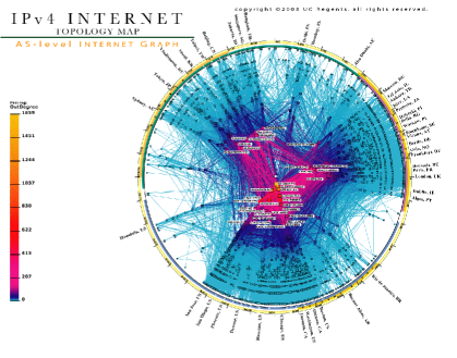
Figure 1.1: Internet AS level topology collected between 4–17 April 2005 by CAIDA [16]. The angular position of nodes corresponds to the geographical longitude of the AS headquarters. The radial position is calculated from the out-degree of ASs.

Several projects have been launched over the past decade in order to map the Internet topology. For example, the Macroscopic Topology Measurements project of CAIDA, a research group located at the University of California San Diego, surveys the Internet continuously with probe packets from a couple of dozen monitoring hosts. The visualization of the AS level map produced by CAIDA is shown in Fig. 1.1. Rocketfuel is a Internet mapping engine, developed at the University of Washington, which aims at discovering ISP router level topologies [17]. The engine makes use of routing tables to focus measurements to certain ISPs, exploits the properties of Internet Protocol (IP) routing to eliminate redundancy, and uses data from nameservers in order to classify routers.

It should be noted that the known Internet topology is only a sample of the real one. The surveyed topology is obtained from measurements, mostly via a program called traceroute. The program can discover routes between the traceroute source and given destination hosts. Since the number of sources is limited only a section of the real network can be visible in one experiment. It is therefore questionable whether the observed topology resembles the actual Internet topology. Recently it has been shown that a traceroute-based experiment can produce strong bias towards scale-free topology [18], especially when the number of sources is one or two. Moreover, it has been shown that a badly designed measurement can show scale-free topology even if the original network is regular [19].

1.1.3 Traffic on the Internet

The properties of the Internet traffic are as important as the structure of the network itself. Since the time-scale of the evolution of the network infrastructure is much larger than the time-scale of the traffic flow the network infrastructure can be considered as a static background behind the traffic dynamics. In comparison with the changes in the network traffic the dynamic changes in the network structure can be neglected.

The Internet traffic is governed by communication protocols, which can be classified into separate abstract layers according to their functionality. Each layer takes care of one or more separate tasks of data transfer and handles data towards a lower or an upper layer. User applications usually communicate with the topmost layer, whilst the lowest layer deals with the physical interaction of the hardware.

The most important classification regarding the Internet is the TCP/IP protocol suite [20, 21], which includes five or four layers. A more general and detailed model is the OSI model, which includes seven layers. The concept of layers is quite important, since it provides transparency for user applications in a very heterogeneous environment. In order to overview the mechanisms behind the Internet traffic let us introduce the four-layer model of the TCP/IP suite:

• The topmost, fourth layer of TCP/IP suite is called Application layer. It provides well-known services such as TELNET, HTTP, FTP, SSH, DNS, and SMTP. User programs should provide data to an application layer protocol in a suitable format.

• The next layer is the Transport layer, which is responsible among other things for flow control, error detection, re-transmission, and connection handling. The two most important protocols in this layer are TCP and User Datagram Protocol (UDP), which will be discussed in more detail in Section 1.2. They represent two conceptually quite different transport mechanisms: TCP provides reliable, connection-based data transfer, while UDP serves as an unreliable, connectionless, best effort transport mechanism. Other protocols at this layer are SCTP developed for Internet telephony, and RTP designed for real-time video and audio streaming.

• The following layer is referred to as the Internet layer. This layer solves the problem of addressing and routing of packets. The IP and the obsolete x.25 protocols reside in this layer. IP hides the details of the network infrastructure, and allows the interconnection of different network architectures.

• Finally, the lowest layer of the TCP/IP suite is the Network access layer, which handles physical hardware and devices. Notable examples on this layer are the ethernet, WiFi, and modems.

In order to understand the workings of the Internet, let us take the example of a typical Internet application: let us suppose that Alice wants to download a file from Bob. Since Alice wants to get an exact copy of the file, she starts an FTP session. First, the FTP protocol builds a connection between the two computers. Then the file is split into small datagrams, which are passed on to the TCP protocol on Bob’s computer. The TCP protocol adds a header to the datagrams, including a sequence number, a timestamp, and some other information which ensures reliability. Then TCP passes the datagrams on to the IP protocol, which adds its own header. The IP header contains addressing information. The resulting IP packet is put into the outgoing queue of Bob’s computer. If the queue is empty, then the packet is sent to the Network Interface Card (NIC), otherwise it has to wait until the preceding packets have been served. The NIC card disassembles the packet into ethernet frames and puts them onto the physical cable. The frames travel to the default router in Bob’s network and the router’s NIC assembles them back into an IP packet. Based on the destination address in the IP header, the router decides in which direction the packet should be forwarded and the packet is put into the outgoing queue of the corresponding direction. The packet is then disassembled and transferred again over the next cable. The procedure is repeated until the packet arrives at its final destination. The actual method of data transfer on the Network access layer can differ from the above mentioned ethernet method. If Alice uses a dial-up connection, for instance, the last step of the packet’s path is over a telephone line via a modem. At Alice’s computer the IP protocol takes the packet and passes it on to the TCP protocol. The TCP acknowledges the packet and inserts it into the missing part of the file. Finally, when Alice’s computer has received all the pieces of the file, the FTP protocol saves the whole file to its destination on her computer.

Although both packet-switched and connection-based data transfer are present in the above example, the Internet is called a packet-switched network because the Internet layer, which is the fundamental core of the Internet, utilizes solely packet-switched technology. Other layers can be either packet or circuit-switched. Ethernet traffic is packet-switched, for example, but modem traffic is carried through circuit-switched telephone lines. Higher level protocols (e.g. FTP, TELNET, SSH) are usually connection oriented, too.

Let us study the Internet layer in more detail. First of all, packets are injected into the Internet layer randomly by higher level protocols at certain source nodes. Then packets are served sequentially and forwarded to neighboring nodes by routers or, if they have arrived to their destination, removed from the network. If a router is busy serving a packet then any incoming packet is placed into a buffer and has to wait for serving. If the queue in the buffer has reached the buffer’s maximum capacity then all incoming packets are dropped until the next packet in the queue is served and an empty space becomes available in the buffer. The event when a buffer becomes full is called congestion. The above described router policy, called drop-tail, is the most wide-spread nowadays. Other router policies are also in use. The Early Random Drop (ERD) and Random Early Detection (RED) polices, for instance, drop incoming packets randomly before the buffer becomes fully occupied in order to forecast possible congestion to upper level protocols. The difference between the two policies is that the drop probability depends on the instantaneous queue length in the former case and the average queue length in the latter. It is possible to give priority to certain packets in order to provide Quality of Service (QoS) for certain applications, but routers usually serve packets in First In, First Out (FIFO) order. The serving rate of packets depends on the actual packet size and the bandwidth of the link after the buffer. Packets obviously suffer propagation delay during their delivery, is a consequence of two factors: link and from queuing delay. The former is constant for a given route, but the later varies randomly with queue lengths along the packet’s path.

The product of the link delay and link capacity, in short the bandwidth-delay product, equals the number of packets that a link can transfer simultaneously. If this quantity is large compared to the buffer size then the constant link delay is the dominant constituent of the propagation delay. Wide Area Network (WAN) links are typical examples of this. On the other hand, if the bandwidth delay product is small compared to the buffer size then the varying buffering delay is the dominant component. Such links can be found in Local Area Network (LAN). We will see later that the two scenarios induce different TCP dynamics.

It is evident that queuing theory plays an important role in the modeling of packet-switched networks in general and the Internet in particular. However, queuing theory has been developed much earlier than the advent of packet-switching technology. The first motivation and important application of queuing theory was actually a circuit-switched network, the classical telephone system.

The properties of two quantities, namely the inter-arrival and the service times of customers, affect the behavior of queuing systems most fundamentally. Other quantities, e.g. the size of the customer population, the number of operators, the system capacity etc., also have an impact on the behavior of the system, but they do not affect the essential properties of the queuing system. Both the inter-arrival and the service time series can be modeled by discrete time stochastic processes. It is usually assumed that both the inter-arrival and the service times are independent and identically-distributed (IID) random variables. Furthermore, in the most simple case, both inter-arrival and service times are memoryless processes, that is they are exponentially distributed random variables. This model is called Poisson queue, since both the number of arrivals and the number of departures in a finite time interval follow Poisson distribution. Poisson queues have been studied extensively and they proved to be excellent models of telephone call centers and telephone exchange centers. Most of the arising questions regarding Poisson queues have been answered analytically [22].

Internet traffic has been analyzed on various layers of the above TCP/IP suite. In a pioneering work by Leland et al. [23] the authors collected and studied several hours of ethernet traffic with $20$–$100\mu s$ resolution. They found that autocorrelations in the captured traffic decayed slower than exponential, that is the system has long-range memory. This result indicated problems with Poisson queuing models for packet-switched networks, since in a Poisson queuing system autocorrelations would fall exponentially [24]. Furthermore, it has been shown that the time series of the aggregated Ethernet traffic is statistically self-similar, and has fractal properties. Paxson and Floyd [25] studied the usability of Poisson models for application layer protocols and the corresponding IP traffic. They found that, though the traffic followed a 24-hour periodic pattern, Poisson processes with fixed arrival rates are acceptable models for user initiated sessions (FTP, TELNET) for intervals of one hour or less. For machine initiated sessions (SMTP, NNTP), however, the Poisson model failed even for short time-scales. Furthermore, packet level traffic deviated considerably from Poisson arrivals as well. Similar evidence has been found in WWW traffic [26]. Furthermore, it has been shown that the distribution of the packet inter-arrival times follows power law. Feldmann et al. [27] have presented the wavelet analysis of WAN traffic samples captured around the birth of the World Wide Web between ’90 and ’97. It has been found that as WWW traffic started dominating the network traffic gradually different scaling behavior appeared in short- and long-time scales. The authors concluded that TCP dynamics might be responsible for short-time scaling and application layer traffic characteristics for long-time scaling.

All the above properties are in strong contrast with the properties of the Poisson queuing systems, e.g. telephone networks, where both the correlations and the inter-arrival time distribution decay exponentially. It implies that well developed classical models, which provide excellent descriptions of circuit-switched traffic, are essentially useless for the description of the Internet. New traffic models, which provide realistic synthetic traffic, were required. A few important traffic models of the Internet will be presented in Section 2.2.

There are several theories which explain the origins of the observed long-range dependent traffic. One explanation can be that the observed traffic is the superposition of individual effects which happen on separate network layers and on very different time-scales; from several minutes of user interaction through a couple of seconds of application response until the microsecond-scale of network protocol operation. Further assumptions are that heavy-tailed file size distribution [26, 28, 29], or heavy-tailed processor time distribution is behind the phenomena. There has also been some debate on whether the TCP protocol in itself is able to generate long-range dependent traffic [30] or not [31]. The TCP’s exponential backoff mechanism is also a possible source of heavy-tailed inter-arrival times [32].

1.2 Data transport mechanisms

The Internet is an enormous data highway between computers, where data packets play the role of vehicles and links serve as the road system. As on normal highways, congestions can form at bottlenecks if the capacity of a junction is exceeded by the traffic demand.

The dynamics of the Internet traffic is governed by protocols of the Transport layer. Protocols on this layer control directly the injection rate of IP packets into the network. Almost all the Internet traffic is governed by two protocols, namely the TCP and the UDP. Therefore, understanding the operation of these protocols is very important from the point of view of traffic modeling. For example, fundamental questions are how distant hosts utilize the network infrastructure and whether they can cause persistent traffic congestion or not.

The performance of the network can be severely degraded as a result of persistent congestion. Congestion should therefore be avoided. Just such a congestion collapse did indeed occur in 1986 in the early Internet, when the useful throughput of NFSnet backbone dropped three orders of magnitude. The cause of this collapse was the faulty design of the early TCP. Instead of decreasing the sending rate of packets after detecting congestion, the early TCP actually started retransmitting lost packets, which led to an increasing sending rate and positive feedback.

1.2.1 The User Datagram Protocol

UDP is a very simple protocol, which provides a procedure for applications to send messages to other applications with a minimum of protocol mechanism [33]. Neither delivery nor duplicate protection is guaranteed by UDP. Furthermore, no congestion control is implemented in it either. UDPrealizes an open-loop control design, that is no feedback about a possible congestion is processed.

The principal uses of UDPare the Domain Name System (DNS), streaming audio and video applications (e.g. VoIP, IPTV), file sharing applications, the Trivial File Transfer Protocol (TFTP), and on-line multiplayer games, to name a few.

Since UDPlacks any congestion avoidance and control algorithm, application level programs or network-based mechanisms are required to handle congestion. In streaming applications, for example, users are often asked for the bandwidth of their access link, and UDPpackets are sent with the corresponding fixed rate. Since UDPdoes not have any feedback mechanism congestion collapse of the network due to UDP network overload is unlikely. However, aggressive network utilization should be avoided, because it can block other protocols, mainly TCP.

1.2.2 The Transmission Control Protocol

The TCP protocol is complementary to the UDPprotocol in many sense. Contrary to UDP, TCP is connection oriented, it guarantees in-order delivery and duplicate protection, congestion control and avoidance. In addition, TCP is a closed-loop design which can process feedback from packet delivery. Accordingly, TCP is a much more complex design than UDP. In this section we present an overview of TCP.

Among the applications using TCP are the WWW, email, Telnet, File Transfer Protocol (FTP), Secure Shell (ssh), to name a few. Since these applications are responsible for most of the current Internet traffic TCP is the most dominant transport protocol at the moment. Accordingly, understanding the workings of the TCP protocol has great importance in traffic modeling.

Since TCP is connection oriented, it does not start sending data immediately, like UDP. Rather it uses a three-way handshake for connection establishment. If the connection establishment phase is successful the data transfer phase follows. Finally, when all the data has been sent, the connection is terminated in the final phase. The connection establishment and termination phases are usually short and involve only negligible amount of data compared to the data transfer phase. I will therefore focus solely on the main phase, neglecting the other two phases.

In the data transfer phase the TCP receiver acknowledges every arrived packet by an acknowledgment packet (ACK). The ACK contains the sequence number of the last data packet arrived in order. If a data packet arrives out of order, then the receiver sends a duplicate ACK, that is an ACK with the same sequence number as the previous one. Duplicate ACKs directly notify the TCP sender about an out-of-order packet.

If all the packets are lost beyond a certain sequence number, then duplicate ACK cannot notify the sender about packet losses. In order to recover from such a situation, the TCP sender manages a retransmission timer. The delay of the timer, the retransmission timeout (RTO), is updated after each arriving ACK. The TCP sender measures the round-trip time (RTT), the elapsed time between the departure of a packet and the arrival of the corresponding ACK. The updated value of the RTO is calculated from the smoothed RTT, and the RTT variation as defined in [34].

Packets are acknowledged after RTT time period from packet departure if the transmission is successful. The data transfer would be very inefficient if the TCP sender waited for the ACK of the last packet before it sent the next packet. On the other hand, sending packets all at once would cause congestion. In order to reach optimum performance without causing congestion, TCP manages two sliding windows with the associated variables. On the sender side the congestion window (cwnd) limits the allowed number of unacknowledged packets. This way a cwnd number of packets is transmitted on average during a round-trip time period. Since cwnd is used directly for congestion control it is changed dynamically.

The other variable, the receiver’s advertised window (rwnd), is managed on the receiver side. Rwnd is the size of a receiver buffer which can store out-of-order packets temporally. The value of rwnd is included in every ACK, though it usually does not change. Although the limit of the unacknowledged packets is the minimum of cwnd and rwnd, the later is usually large enough not to affect data transfer in practice. Rwnd therefore plays a much less important role than cwnd. For the sake of simplicity I will assume that rwnd equals infinity. Accordingly $\min(\textit{cwnd},\textit{rwnd})$ will be replaced with cwnd in all the equations below where applicable. Let us keep in mind, however, that this is an approximation.

Internet’s packet-switched technology implies that there are no reserved resources for TCP. This approach is also called best effort delivery. Moreover, the Internet lacks any central management authority. Accordingly, TCP does not have precise information about its fair share of the network bandwidth in the ever-changing network conditions. In the previous section we have seen that buffers are able to store excess traffic temporarily, but pockets are dropped when a buffer becomes full. Flow control, the alteration of rate at which packets are sent in order to get a fair share of the network bandwidth without causing severe congestion, is one of the most important tasks of the TCP. This goal is achieved by the continuous adjustment of the congestion window and eventually the rate at which packets are sent.

Several TCP variants have been developed in recent years in order to enhance its performance in different environments [35]. These variants differ mainly in the congestion avoidance algorithm. The core concept, however, is the same in all TCP variants and has not changed significantly since its first specification in 1974. The classical TCP variants (e.g. Tahoe, Reno) try to find the fair bandwidth share by the following method: for every successfully transmitted and lost packet they increase and decrease their sending rate, respectively. This method is based on the observation that a packet loss is most likely the result of a congestion event. Note that these TCP variants obviously cause temporary congestions in the network in the long run. More recent variants often try to detect upcoming congestions beforehand via explicit congestion notifications (ECN) from routers or by detecting increasing queuing delays from RTT fluctuations (e.g. Fast TCP).

I discuss the Reno TCP variant in more detail below, since currently this is the most widespread variant in use. Its congestion control mechanism includes the following algorithms: slow start, congestion avoidance, fast recovery, and fast retransmission [36]. In figure 1.2 the schematic development of cwnd due the above congestion control algorithms is shown. There are two slow start periods at the beginning of the plot. This is possible due to the wrong initial estimate of the slow start threshold (ssthresh). After the value of ssthresh has been set to approximately half of the maximum window the fast recovery, fast retransmission (FR/FR) algorithms are able to take care of the upcoming packet losses. Note the small steps both in the slow start and the congestion avoidance phase. The steps are due to the bursty departure of packets.

\psfrag{ 0}[c][c][0.8]{$0$}\psfrag{ 5}[c][c][0.8]{$5$}\psfrag{ 10}[c][c][0.8]{$10$}\psfrag{ 15}[c][c][0.8]{$15$}\psfrag{ 20}[c][c][0.8]{$20$}\psfrag{ 25}[c][c][0.8]{$25$}\psfrag{ 30}[c][c][0.8]{$30$}\psfrag{ 35}[c][c][0.8]{$35$}\psfrag{ 40}[c][c][0.8]{$40$}\psfrag{0}[c][c][0.8]{$0$}\psfrag{5}[c][c][0.8]{$5$}\psfrag{10}[c][c][0.8]{$10$}\psfrag{15}[c][c][0.8]{$15$}\psfrag{20}[c][c][0.8]{$20$}\psfrag{25}[c][c][0.8]{$25$}\psfrag{30}[c][c][0.8]{$30$}\psfrag{35}[c][c][0.8]{$35$}\psfrag{40}[c][c][0.8]{$40$}\psfrag{45}[c][c][0.8]{$45$}\psfrag{cwnd}[c][c][1]{\emph{cwnd}}\psfrag{rtt}[c][c][1]{RTT}\psfrag{Slow start}[r][r][0.8]{Slow start}\psfrag{RTO expire}[r][r][0.8]{RTO\ expire}\psfrag{Congestion avoidance}[r][r][0.8]{Congestion avoidance}\psfrag{max packets}[r][r][0.8]{Maximum packets}\psfrag{ssthresh}[c][c][0.8]{\emph{ssthresh}}\psfrag{Fast retransmit / Fast recovery}[r][r][0.8]{Fast retransmit / Fast recovery}\includegraphics{figs/cwnd-development.eps}

Figure 1.2: Schematic plot of the development of the congestion window. The hypothetical network can handle 20 packets simultaneously, denoted by the dotted line. Cwnd might overrun this limit, because congestion is detected only after RTT latency. Note the small plateaus both in the slow start and congestion avoidance phase, which are due to the bursty arrival of packets.

Slow start and congestion avoidance

The core of the TCP congestion control mechanism is the slow start and the congestion avoidance algorithms. A state variable, the ssthresh, is used to determine whether the slow start or the congestion avoidance algorithm is used to control data transmission. When cwnd exceeds ssthresh the slow start ends, and TCP enters congestion avoidance. Ssthresh is recalculated when congestion is detected by the following formula:

$$\textit{ssthresh}=\max(\textit{cwnd}/2,2).$$ (1.1)

The slow start algorithm is used at the beginning of data transfer to probe the network and determine the available capacity. Slow start is used after repairing losses detected by the retransmission timer as well. In slow start phase TCP begins sending at most two packets, which is a “slow start” indeed. Despite what the name might suggest, however, the growth of the packet sending rate in this phase is quite fast actually: the cwnd is increased by one for every ACK. This way the sending rate is doubled in every RTT, which means exponential growth in time.

In congestion avoidance phase cwnd is increased by one every RTT period. This implies linear growth in time, which is a much more moderate development than the exponential growth in slow start. One common approximating formula for updating cwnd after every non-duplicate ACK is:

$$\textit{cwnd}\to\textit{cwnd}+\frac{1}{\textit{cwnd}}.$$ (1.2)

This formula is not precisely linear in time, but the advantage of this formula is that no auxiliary state variable is required for its application.

Fast retransmit and fast recovery

The packet sending rate is reduced drastically at the beginning of each slow start phase. Although the slow start algorithm restores cwnd to ssthresh at an exponential rate, its application might cause unnecessary performance deterioration. In order to circumvent slow start algorithm when possible, fast retransmit and fast recovery algorithms were introduced to the Reno version of TCP in 1990 [37].

The fast retransmit algorithm uses the arrival of three duplicate ACKs as an indication that a packet has been lost. After the arrival of the third duplicate ACK the sender retransmits the missing segment without waiting for the retransmission timer to expire. TCP does not enter slow start after fast retransmission, but instead starts the fast recovery algorithm. Skipping slow start is possible because each duplicate ACK indicates that a packet has been removed from the network. Therefore, newly sent packets do not stress the network further.

After fast retransmission ssthresh is set according to Eq. (1.1). In addition, cwnd is halved,

$$\textit{cwnd}\to\frac{\textit{cwnd}}{2}$$ (1.3)

and for each duplicate ACK a new segment is sent if possible. After the first non-duplicate ACK cwnd is set to ssthresh again, and TCP returns to congestion avoidance. Note that slow start might be forced when cwnd is small and duplicate ACKs are not accessible. Furthermore, if more than one packet is lost within one RTT time period, then the FR/FR algorithms may not recover from the loss either, and TCP can enter slow start algorithm instead. However, if the packet loss rate is low and cwnd is large enough, then the slow start algorithm is used only at the beginning of the TCP session, and cwnd is governed in an additive increase, multiplicative decrease (AIMD) manner by the congestion avoidance and FR/FR algorithms, respectively.

The idea behind the AIMD rule comes from the following simple control theoretical arguments [38, 39]. In general, the control of the $\lambda$th TCP’s cwnd can be given by $w_{\lambda}(t_{i+1})=f(w_{\lambda}(t_{i}),y(t_{i}))$ where $f(w,y)$ is the control function, which depends on the feedback (e.g. an ACK) from the system $y(t_{i})\in\{-,+\}$, and the last value of the window $w_{\lambda}(t_{i})$. The feedback is binary: $+$ and $-$ indicates whether to increase or decrease traffic demand, respectively. If we restrict our study to control functions, which are linear in $w_{\lambda}(t_{i})$, then we obtain

$$w_{\lambda}(t_{i+1})=a_{y(t_{i})}+b_{y(t_{i})}w_{\lambda}(t_{i}),$$ (1.4)

where the coefficients $a_{\pm}$ and $b_{\pm}$ are constants. It is obvious that the control equation (1.4) is additive if $b_{\pm}=1$, and multiplicative if $b_{\pm}\neq 1$. The most important special cases of the possible control algorithms are collected in Table 1.1. A feasible control algorithm must satisfy two important criteria: convergence to efficiency and fairness. Efficiency in this context means maximum possible usage of the available resources and fairness means equal share of the bottleneck capacity. These criteria give constraints on the coefficients $a_{\pm}$ and $b_{\pm}$. It has been shown in [39] that the convergence to efficiency and fairness is provided by the constraints $a_{+}>0$, $b_{+}\geq 1$, and $a_{-}=0$, $0\leq b_{-}<1$. Moreover, it has been shown that the convergence is fastest, when $b_{+}=1$. Therefore, the additive increase, multiplicative decrease control, which is implemented in TCP, is the optimal control algorithm.

	$b_{+}=1$	$b_{+}>1$
	$a_{+}>0$	$a_{+}=0$
$b_{-}=1$	Additive increase	Multiplicative increase
$a_{-}<0$	Additive decrease	Additive decrease
$0<b_{-}<1$	Additive increase	Multiplicative increase
$a_{-}=0$	Multiplicative decrease	Multiplicative decrease

Table 1.1: Possible control algorithms with a linear control function.

The backoff mechanism

Normally in slow start or in congestion avoidance mode, the TCP estimates the RTT and its variance from time stamps placed in ACKs. In some cases the retransmission timer might underestimate RTT at the beginning of the data transfer, and the retransmission timer might expire before the first ACK would arrive back to the TCP sender. In order to avoid the persistent expiration of the retransmission timer the so-called Karn’s algorithm [40] is applied. According to the algorithm, if the retransmission timer expires before the first ACK would return, then the value of the RTO is doubled. If the timer expires again, then the timer is doubled repeatedly a maximum six consecutive times. Since there is a definite ambiguity in estimating RTT from a retransmitted packet the ACKs of two consecutive sent packets should arrive back successfully in order for the TCP to estimate the RTT again and go back to the slow start mode.

A similar situation might occur if the packet loss rate is high. In that case, consecutive packets can be lost and the TCP might enter the backoff state, even if RTT might actually be smaller than the retransmission timer. Since the delay between packet departure is doubled, the effective bandwidth is halved after each backoff step. TCP can reduce its packet sending rate with this method below one packet per RTT.

Chapter 2 Traffic dynamics in infinite buffer

In this chapter I study the TCP dynamics on an idealized single buffer network model where the probability that a packet is lost at the buffer is negligible compared to other sources of packet loss. The case of a semi-bottleneck buffer when the size of the buffer is limited will be discussed in Chapter 3. First, I introduce the important fluid approximation of TCP congestion window dynamics in Section 2.1. In recent years many aspects of the TCP congestion avoidance phase have been clarified. The most important results of the literature are reviewed in Section 2.2. I define the network model under study in Section 2.3. My results on the analytic study of the TCP congestion window dynamics are presented in Section 2.4. The discussion of the model is given in Section 2.5. Finally, I summarize my results in Section 2.6.

2.1 The fluid approximation

The equations of motion (1.1)–(1.3) are defined at ACK arrivals. The state variables are therefore changed in discrete steps at discrete time intervals (Fig. 1.2), often referred to as “in ACK time”. Note that ”ACK time” dynamics is an essential, inherent property of TCP, because it is defined in the TCP design and does not depend on the network environment where TCP is used.

In practice the discrete-time equations of TCP dynamics can be approximated very well by continuous-time equations. Between two consecutive packet losses the congestion window is changed according to the fluid “ACK time” equation (1.2), that is

$$\frac{dW}{dt_{\textrm{ACK}}}=\frac{1}{W}.$$ (2.1)

Since the arrival of ACK packets is not uniform in time, the ACK and real time averages of important quantities, for instance the throughput, are usually different. It would be difficult and rather impractical to transform the dynamics of the state variables from ACK to real time exactly. A usual approximation is that the arrival rate of ACKs is estimated by the number of packets in flight, that is the congestion window $W$ divided by the round trip time $R$:

$$\frac{dt_{\textrm{ACK}}}{dt}=\frac{W}{R},$$ (2.2)

From the above equations one can obtain

$$\frac{dW}{dt}=\frac{1}{R}.$$ (2.3)

which is the fluid approximation of the congestion window dynamics in real time. Although this real time approximation of TCP dynamics is often sufficient, I will point out its defects. I will also present a roundabout solution to the problems based on the fundamental “ACK time” dynamics of TCP.

\psfrag{W [pkt]}[c][c][1.2]{$W[\mathrm{pkt}]$}\psfrag{T [RTT]}[c][c][1.2]{$T[s]$}\psfrag{0}[r][r][1]{$0$}\psfrag{W}[r][r][1]{$W_{m}$}\psfrag{W/2}[r][r][1]{$\frac{W_{m}}{2}$}\psfrag{RW}[r][r][1]{$W_{m}R$}\psfrag{RW/2}[r][r][1]{$\frac{W_{m}}{2}R$}\psfrag{2RW}[r][r][1]{$2W_{m}R$}\psfrag{3RW/2}[r][r][1]{$\frac{3W_{m}}{2}R$}\includegraphics{figs/aimd_example.eps}

Figure 2.1: The TCP congestion window evolution under deterministic packet loss and constant round-trip time. The congestion window $W$ varies linearly between the maximum value $W_{m}$ and its half, $W_{m}/2$.

As a simple example of the fluid model let us calculate the average throughput, the transmitted data per unit of time, of a single TCP over a lossy link [41]. Let us suppose that the round-trip time is constant and the packet loss is deterministic. Considering these assumptions the congestion window changes at a constant rate between consecutive packet loss events as (2.3). The window is halved after each packet loss event. The window evolution shown in Fig. 2.1 is therefore a periodic sawtooth in the interval $[RW_{m}/2,RW_{m}]$ and in the range of $[W_{m}/2,W_{m}]$. The length of a cycle is $RW_{m}/2$. The number of transmitted packets in a cycle equals the integral of the congestion window for one period: $N=\frac{3}{8}W_{m}^{2}$. Since in each cycle one packet is lost, the packet loss probability can be expressed as $p=1/N$. Therefore, the average throughput $\bar{X}$ can be given by

$$\bar{X}=\frac{PN}{R\frac{W_{m}}{2}}=\frac{P/p}{R\sqrt{\frac{2}{3p}}}=\frac{P}{R}\frac{c_{0}}{\sqrt{p}}$$ (2.4)

where $P$ is the size of the data packets and $c_{0}=\sqrt{\frac{3}{2}}$ is a constant. The resulting formula, often referred to as the “inverse square-root law”, expresses the impact of a network on TCP dynamics. The formula establishes a connection between throughput, an important characteristic of TCP, and packet loss probability, an attribute of the network on which TCP operates. The formula becomes inaccurate for large $p$, because multiple packet losses, which force TCP into the neglected slow start phase, are more probable in this case. The effect of multiple losses on different TCP variants is diverse, so the validity range of the formula depends on the TCP variant under consideration.

2.2 Preliminary results of traffic modeling

2.2.1 Single session models

The simple model given above can be extended considerably in a number of aspects. In a paper by Altman et al. [42] the TCP throughput for generic stationary congestion sequence was studied. The model extends the previous deterministic loss model to arbitrarily correlated loss sequences. The model is based on the following difference equation

$$X_{n+1}=\alpha S_{n}+\beta X_{n},$$ (2.5)

where $X_{n}$ is the value of the throughput just prior to the arrival of loss signal at $T_{n}$, $S_{n}=T_{n+1}-T_{n}$ is the time interval between consecutive losses, and $\alpha$ and $\beta$ are the linear growth rate and multiplicative decrease factor, respectively. From the time average of the throughput the following loss formula was derived

$$\bar{X}=\frac{P}{R\sqrt{p}}\sqrt{\frac{1+\beta}{2\left(1-\beta\right)}+\frac{1}{2}\hat{C}(0)+\sum_{k=1}^{\infty}\beta^{k}\hat{C}(k)},$$ (2.6)

where $\hat{C}(k)=\left(\mathbb{E}\left[S_{n}S_{n+k}\right]-\mathbb{E}\left[S_{n}\right]^{2}\right)/\mathbb{E}\left[S_{n}\right]^{2}$ is the normalized autocorrelation function of the loss interval process $\left(S_{n}\right)_{n\in\mathbb{N}}$. The derived formula, applied for uncorrelated Poisson process with $C(k)=0$ and $\beta=1/2$, provides the same result as (2.4). A correlated loss interval scenario was modeled with Markovian Arrival Process and the average TCP throughput was expressed with the infinitesimal generator of the arrival process. Furthermore, the authors derived bounds for the throughput in case of limited congestion window evolution and discussed the effects of timeouts.

Padhye et al. [43] have studied the steady-state throughput of TCP Reno when packet loss is detected via both duplicate ACKs and timeouts, and the throughput is limited by the receiver’s window in more detail . The probability of timeout was estimated by the packet loss probability and the congestion window. It was shown that for small packet loss the timeout probability can be approximated by $\min(1,3/W)$ and a very comprehensive loss formula has been derived.

The performance of two classic TCP versions, namely Tahoe and Reno, has been analyzed by Lakshman and Madhow [44] when the bandwidth-delay product of the bottleneck link is large compared to the buffer size. The authors estimated the average throughput for both slow start and congestion avoidance phases with deterministic and independent random losses.

In a paper by Ott et al. [45] the stationary probability distribution of the congestion window was calculated for constant packet loss probability. The authors mapped the “ACK time” point process to a continuous “subjective time” process by the mapping $W(t)=\sqrt{p}W_{\left\lfloor\frac{t}{p}\right\rfloor}$, where both the time and the state space of the discrete process is rescaled in order to obtain a well behaved process. It was shown that for $p\to 0$ the rescaled process $W(t)$ behaves as

$$\frac{dW(t)}{dt} =\frac{\alpha}{W(t)^{m}} \text{if }t\neq\tau_{k}$$ (2.7)

$$W\left(t^{+}\right) =\beta W\left(t^{-}\right) \text{if }t=\tau_{k}$$ (2.8)

where $\tau_{k}$ are the points of a Poisson process with intensity $\lambda$, $\alpha>0$ and $0<\beta<1$ are the linear growth rate and multiplicative decrease factor, respectively, $m\geq 0$, and lastly $t^{-}$ and $t^{+}$ denote the limit to $t$ from the left and from the right, respectively. The parameter values for TCP congestion avoidance algorithm are $\beta=1/2$ and $m=1$.

The stationary complementary distribution function of the process $W(t)$ has been given in the following series expansion form:

$$\bar{F}_{W}(w)=\sum_{k=0}^{\infty}R_{k}\left(c\right)\exp\left(-\frac{\eta c^{-k}}{m+1}w^{m+1}\right),$$ (2.9)

where $\eta=\lambda/\alpha$, $c=\beta^{m+1}$ and for $|c|<1$

$$\begin{split}R_{k}(c)&=\frac{1}{L(c)}\frac{(-1)^{k}c^{-\frac{1}{2}k(k+1)}}{\left(1-c\right)\left(1-c^{2}\right)\dots\left(1-c^{k}\right)},\\ L(c)&=\prod_{k=1}^{\infty}\left(1-c^{k}\right).\end{split}$$ (2.10)

“ACK”, “subjective” and real time averages and other moments of the congestion window were calculated and an inverse square root loss formula was derived.

The model has been extended for state dependent packet loss probability in [46]. State dependent loss models the interaction of the TCP with ERD queuing policy, where the packet drop probability is a function of the instantaneous queue length. It is also applicable to RED routers, where the drop probability depends on the average queue length. An iterative solution for the probability distribution function of the congestion window was derived. The authors found good agreement between the derived distribution and computer simulations.

An in-depth analysis of RED queuing dynamics was presented in [47]. The time dependent congestion window development was modeled with the stochastic differential equation

$$dW_{i}(t)=\frac{dt}{a_{i}+q(t)/C}-\frac{W_{i}(t)}{2}dN_{i}(t),$$ (2.11)

where $a_{i}$ denote the fix propagation delay of the bottleneck link, $C$ is its capacity, $q(t)$ is the queue length at time $t$ and $N_{i}(t)$ is a Poisson process with a rate that varies in time. The above equations were transformed to a system of delayed ordinary differential equations in order to obtain the dynamics of the expectation of the congestion window. The expectation value of the queue length $\bar{q}(t)$ and the RED estimate of the average queue length $\bar{x}(t)$ were approximated by two further differential equations. As a result, the authors obtained $N+2$ coupled equations for the same number of unknown variables $\left(\bar{W}_{i}(t),\bar{q}(t),\bar{x}(t)\right)$. The equations were solved numerically and were compared to computer simulations. The authors pointed out the importance of the sampling frequency of the smoothed queue length estimate. A high frequency sampling might cause unwanted oscillations in the system, while a low frequency sampling can increase the initial overshoot of the average instantaneous queue length.

2.2.2 Multiple session models

The above papers considered only a single TCP connection. In real computer networks, however, a number of TCPs might compete for the network resources. In particular the traffic of TCP sources may flow, in a parallel fashion, through a common link. Web browsing represents a good example of parallel TCP, as up to four parallel TCP sessions are started at each page download.

A possible result of TCP interaction can be that parallel TCPs are synchronized. The underlying reason for synchronization is TCP’s delayed reaction for congestion events, which keeps drop-tail bottleneck buffers congested for about an RTT time period. This temporary congestion can induce further packet losses in competing TCPs. Based on this phenomenon Lakshman and Madhow [44] supposed that the congestion window development of parallel TCPs is synchronized in the stationary congestion avoidance regime. The authors also took into consideration that the bottleneck buffer of large bandwidth-delay product connections can be either under- or over-utilized. The congestion window development was therefore split into two phases accordingly. The authors found a fixed point solution of both the duration and the average congestion window of the two phases. Finally, the average throughput of each individual connection was estimated from the window size divided by the round-trip time.

TCP synchronization is disadvantageous, since it causes performance degradation. However, this effect appears only in drop-tail queuing systems. Active queue management, such as RED and ERD, alleviate the problem of synchronization. A paper by Altman et al. [48] compared the synchronization model to one in which only one of the parallel TCPs loses a packet at a congestion event. The probability that a specific connection is affected was proportional to the throughput of the particular flow. This drop policy models RED routers. The stationary distribution of the discretized congestion window at congestion instants was calculated. The average throughput was estimated from the calculated window distribution via a semi-Markov process. The authors compared their results with simulations of a RED buffer and found that their asynchronous model surpasses the synchronous model presented in [44].

Another typical effect in multiple TCP scenario is the bias against connections with long round-trip times [49]. This effect is the fundamental consequence of TCP dynamics, and it is not affected by the queue management policy. The phenomenon can be explained qualitatively by the following simple arguments. The growth rate of the congestion window is inversely proportional to the round-trip time $R$. The average congestion window is therefore inversely proportional to $R$ as well. Furthermore, the average throughput $\bar{X}$ can be related to the average congestion window $\bar{W}$ by Little’s law from the queuing theory: $\bar{X}=\bar{W}/R$. Therefore, the throughput is approximately proportional to $1/R^{\alpha}$, with $\alpha=2$. The exponent obtained from measurements has been shown to fall in the range $1\leq\alpha<2$ due to the queuing delay ignored in the above arguments [44].

Floyd and Jacobson [50] have shown that small changes in the round-trip time might cause large differences in the throughput of different parallel TCP flows. Specifically, packets of certain TCPs can be dropped tendentiously due to a phase-effect, causing an utterly unfair bandwidth distribution. Changing the relative phase of arriving packets at the bottleneck link by slightly modifying the round-trip time can completely rearrange the bandwidth share of different TCP connections. Random effects, such as random fluctuations in the round-trip time or RED queuing policy, also alleviate the phase-effect.

2.2.3 The Network Simulator – ns-2

New models, algorithms, and analytical calculations should be validated against experiments. Without doubt the most authentic data can be obtained from Internet measurements, but the deployment of a measurement infrastructure can be quite expensive and is still very limited. Moreover, models often use simplifications which make them difficult to compare with real Internet data. Network simulators, on the other hand, provide “laboratory” environments, where every parameter of the network and the traffic can be precisely controlled. Therefore, network simulators are important tools in the hands of researchers endeavoring to carry out well controlled experiments.

One of the most widely used network simulators in the research community is the Network Simulator—ns-2 [51]. A short overview of the simulator is given next, since several analytic and numeric results of this thesis have been validated by ns-2.

The ns-2 simulator mimics every component of a real network, e.g. links, routers, queues, protocols, applications and so on. The network traffic is simulated at packet level, which is to say the course of every packet is followed from its injection into the network until its removal from it. The packet-level simulation of network traffic makes the simulator very realistic, so fine details of the simulated network traffic can be observed. The major disadvantage of a packet-level simulation is the considerable amount of computing power that it requires.

The ns-2 simulator is event-driven, that is every component might schedule events into a virtual calendar. The simulator’s scheduler runs by selecting the next earliest event for execution. During processing of events further events can be scheduled into the calendar. This event-based mechanism can also be observed in every part of the simulator, for example in the handling of data packets in ns-2. Data packets do not actually travel between virtual nodes in the simulator, but rather are scheduled for processing at different network elements instead. For example, when a packet is put onto a link for transmission the link object in the simulator only schedules the packet for the queue of the next node on the other end of the link.

The core of the simulator has been written in C++, but it also has an OTcl scripting programming interface, the object oriented extension of Tcl. The C++ core offers fast execution of the simulator. However, average users do not need to deal with C++ code in order to run simulations under ns-2. All the network elements have been bound to objects in OTcl, so complex scenarios can be built up simply and easily by writing short OTcl scripts.

2.3 The infinite-buffer network model

A very simple model of an access router connected to a complex network consists of a buffer and a link, shown in Fig. 2.2. In this regard the link is not a real connection between routers, but rather a virtual one. The influence of the network on the traffic using the access router is modeled with a few parameters of the virtual link: a fixed propagation delay $D$, bandwidth $C$, and packet loss probability $p$. This probability represents the chance of link and hardware failures [52], incorrect handling of arriving packets by routers, losses and time variations due to wireless links in the path of the connection [44], the likelihood of congestion in the instantaneous bottleneck buffer, and the effect of RED and ERD queuing policies. In this chapter I assume that the buffer is large enough that no packet loss occurs in it.

\psfrag{TCP}[c][c]{TCP}\psfrag{TCP1}[c][c]{TCP${}_{1}$}\psfrag{TCP2}[c][c]{TCP${}_{2}$}\psfrag{TCP3}[c][c]{TCP${}_{3}$}\psfrag{TCPn}[c][c]{TCP${}_{N}$}\psfrag{Sink}[c][c]{Sink}\psfrag{Sink1}[c][c]{Sink${}_{1}$}\psfrag{Sink2}[c][c]{Sink${}_{2}$}\psfrag{Sink3}[c][c]{Sink${}_{3}$}\psfrag{Sinkn}[c][c]{Sink${}_{N}$}\psfrag{Buffer}[c][c]{Buffer}\psfrag{Link}[c][c]{Link}\psfrag{Delay d}[c][c]{Delay, $D$}\psfrag{Loss rate p}[c][c]{Loss rate, $p$}\psfrag{Bandwidth C}[c][c]{Bandwidth, $C$}\psfrag{1}[c][c]{$1$}\psfrag{2}[c][c]{$2$}\psfrag{3}[c][c]{$3$}\includegraphics{figs/topology_n_inf.eps}

Figure 2.2: Idealized network model with infinite buffer capacity. Other parts of the network are modeled with link delay $D$, bandwidth $C$, and packet loss probability $p$.

Two practically important limits in respect of the role of the access buffer are: a) LANtraffic, when the bandwidth delay product of the link is small, only a few packets can be out in the link and the buffer is never empty; and b) WANtraffic, when the bandwidth delay product of the link is large, packets are in the link and the buffer is mostly empty. From now on I will refer to systems with small and large bandwidth delay products as LAN and WAN, respectively.

As I mentioned earlier in Section 1.2.2, the Internet traffic is governed mostly by TCP. I will therefore neglect UDP traffic in my simple network model and will only study the behavior of TCP dynamics.

In realistic networks many TCP sources [53] may share the resources of the access network. The difficulty of describing the parallel TCP dynamics lies in the interaction of individual TCP flows. It is obvious that the number of packets in the network injected by one of the TCP sessions affects the networking environment of the others. In particular, it contributes to the round trip times and packet losses felt by the other TCPs. Since the congestion window controls the maximum number of unacknowledged packets, understanding its distribution is crucial to describe the interaction.

While an exact treatment of nonlinear interacting systems (such as this one) is not possible in general, very efficient methods, motivated mostly by interacting physical systems, have been developed. One of the most established methods is the mean field approximation. In this approximation each subsystem operates independently in an “averaged” (or mean) environment. The average environment is calculated from the behavior of the subsystems. Finally, a fixed point of the system has to be found where the “mean” environment and the environment averaged over the independent subsystems coincide. This way we obtain a self-consistent solution which provides an approximate but quite accurate description of each subsystem.

In the case of computer networks each TCP plays the role of a subsystem, while the environment is the round trip time. First, the congestion window distribution of a TCP is calculated by assuming a given packet loss and round trip time. Next, the mean round trip time is calculated using the window distribution. Finally, a fixed point value of the round trip time is determined.

2.4 Dynamics of a single TCP

For studying the behavior of interacting TCPs by mean field approximation one should know the behavior of a single TCP first. In this section I carry out the analysis of a single TCP with the use of the fluid approximation of TCP dynamics, presented in Section 2.1.

Recall that between two consecutive losses the congestion window is governed by the continuous time differential equation (2.3):

$$\frac{dW}{dt}=\frac{1}{R(W)},$$ (2.12)

where $W\in[0,\infty[$ is the congestion window, and $R(W)$ is the round-trip time, which might depend explicitly on the value of the congestion window.

Consider, for example, a typical LAN scenario with a single TCP where the link delay is small and packet delay is caused mostly by buffering. The congestion window counts the number of unacknowledged packets, and these packets can be found on the link and in the buffer. At each packet-shift time unit a packet is shifted from the buffer into the link. The round-trip time of a freshly sent packet will be the time it should wait for the shifting of all previously sent packets in the system, which is in turn measured by the congestion window $R(W)=WP/C$.

An idealized congestion window process is shown in Fig. 2.3(b), while a simulated congestion window sequence can be seen on Fig. 2.3(a) for comparison. Numerical simulations were executed by Network Simulator (ns-2), introduced in Sec. 2.2.3. Note the small plateaus in the simulations after each cycle of the congestion window process. These plateaus are the result of the FR/FR algorithms. First, I will ignore the effect of the FR/FR algorithms, and I will consider their influence later.

\psfrag{cwnd}[c][c][1.2]{$W(t)$}\psfrag{T}[ct][cB][1.2]{$t$}\psfrag{simulation}[rB][rb][0.8]{simulation}\psfrag{2}[r][r][1]{$2$}\psfrag{4}[r][r][1]{$4$}\psfrag{6}[r][r][1]{$6$}\psfrag{8}[r][r][1]{$8$}\psfrag{10}[r][r][1]{$10$}\psfrag{12}[r][r][1]{$12$}\psfrag{14}[r][r][1]{$14$}\psfrag{16}[r][r][1]{$16$}\psfrag{18}[r][r][1]{$18$}\psfrag{20}[r][r][1]{$20$}\psfrag{1000}[r][r][1]{$1000$}\psfrag{1050}[r][r][1]{$1050$}\psfrag{1100}[r][r][1]{$1100$}\psfrag{1150}[r][r][1]{$1150$}\psfrag{1200}[r][r][1]{$1200$}\psfrag{1250}[r][r][1]{$1250$}\psfrag{1300}[r][r][1]{$1300$}\psfrag{1350}[r][r][1]{$1350$}\psfrag{1400}[r][r][1]{$1400$}\psfrag{1450}[r][r][1]{$1450$}\psfrag{1500}[r][r][1]{$1500$}\includegraphics{figs/cwnd2.eps}

(a) ns-2 simulation of LAN

\psfrag{cwnd}[c][c][1.2]{$W(t)$}\psfrag{T}[ct][cB][1.2]{$t$}\psfrag{simulation}[rB][rb][0.8]{simulation}\psfrag{2}[r][r][1]{$2$}\psfrag{4}[r][r][1]{$4$}\psfrag{6}[r][r][1]{$6$}\psfrag{8}[r][r][1]{$8$}\psfrag{10}[r][r][1]{$10$}\psfrag{12}[r][r][1]{$12$}\psfrag{14}[r][r][1]{$14$}\psfrag{16}[r][r][1]{$16$}\psfrag{18}[r][r][1]{$18$}\psfrag{20}[r][r][1]{$20$}\psfrag{1000}[r][r][1]{$1000$}\psfrag{1050}[r][r][1]{$1050$}\psfrag{1100}[r][r][1]{$1100$}\psfrag{1150}[r][r][1]{$1150$}\psfrag{1200}[r][r][1]{$1200$}\psfrag{1250}[r][r][1]{$1250$}\psfrag{1300}[r][r][1]{$1300$}\psfrag{1350}[r][r][1]{$1350$}\psfrag{1400}[r][r][1]{$1400$}\psfrag{1450}[r][r][1]{$1450$}\psfrag{1500}[r][r][1]{$1500$}\psfrag{w(t)}[cb][ct][1.2]{$W(t)$}\psfrag{t}[c][c][1.2]{$t$}\psfrag{w0}[r][r][1]{$W_{0}$}\psfrag{w1}[r][r][1]{$W_{1}$}\psfrag{d0}[c][c][1]{$\delta_{0}$}\psfrag{d1}[c][c][1]{$\delta_{1}$}\psfrag{d2}[c][c][1]{$\delta_{2}$}\psfrag{d3}[c][c][1]{$\delta_{3}$}\psfrag{d4}[c][c][1]{$\delta_{4}$}\psfrag{t0}[c][c][1]{$\tau_{0}$}\psfrag{t1}[c][c][1]{$\tau_{1}$}\psfrag{t2}[c][c][1]{$\tau_{2}$}\psfrag{t3}[c][c][1]{$\tau_{3}$}\psfrag{t4}[c][c][1]{$\tau_{4}$}\psfrag{t5}[c][c][1]{$\tau_{5}$}\includegraphics{figs/cwnd_fig-LAN-inf-b.eps}

(b) Ideal fluid model of LAN

Figure 2.3: Comparison of ns-2 simulations with the fluid approximation of the congestion avoidance process of TCP/Reno. Note the small plateaus in the simulations due to the FR/FR algorithm after each period.

In order to include more general—even hypothetical—TCP dynamics in my model the round-trip time is written in the following form:

$$R(W)=\alpha^{-1}W^{m}$$ (2.13)

with $m\geq 0$ and $\alpha>0$. Note that this notation includes the “ACK time” dynamics of TCP as well.

The fluid equation (2.12) can be written now as $\frac{dW}{dt}=\frac{\alpha}{W^{m}}$, which can be rearranged into

$$\frac{dW^{m+1}}{dt}=\alpha\left(m+1\right).$$ (2.14)

It is obvious that between two packet loss events the solution of this differential equation is

$$W^{m+1}(t)=W^{m+1}(\tau_{i})+\alpha\left(m+1\right)\left(t-\tau_{i}\right),$$ (2.15)

where $\tau_{i}$ denote the instant of the $i$^th packet loss. At $\tau_{i}$ the transformation

$$W(\tau_{i}^{+})=\beta W(\tau_{i}^{-})$$ (2.16)

is executed, where $W(\tau_{i}^{-})$ and $W(\tau_{i}^{+})$ are the congestion windows immediately before and after the time of packet loss, and $0<\beta<1$. The actual value of $\beta$ is $1/2$ in most TCP variants.

Let $W_{i}=W(\tau_{i}^{+})$ denote the congestion window immediately after the $i$^th packet loss, $\delta_{i}=\tau_{i+1}-\tau_{i}$ the length of the time interval between two losses, and $c=\beta^{m+1}$ hereafter. Since TCP is assumed to detect packet losses instantaneously in the fluid model, $W_{i+1}^{m+1}$ can be written as

$$W_{i+1}^{m+1}=\left[\beta W(\tau_{i+1})\right]^{m+1}=cW_{i}^{m+1}+\alpha\left(m+1\right)c\,\delta_{i}.$$ (2.17)

By repeated application of (2.17) one can show that the value of the congestion window immediately after the $N$^th packet loss is

$$W^{m+1}_{N}=c^{N}W^{m+1}_{0}+\alpha\left(m+1\right)\sum_{k=0}^{N-1}c^{k+1}\delta_{N-k-1}.$$ (2.18)

For $N\rightarrow\infty$ the initial value $W_{0}$ becomes insignificant and the sequence of congestion window values after the packet losses (${W_{\textrm{a.l.}}}$) can be expressed as

$${W_{\textrm{a.l.}}}^{m+1}=\lim_{N\to\infty}W^{m+1}_{N}=\alpha\left(m+1\right)\sum_{k=0}^{\infty}c^{k+1}\delta_{k}.$$ (2.19)

Note that the indexing of the $\delta_{i}$ sequence is reversed. This was allowed since, as I will show below, every $\delta_{i}$ had the same statistical properties. The reversed indexing was necessary since the infinite sum would have been meaningless without it.

In the LAN case one packet is shifted out of the buffer in each time unit. Therefore, in the fluid approximation the times between packet losses, $\delta_{i}$, are independent exponentially distributed variables. The WAN scenario is slightly different. Since there is no queue in the buffer there are periods when no packet leaves the buffer (see the small horizontal steps in Figure 2.6(a)), packets cannot be lost in those intervals. However, I assume first that times between losses are exponentially distributed in the WAN scenario as well—

$$f_{\delta_{i}}(x)=\lambda e^{-\lambda x},$$ (2.20)

where $1/\lambda$ is the average time between losses—and I will improve the model later. For the LAN case $\lambda=pC/P$, since one packet is shifted from the buffer in $P/C$ packet-shift time. Combining (2.19) and (2.20) one can obtain the distribution of ${W_{\textrm{a.l.}}}^{m+1}$:

$$f_{{W_{\textrm{a.l.}}}^{m+1}}(w)=\int\limits_{0}^{\infty}\dotsi\int\limits_{0}^{\infty}\delta\left(w-\alpha\left(m+1\right)\sum_{k=0}^{\infty}c^{k+1}x_{k}\right)\prod_{i=0}^{\infty}f_{\delta_{i}}(x_{i})\,dx_{i},$$ (2.21)

where $\delta()$ is the delta distribution. In reality only the distribution of generic values of the congestion window can be measured. Therefore, their distribution has to be derived as well. Here I show that this can be done analytically.

In general, between losses the congestion window is the sum of two random variables $W^{m+1}={W_{\textrm{a.l.}}}^{m+1}+\alpha\left(m+1\right)\tau$, where $\tau$ is a uniformly distributed random variable in the random interval $[0,\delta_{i}]$. To obtain the probability distribution of the congestion window at an arbitrary moment we have to derive the distribution of the random variable $\tau$ as well. Its distribution can be derived as follows: $\tau$ is distributed uniformly on each interval with length $\rho$, assuming $\rho$ is given. This statement can be expressed mathematically with the conditional distribution

$$f_{\tau}(t\mid\rho=x)=\frac{1}{x}\chi_{[0,x]}(t),$$ (2.22)

where $\chi_{H}(w)$ denotes the indicator function of set $H\subset\mathbb{R}$. Furthermore, the probability of selecting a random interval is proportional to the length of the given interval and the distribution of the random variable $\delta_{i}$. The proportional factor can be deduced from the normalization condition of the probability distribution:

$$f_{\rho}(x)=\frac{xf_{\delta_{i}}(x)}{\int_{0}^{\infty}xf_{\delta_{i}}(x)\,dx}=\frac{x}{\mathbb{E}[\delta_{i}]}f_{\delta_{i}}(x)=\lambda xf_{\delta_{i}}(x)$$ (2.23)

Finally, the desired distribution follows from the total probability theorem:

$$\begin{split}f_{\tau}(t)&=\int_{0}^{\infty}f_{\tau}(t\mid\rho=x)f_{\rho}(x)\,dx\\ &=\lambda\int\limits_{0}^{\infty}\lambda e^{-\lambda x}\int\limits_{0}^{x}\delta(t-y)\,dy\,dx=\lambda\int\limits_{t}^{\infty}\lambda e^{-\lambda x}\,dx=\lambda e^{-\lambda t}\end{split}$$ (2.24)

In order to calculate the distribution function of a general value of the congestion window we apply the method of the Laplace transform. As is known, the Laplace transform of the density function of the sum of independent random variables is the product of the Laplace transform of their density functions. The Laplace transform of (2.21) with respect to ${W_{\textrm{a.l.}}}^{m+1}$ can be defined as $\hat{f}_{{W_{\textrm{a.l.}}}^{m+1}}(s)=\int_{0}^{\infty}e^{-sw}f_{{W_{\textrm{a.l.}}}^{m+1}}(w)\,dw$. This can be easily evaluated and we get

$$\begin{split}\hat{f}_{{W_{\textrm{a.l.}}}^{m+1}}(s)&=\prod_{k=0}^{\infty}\left[\lambda\int\limits_{0}^{\infty}\exp\left(-s\alpha\left(m+1\right)\beta^{m\left(k+1\right)}x_{k}-\lambda x_{k}\right)\,dx_{k}\right]\\ &=\prod_{k=1}^{\infty}\frac{\lambda}{\lambda+\alpha\left(m+1\right)c^{k}s}.\end{split}$$ (2.25)

The Laplace transform of the distribution of $\alpha\left(m+1\right)\tau$ is given by

$$\hat{f}_{\alpha\left(m+1\right)\tau}(s)=\int\limits_{0}^{\infty}\frac{\lambda}{\alpha\left(m+1\right)}e^{-\frac{\lambda}{\alpha\left(m+1\right)}t}e^{-st}\,dt=\frac{\lambda}{\lambda+\alpha\left(m+1\right)s}.$$ (2.26)

Therefore, the Laplace transform of the generic $W^{m}={W_{\textrm{a.l.}}}^{m}+\alpha\left(m+1\right)\tau$ distribution is the infinite product

$$\hat{f}_{W^{m+1}}(s)=\hat{f}_{{W_{\textrm{a.l.}}}^{m+1}}(s)\,\hat{f}_{\alpha\left(m+1\right)\tau}(s)=\prod_{k=0}^{\infty}\frac{\lambda}{\lambda+\alpha\left(m+1\right)c^{k}s}.$$ (2.27)

Furthermore, we can rewrite the Laplace transform as a sum of partial fractions

$$\hat{f}_{W^{m+1}}(s)=\frac{\lambda}{\alpha\left(m+1\right)}\sum_{k=0}^{\infty}\frac{h_{k}(c)}{\frac{\lambda c^{-k}}{\alpha\left(m+1\right)}+s},$$ (2.28)

where the coefficients $h_{k}(c)$ can be obtained from the residues of the poles of $\hat{f}_{W^{m}}(s)$:

$$h_{k}(c) =\operatorname*{Res}_{-\frac{\lambda c^{-k}}{\alpha\left(m+1\right)}}\frac{\alpha\left(m+1\right)}{\lambda}\hat{f}_{W^{m+1}}(s)$$

$$=\lim_{s\to-\frac{\lambda c^{-k}}{\alpha\left(m+1\right)}}\frac{\alpha\left(m+1\right)}{\lambda}\left(s+\frac{\lambda c^{-k}}{\alpha\left(m+1\right)}\right)\prod_{l=0}^{\infty}\frac{\lambda}{\lambda+\alpha\left(m+1\right)c^{l}s}$$

$$=\frac{1}{c^{k}}\prod_{\begin{subarray}{c}l=0\\ l\neq k\end{subarray}}^{\infty}\frac{1}{1-c^{l-k}}=\frac{1}{c^{k}L(c)}\prod_{l=1}^{k}\frac{1}{1-c^{-l}},$$ (2.29)

where

$$L(c) =\prod_{l=1}^{\infty}\left(1-c^{l}\right).$$ (2.30)

It follows evidently from this formula that the relative strength of successive terms eventually decreases exponentially fast, when $k$ is large enough:

$$\frac{h_{k+1}(c)}{h_{k}(c)}=-c^{k}\frac{1}{1-c^{k+1}}\approx-c^{k}\quad\text{for $k\gg-\frac{1}{\log c}$},$$ (2.31)

therefore, only a small number of constants should be used for numerical purposes.

We can perform a term-by-term inverse Laplace transform on (2.28). The density function of $W^{m}$ can be given by

$$f_{W^{m+1}}(w)=\frac{\lambda}{\alpha\left(m+1\right)}\sum_{k=0}^{\infty}h_{k}(c)\exp\left(-\frac{\lambda c^{-k}}{\alpha\left(m+1\right)}w\right).$$ (2.32)

The distribution of the congestion window is given by a simple variable transformation

$$f_{W}(w)=\frac{\lambda}{\alpha}w^{m}\sum_{k=0}^{\infty}h_{k}(c)\exp\left(-\frac{\lambda c^{-k}}{\alpha\left(m+1\right)}w^{m+1}\right).$$ (2.33)

Finally, the complementary cumulative distribution $\bar{F}_{W}(w)=\int_{w}^{\infty}f_{W}(w^{\prime})\,dw^{\prime}$ can be given by

$$\bar{F}_{W}(w)=\sum_{k=0}^{\infty}c^{k}h_{k}(c)\exp\left(-\frac{\lambda c^{-k}}{\alpha\left(m+1\right)}w^{m+1}\right).$$ (2.34)

Note that the above formulas do not change when $\lambda$ and $\alpha$ are varied, but the $\lambda/\alpha$ ratio is kept fixed. Furthermore, the weight of the $k$^th term in the probability distribution is $c^{k}h_{k}(c)$, so the error induced by truncating terms above a threshold index can be estimated precisely: $1-\sum_{k=0}^{K}c^{k}h_{k}(c)$.

Compare the results (2.32) – (2.34) with (2.9) – (2.10). The calculation has reproduced the results of Ott et al. [45] with a slight difference in the notation. However, I have not supposed in my derivation that $p\to 0$, as Ott et al. did. Furthermore, I have shown explicitly that $\tau$ is exponentially distributed, which is missing in the previous derivation.

The moments of $W$ can be calculated from (2.32) as

$$\begin{split}\mathbb{E}[W^{r\left(m+1\right)}]&=\int_{0}^{\infty}w^{r}f_{W^{m+1}}(w)dw=\frac{\lambda}{\alpha\left(m+1\right)}\sum_{k=0}^{\infty}h_{k}(c)\int_{0}^{\infty}w^{r}e^{-\frac{\lambda c^{-k}}{\alpha\left(m+1\right)}w}dw\\ &=\left(\frac{\alpha\left(m+1\right)}{\lambda}\right)^{r}\sum_{k=0}^{\infty}c^{\left(1+r\right)k}h_{k}(c)\int_{0}^{\infty}z^{r}e^{-z}dz\\ &=\left(\frac{\alpha\left(m+1\right)}{\lambda}\right)^{r}\Gamma\left(1+r\right)\sum_{k=0}^{\infty}c^{\left(1+r\right)k}h_{k}(c),\end{split}$$ (2.35)

where $r>0$. The variable transformation $z=\frac{\lambda c^{-k}}{\alpha\left(m+1\right)}w$ was executed in the first integral, and the integral definition of the Gamma function $\Gamma(x)=\int_{0}^{\infty}z^{x-1}e^{-z}dz$ was applied in the second equation. If $r=n$ is an integer the moments can be given in closed form. For this end let us find the series expansion of the Laplace transform of $W^{m+1}$. Observe—following Ott et al.—that the product form of the Laplace transform (2.27) satisfies the following functional equation:

$$\left(1+\frac{\alpha\left(m+1\right)}{\lambda}s\right)\hat{f}_{W^{m+1}}(s)=\hat{f}_{W^{m+1}}(cs).$$ (2.36)

Differentiate $n$ times both sides of this functional equation with respect to $s$:

$$\left(1+\frac{\alpha\left(m+1\right)}{\lambda}s\right)\hat{f}^{(n)}_{W^{m+1}}(s)+n\frac{\alpha\left(m+1\right)}{\lambda}\hat{f}^{(n-1)}_{W^{m+1}}(s)=c^{n}\hat{f}^{(n)}_{W^{m+1}}(cs).$$ (2.37)

Since the $n$^th derivative of the Laplace transform at $s=0$ is related to the moments as $\mathbb{E}[W^{n\left(m+1\right)}]=(-1)^{n}\hat{f}^{(n)}_{W^{m}}(0)$, we find the following recurrence relation:

$$\left(1-c^{n}\right)\mathbb{E}[W^{n\left(m+1\right)}]=n\frac{\alpha\left(m+1\right)}{\lambda}\mathbb{E}[W^{\left(n-1\right)\left(m+1\right)}].$$ (2.38)

This recursive equation with the initial condition $\mathbb{E}[W^{0}]=1$ immediately yields

$$\mathbb{E}[W^{n\left(m+1\right)}]=n!\left(\frac{\alpha\left(m+1\right)}{\lambda}\right)^{n}\prod_{k=1}^{n}\frac{1}{1-c^{k}}.$$ (2.39)

2.5 Discussion

2.5.1 Local Area Networks

I will now confirm the validity of the above results by numerical simulations. In this section I study the LAN scenario, that is when the bandwidth-delay product of the link is much smaller than the size of the buffer. As I have pointed out earlier the parameters of the ideal LAN scenario are $m=1$, $c=\beta^{2}=1/4$, and $\alpha^{-1}\lambda=p$. The first nine numerical values of $h_{k}(c)$ are shown in Table 2.1. It can be seen that the coefficients converge to zero so quickly that it is sufficient to keep the first five terms in practical calculations.

Table 2.1: $h_{k}\left(\beta^{m+1}\right)$ coefficients with $\beta=1/2$ and $m=1$

$h_{0}$	$1$	.$4523536$	$h_{3}$	$-3$	.$2786819\cdot 10^{-2}$	$h_{6}$	$1$	.$9643078\cdot 10^{-9}$
$h_{1}$	$-1$	.$9364715$	$h_{4}$	$5$	.$1430305\cdot 10^{-4}$	$h_{7}$	$-4$	.$7959661\cdot 10^{-13}$
$h_{2}$	$5$	.$1639241\cdot 10^{-1}$	$h_{5}$	$-2$	.$0109601\cdot 10^{-6}$	$h_{8}$	$2$	.$9272701\cdot 10^{-17}$

The mean of the congestion window can be calculated from (2.35) with the parameter $r=\frac{1}{m+1}=\frac{1}{2}$:

$$\mathbb{E}[W]=\sqrt{\frac{2}{p}}\frac{\sqrt{\pi}}{2}\sum_{k=0}^{\infty}\frac{h_{k}(1/4)}{8^{k}}\approx\frac{1.5269}{\sqrt{p}},$$ (2.40)

which gives the well known inverse square-root formula. The second moment can be obtained exactly from (2.39) with $n=1$:

$$\mathbb{E}[W^{2}]=\frac{2}{p}\frac{1}{1-1/4}=\frac{8}{3p},$$ (2.41)

therefore the standard deviation is approximately

$$\sigma[W]=\sqrt{\mathbb{E}[W^{2}]-\mathbb{E}[W]^{2}}\approx\frac{0.5790}{\sqrt{p}}.$$ (2.42)

\psfrag{E[W]}[c][c][1.2]{$\mathbb{E}[W]$}\psfrag{sigma[W]}[c][c][1.2]{$\sigma[W]$}\psfrag{W_avg}[c][c][1.2]{$\left\langle W\right\rangle$}\psfrag{W_stdev}[c][c][1.2]{$\sqrt{\left\langle W^{2}\right\rangle-\left\langle W\right\rangle^{2}}$}\includegraphics{figs/avg.eps}

(a) Average vs. mean

\psfrag{E[W]}[c][c][1.2]{$\mathbb{E}[W]$}\psfrag{sigma[W]}[c][c][1.2]{$\sigma[W]$}\psfrag{W_avg}[c][c][1.2]{$\left\langle W\right\rangle$}\psfrag{W_stdev}[c][c][1.2]{$\sqrt{\left\langle W^{2}\right\rangle-\left\langle W\right\rangle^{2}}$}\includegraphics{figs/stdev.eps}

(b) Empirical standard deviation vs. standard deviation

Figure 2.4: Empirical mean and standard deviation of the congestion window as the function of the corresponding theoretical values in the range of loss probabilities $p=0.1\%$–$5\%$.

In Figure 2.4 the empirical mean and standard deviation of the congestion window is plotted as the function of the theoretical values (2.40) and (2.42), respectively. The model predicts measurement points on the diagonals, shown with dotted lines. We can see that the empirical standard deviation agrees well with the theoretical values, but the average congestion window is systematically smaller than predicted. The linear fit $f(x)=x+b$ of the data points gives an estimate for the average shift $b=-1.4141\pm 0.0611$.

The most important source of error is that FR/FR algorithms have been neglected in my idealized model, but the simulator does use these algorithms. The small plateaus appearing in the congestion window after each cycle produce bias towards the smaller window values.

In a refined model let us consider the FR/FR algorithms as well. Denote $\tilde{W}$ the fluid approximation of the extended congestion window process, which can operate in either congestion avoidance (CA) or FR/FR mode. TCP remains in FR/FR mode until the ACK of a retransmitted packet reaches the sender, that is the round-trip time before the FR/FR mode started: $R(\beta^{-1}W)$. Furthermore, the probability that a plateau forms in the window interval $[w,w+dw]$ equals the probability that the window is reduced to the given interval after a packet loss: $f_{{W_{\textrm{a.l.}}}}(w)\,dw$. The form of the distribution $f_{{W_{\textrm{a.l.}}}}(w)$ might be derived by direct calculation, but it can also be found by a simple argument: in stationary state of TCP—since the packet loss process is memoryless—packet loss can occur at every congestion window value with the same probability, supposing that the window has reached the given value. In other words the value of the “after loss” congestion window is ${W_{\textrm{a.l.}}}=\beta{W_{\textrm{b.l.}}}=\beta W$. Accordingly, the distribution of the “after loss” window is $f_{{W_{\textrm{a.l.}}}}(w)\,dw=f_{W}(\beta^{-1}w)\,d\beta^{-1}w$. On condition that TCP is in FR/FR mode the probability distribution of the congestion window is

$$f_{\tilde{W}}(w\mid\text{TCP\ in FR/FR mode})=\frac{R(\beta^{-1}w)\beta^{-1}f_{W}(\beta^{-1}w)}{\mathbb{E}[R(W)]}$$ (2.43)

On the other hand, the window distribution in the congestion avoidance mode can clearly be given by $f_{\tilde{W}}(w\mid\text{TCP\ in CA mode})=f_{W}(w)$. Now only the probabilities of the CA and FR/FR modes are required. Since each congestion avoidance phase is followed by a FR/FR mode, probabilities of the different modes are proportional to the average length of the corresponding mode. The mean length of a congestion avoidance mode is evidently the average time between two packet losses: $\mathbb{E}[\delta_{i}]=1/\lambda$. The average length of a FR/FR period, on the other hand, is simply the average length of the plateaus: $\mathbb{E}[R(W)]$. This implies that

$$\mathbb{P}(\text{TCP\ in CA mode}) =\frac{1/\lambda}{1/\lambda+\mathbb{E}[R(W)]},\quad\text{and}$$ (2.44)

$$\mathbb{P}(\text{TCP\ in FRFR mode}) =\frac{\mathbb{E}[R(W)]}{1/\lambda+\mathbb{E}[R(W)]}.$$ (2.45)

Therefore, the probability distribution of the congestion window extended by the FR/FR algorithm is

$$f_{\tilde{W}}(w)=\frac{f_{W}(w)+\frac{\lambda}{\alpha}\beta^{-\left(m+1\right)}w^{m}f_{W}(\beta^{-1}w)}{1+\frac{\lambda}{\alpha}\mathbb{E}[W^{m}]}$$ (2.46)

where (2.13), the definition of $R(W)$ has been substituted. This formula is the main result of this section. In Figure 2.5 the histogram of the congestion window simulated with ns-2 and (2.46) are compared in the range of loss probabilities $p=0.1\%$–$5.0\%$. We can see an almost perfect match between theory and simulation. In order to illustrate the improvement of the formula (2.46) on (2.33), I plotted $f_{W}(w)$ with dotted lines for comparison. I must stress here that there are no tunable parameters in (2.46) and no parameter fit has been made.

\psfrag{ 0}[c][c][1]{$0$}\psfrag{ 5}[c][c][1]{$5$}\psfrag{ 10}[c][c][1]{$10$}\psfrag{ 15}[c][c][1]{$15$}\psfrag{ 20}[c][c][1]{$20$}\psfrag{ 25}[c][c][1]{$25$}\psfrag{ 30}[c][c][1]{$30$}\psfrag{ 35}[c][c][1]{$35$}\psfrag{ 40}[c][c][1]{$40$}\psfrag{ 50}[c][c][1]{$50$}\psfrag{ 60}[c][c][1]{$60$}\psfrag{ 80}[c][c][1]{$80$}\psfrag{ 100}[c][c][1]{$100$}\psfrag{ 120}[c][c][1]{$120$}\psfrag{ 0.005}[r][r][1]{$0.005$}\psfrag{ 0.01}[r][r][1]{$0.010$}\psfrag{ 0.015}[r][r][1]{$0.015$}\psfrag{ 0.02}[r][r][1]{$0.020$}\psfrag{ 0.025}[r][r][1]{$0.025$}\psfrag{ 0.03}[r][r][1]{$0.03$}\psfrag{ 0.04}[r][r][1]{$0.04$}\psfrag{ 0.05}[r][r][1]{$0.05$}\psfrag{ 0.06}[r][r][1]{$0.06$}\psfrag{ 0.07}[r][r][1]{$0.07$}\psfrag{ 0.08}[r][r][1]{$0.08$}\psfrag{ 0.1}[r][r][1]{$0.10$}\psfrag{ 0.12}[r][r][1]{$0.12$}\psfrag{ 0.14}[r][r][1]{$0.14$}\psfrag{ 0.16}[r][r][1]{$0.16$}\psfrag{ 0.18}[r][r][1]{$0.18$}\psfrag{f_W(w)}[c][c][1.2]{$f_{W}(w)$}\psfrag{w}[ct][cB][1.2]{$w$}\psfrag{theory}[r][r][0.8]{theory CA\&FR/FR}\psfrag{theory0}[r][r][0.8]{theory CA only}\psfrag{sim}[r][r][0.8]{simulation}\includegraphics{figs/dist-LAN-p_0.1.eps}

(a) Loss rate $p=10^{-3}$

\psfrag{ 0}[c][c][1]{$0$}\psfrag{ 5}[c][c][1]{$5$}\psfrag{ 10}[c][c][1]{$10$}\psfrag{ 15}[c][c][1]{$15$}\psfrag{ 20}[c][c][1]{$20$}\psfrag{ 25}[c][c][1]{$25$}\psfrag{ 30}[c][c][1]{$30$}\psfrag{ 35}[c][c][1]{$35$}\psfrag{ 40}[c][c][1]{$40$}\psfrag{ 50}[c][c][1]{$50$}\psfrag{ 60}[c][c][1]{$60$}\psfrag{ 80}[c][c][1]{$80$}\psfrag{ 100}[c][c][1]{$100$}\psfrag{ 120}[c][c][1]{$120$}\psfrag{ 0.005}[r][r][1]{$0.005$}\psfrag{ 0.01}[r][r][1]{$0.010$}\psfrag{ 0.015}[r][r][1]{$0.015$}\psfrag{ 0.02}[r][r][1]{$0.020$}\psfrag{ 0.025}[r][r][1]{$0.025$}\psfrag{ 0.03}[r][r][1]{$0.03$}\psfrag{ 0.04}[r][r][1]{$0.04$}\psfrag{ 0.05}[r][r][1]{$0.05$}\psfrag{ 0.06}[r][r][1]{$0.06$}\psfrag{ 0.07}[r][r][1]{$0.07$}\psfrag{ 0.08}[r][r][1]{$0.08$}\psfrag{ 0.1}[r][r][1]{$0.10$}\psfrag{ 0.12}[r][r][1]{$0.12$}\psfrag{ 0.14}[r][r][1]{$0.14$}\psfrag{ 0.16}[r][r][1]{$0.16$}\psfrag{ 0.18}[r][r][1]{$0.18$}\psfrag{f_W(w)}[c][c][1.2]{$f_{W}(w)$}\psfrag{w}[ct][cB][1.2]{$w$}\psfrag{theory}[r][r][0.8]{theory CA\&FR/FR}\psfrag{theory0}[r][r][0.8]{theory CA only}\psfrag{sim}[r][r][0.8]{simulation}\psfrag{ 0.01}[r][r][1]{$0.01$}\psfrag{ 0.02}[r][r][1]{$0.02$}\includegraphics{figs/dist-LAN-p_0.5.eps}

(b) Loss rate $p=5\cdot 10^{-3}$

\psfrag{ 0}[c][c][1]{$0$}\psfrag{ 5}[c][c][1]{$5$}\psfrag{ 10}[c][c][1]{$10$}\psfrag{ 15}[c][c][1]{$15$}\psfrag{ 20}[c][c][1]{$20$}\psfrag{ 25}[c][c][1]{$25$}\psfrag{ 30}[c][c][1]{$30$}\psfrag{ 35}[c][c][1]{$35$}\psfrag{ 40}[c][c][1]{$40$}\psfrag{ 50}[c][c][1]{$50$}\psfrag{ 60}[c][c][1]{$60$}\psfrag{ 80}[c][c][1]{$80$}\psfrag{ 100}[c][c][1]{$100$}\psfrag{ 120}[c][c][1]{$120$}\psfrag{ 0.005}[r][r][1]{$0.005$}\psfrag{ 0.01}[r][r][1]{$0.010$}\psfrag{ 0.015}[r][r][1]{$0.015$}\psfrag{ 0.02}[r][r][1]{$0.020$}\psfrag{ 0.025}[r][r][1]{$0.025$}\psfrag{ 0.03}[r][r][1]{$0.03$}\psfrag{ 0.04}[r][r][1]{$0.04$}\psfrag{ 0.05}[r][r][1]{$0.05$}\psfrag{ 0.06}[r][r][1]{$0.06$}\psfrag{ 0.07}[r][r][1]{$0.07$}\psfrag{ 0.08}[r][r][1]{$0.08$}\psfrag{ 0.1}[r][r][1]{$0.10$}\psfrag{ 0.12}[r][r][1]{$0.12$}\psfrag{ 0.14}[r][r][1]{$0.14$}\psfrag{ 0.16}[r][r][1]{$0.16$}\psfrag{ 0.18}[r][r][1]{$0.18$}\psfrag{f_W(w)}[c][c][1.2]{$f_{W}(w)$}\psfrag{w}[ct][cB][1.2]{$w$}\psfrag{theory}[r][r][0.8]{theory CA\&FR/FR}\psfrag{theory0}[r][r][0.8]{theory CA only}\psfrag{sim}[r][r][0.8]{simulation}\psfrag{ 0.01}[r][r][1]{$0.01$}\psfrag{ 0.02}[r][r][1]{$0.02$}\includegraphics{figs/dist-LAN-p_1.0.eps}

(c) Loss rate $p=0.01$

\psfrag{ 0}[c][c][1]{$0$}\psfrag{ 5}[c][c][1]{$5$}\psfrag{ 10}[c][c][1]{$10$}\psfrag{ 15}[c][c][1]{$15$}\psfrag{ 20}[c][c][1]{$20$}\psfrag{ 25}[c][c][1]{$25$}\psfrag{ 30}[c][c][1]{$30$}\psfrag{ 35}[c][c][1]{$35$}\psfrag{ 40}[c][c][1]{$40$}\psfrag{ 50}[c][c][1]{$50$}\psfrag{ 60}[c][c][1]{$60$}\psfrag{ 80}[c][c][1]{$80$}\psfrag{ 100}[c][c][1]{$100$}\psfrag{ 120}[c][c][1]{$120$}\psfrag{ 0.005}[r][r][1]{$0.005$}\psfrag{ 0.01}[r][r][1]{$0.010$}\psfrag{ 0.015}[r][r][1]{$0.015$}\psfrag{ 0.02}[r][r][1]{$0.020$}\psfrag{ 0.025}[r][r][1]{$0.025$}\psfrag{ 0.03}[r][r][1]{$0.03$}\psfrag{ 0.04}[r][r][1]{$0.04$}\psfrag{ 0.05}[r][r][1]{$0.05$}\psfrag{ 0.06}[r][r][1]{$0.06$}\psfrag{ 0.07}[r][r][1]{$0.07$}\psfrag{ 0.08}[r][r][1]{$0.08$}\psfrag{ 0.1}[r][r][1]{$0.10$}\psfrag{ 0.12}[r][r][1]{$0.12$}\psfrag{ 0.14}[r][r][1]{$0.14$}\psfrag{ 0.16}[r][r][1]{$0.16$}\psfrag{ 0.18}[r][r][1]{$0.18$}\psfrag{f_W(w)}[c][c][1.2]{$f_{W}(w)$}\psfrag{w}[ct][cB][1.2]{$w$}\psfrag{theory}[r][r][0.8]{theory CA\&FR/FR}\psfrag{theory0}[r][r][0.8]{theory CA only}\psfrag{sim}[r][r][0.8]{simulation}\psfrag{ 0.01}[r][r][1]{$0.01$}\psfrag{ 0.02}[r][r][1]{$0.02$}\includegraphics{figs/dist-LAN-p_2.0.eps}

(d) Loss rate $p=0.02$

\psfrag{ 0}[c][c][1]{$0$}\psfrag{ 5}[c][c][1]{$5$}\psfrag{ 10}[c][c][1]{$10$}\psfrag{ 15}[c][c][1]{$15$}\psfrag{ 20}[c][c][1]{$20$}\psfrag{ 25}[c][c][1]{$25$}\psfrag{ 30}[c][c][1]{$30$}\psfrag{ 35}[c][c][1]{$35$}\psfrag{ 40}[c][c][1]{$40$}\psfrag{ 50}[c][c][1]{$50$}\psfrag{ 60}[c][c][1]{$60$}\psfrag{ 80}[c][c][1]{$80$}\psfrag{ 100}[c][c][1]{$100$}\psfrag{ 120}[c][c][1]{$120$}\psfrag{ 0.005}[r][r][1]{$0.005$}\psfrag{ 0.01}[r][r][1]{$0.010$}\psfrag{ 0.015}[r][r][1]{$0.015$}\psfrag{ 0.02}[r][r][1]{$0.020$}\psfrag{ 0.025}[r][r][1]{$0.025$}\psfrag{ 0.03}[r][r][1]{$0.03$}\psfrag{ 0.04}[r][r][1]{$0.04$}\psfrag{ 0.05}[r][r][1]{$0.05$}\psfrag{ 0.06}[r][r][1]{$0.06$}\psfrag{ 0.07}[r][r][1]{$0.07$}\psfrag{ 0.08}[r][r][1]{$0.08$}\psfrag{ 0.1}[r][r][1]{$0.10$}\psfrag{ 0.12}[r][r][1]{$0.12$}\psfrag{ 0.14}[r][r][1]{$0.14$}\psfrag{ 0.16}[r][r][1]{$0.16$}\psfrag{ 0.18}[r][r][1]{$0.18$}\psfrag{f_W(w)}[c][c][1.2]{$f_{W}(w)$}\psfrag{w}[ct][cB][1.2]{$w$}\psfrag{theory}[r][r][0.8]{theory CA\&FR/FR}\psfrag{theory0}[r][r][0.8]{theory CA only}\psfrag{sim}[r][r][0.8]{simulation}\psfrag{ 0.01}[r][r][1]{$0.01$}\psfrag{ 0.02}[r][r][1]{$0.02$}\includegraphics{figs/dist-LAN-p_4.0.eps}

(e) Loss rate $p=0.04$

\psfrag{ 0}[c][c][1]{$0$}\psfrag{ 5}[c][c][1]{$5$}\psfrag{ 10}[c][c][1]{$10$}\psfrag{ 15}[c][c][1]{$15$}\psfrag{ 20}[c][c][1]{$20$}\psfrag{ 25}[c][c][1]{$25$}\psfrag{ 30}[c][c][1]{$30$}\psfrag{ 35}[c][c][1]{$35$}\psfrag{ 40}[c][c][1]{$40$}\psfrag{ 50}[c][c][1]{$50$}\psfrag{ 60}[c][c][1]{$60$}\psfrag{ 80}[c][c][1]{$80$}\psfrag{ 100}[c][c][1]{$100$}\psfrag{ 120}[c][c][1]{$120$}\psfrag{ 0.005}[r][r][1]{$0.005$}\psfrag{ 0.01}[r][r][1]{$0.010$}\psfrag{ 0.015}[r][r][1]{$0.015$}\psfrag{ 0.02}[r][r][1]{$0.020$}\psfrag{ 0.025}[r][r][1]{$0.025$}\psfrag{ 0.03}[r][r][1]{$0.03$}\psfrag{ 0.04}[r][r][1]{$0.04$}\psfrag{ 0.05}[r][r][1]{$0.05$}\psfrag{ 0.06}[r][r][1]{$0.06$}\psfrag{ 0.07}[r][r][1]{$0.07$}\psfrag{ 0.08}[r][r][1]{$0.08$}\psfrag{ 0.1}[r][r][1]{$0.10$}\psfrag{ 0.12}[r][r][1]{$0.12$}\psfrag{ 0.14}[r][r][1]{$0.14$}\psfrag{ 0.16}[r][r][1]{$0.16$}\psfrag{ 0.18}[r][r][1]{$0.18$}\psfrag{f_W(w)}[c][c][1.2]{$f_{W}(w)$}\psfrag{w}[ct][cB][1.2]{$w$}\psfrag{theory}[r][r][0.8]{theory CA\&FR/FR}\psfrag{theory0}[r][r][0.8]{theory CA only}\psfrag{sim}[r][r][0.8]{simulation}\psfrag{ 0.01}[r][r][1]{$0.01$}\psfrag{ 0.02}[r][r][1]{$0.02$}\includegraphics{figs/dist-LAN-p_5.0.eps}

(f) Loss rate $p=0.05$

Figure 2.5: Histograms and theoretical distributions of congestion windows in LAN. Network parameters are $C=256\,kb/s$, $P=1500\,\mathit{byte}$, and $D=0\,s$.

Let us calculate the moments of $\tilde{W}$:

$$\mathbb{E}[{\tilde{W}}^{k}]=\frac{\mathbb{E}[W^{k}]+\beta^{k}\frac{\lambda}{\alpha}\mathbb{E}[W^{m+k}]}{1+\frac{\lambda}{\alpha}\mathbb{E}[W^{m}]}.$$ (2.47)

As an important special case we can calculate the correction of the FR/FR algorithms to the mean of the congestion window:

$$\mathbb{E}[\tilde{W}-W]=-\frac{\lambda}{\alpha}\frac{\mathbb{E}[W]\mathbb{E}[W^{m}]-\beta\mathbb{E}[W^{m+1}]}{1+\frac{\lambda}{\alpha}\mathbb{E}[W^{m}]}$$ (2.48)

If the formula (2.35) is substituted into the above equation one can obtain the dependence of the correction on $\lambda/\alpha$. Specifically, for $m=1$: $\mathbb{E}[\tilde{W}-W]\approx-\frac{0.9981}{1+1.5269\sqrt{\frac{\lambda}{\alpha}}}$. Interestingly, the correction tends to a constant in the small loss limit: $\lim_{\lambda/\alpha\to 0}\mathbb{E}[\tilde{W}-W]\approx-0.9981$. In the range of loss probabilities $p=\lambda/\alpha=10^{-4}$–$5\cdot 10^{-2}$, investigated by simulations, the correction to the congestion window average is between $-0.8659$ and $0.9831$, which is less than observed in Fig. 2.4(a). The remaining discrepancy comes from the difference between the continuous and the fluid value of $W$. In the simulation the congestion window is not only halved its integer part is also taken. This discrepancy accounts for approximately $-0.5$ unit shift on average. The slow start mechanism, which becomes more and more dominant as the loss probability increases, also makes the small window values more probable. However, these effects are beyond the scope of the applied fluid model.

2.5.2 Wide Area Networks

I turn now to the WAN scenario, where buffering delay is very small compared to the link delay. A typical congestion window sequence is shown in Figure 2.6 with $D=1s$ and $p=0.01$.

\psfrag{ 0}[r][r][1]{$0$}\psfrag{ 4}[r][r][1]{$4$}\psfrag{ 5}[r][r][1]{$5$}\psfrag{ 6}[r][r][1]{$6$}\psfrag{ 7}[r][r][1]{$7$}\psfrag{ 8}[r][r][1]{$8$}\psfrag{ 9}[r][r][1]{$9$}\psfrag{ 10}[r][r][1]{$10$}\psfrag{ 15}[r][r][1]{$15$}\psfrag{ 20}[r][r][1]{$20$}\psfrag{ 25}[r][r][1]{$25$}\psfrag{ 200}[c][c][1]{$200$}\psfrag{ 250}[c][c][1]{$250$}\psfrag{ 300}[c][c][1]{$300$}\psfrag{ 350}[c][c][1]{$350$}\psfrag{ 374}[c][c][1]{$374$}\psfrag{ 376}[c][c][1]{$376$}\psfrag{ 378}[c][c][1]{$378$}\psfrag{ 380}[c][c][1]{$380$}\psfrag{ 382}[c][c][1]{$382$}\psfrag{ 384}[c][c][1]{$384$}\psfrag{ 400}[c][c][1]{$400$}\psfrag{ 450}[c][c][1]{$450$}\psfrag{ 500}[c][c][1]{$500$}\psfrag{simulation}[r][r][0.8]{simulation}\psfrag{cwnd}[r][r][1.2]{$W(t)$}\psfrag{T}[c][c][1.2]{$t$}\includegraphics{figs/cwnd-WAN.eps}

(a) ns-2 simulation of WAN

\psfrag{ 0}[r][r][1]{$0$}\psfrag{ 4}[r][r][1]{$4$}\psfrag{ 5}[r][r][1]{$5$}\psfrag{ 6}[r][r][1]{$6$}\psfrag{ 7}[r][r][1]{$7$}\psfrag{ 8}[r][r][1]{$8$}\psfrag{ 9}[r][r][1]{$9$}\psfrag{ 10}[r][r][1]{$10$}\psfrag{ 15}[r][r][1]{$15$}\psfrag{ 20}[r][r][1]{$20$}\psfrag{ 25}[r][r][1]{$25$}\psfrag{ 200}[c][c][1]{$200$}\psfrag{ 250}[c][c][1]{$250$}\psfrag{ 300}[c][c][1]{$300$}\psfrag{ 350}[c][c][1]{$350$}\psfrag{ 374}[c][c][1]{$374$}\psfrag{ 376}[c][c][1]{$376$}\psfrag{ 378}[c][c][1]{$378$}\psfrag{ 380}[c][c][1]{$380$}\psfrag{ 382}[c][c][1]{$382$}\psfrag{ 384}[c][c][1]{$384$}\psfrag{ 400}[c][c][1]{$400$}\psfrag{ 450}[c][c][1]{$450$}\psfrag{ 500}[c][c][1]{$500$}\psfrag{simulation}[r][r][0.8]{simulation}\psfrag{cwnd}[r][r][1.2]{$W(t)$}\psfrag{T}[c][c][1.2]{$t$}\psfrag{w0}[r][r][1]{$W_{0}$}\psfrag{w1}[r][r][1]{$W_{1}$}\psfrag{d0}[c][c][1]{$\delta_{0}$}\psfrag{d1}[c][c][1]{$\delta_{1}$}\psfrag{d2}[c][c][1]{$\delta_{2}$}\psfrag{d3}[c][c][1]{$\delta_{3}$}\psfrag{d4}[c][c][1]{$\delta_{4}$}\psfrag{t0}[c][c][1]{$\tau_{0}$}\psfrag{t1}[c][c][1]{$\tau_{1}$}\psfrag{t2}[c][c][1]{$\tau_{2}$}\psfrag{t3}[c][c][1]{$\tau_{3}$}\psfrag{t4}[c][c][1]{$\tau_{4}$}\psfrag{t5}[c][c][1]{$\tau_{5}$}\psfrag{ACTIVE}[ct][cb][1]{Active}\psfrag{IDLE}[cb][ct][1]{Idle}\psfrag{JUMP1}[cb][ct][1]{Jump}\psfrag{JUMP2}[cb][ct][1]{Jump}\psfrag{JUMP3}[cb][ct][1]{Jump}\psfrag{JUMP4}[cb][ct][1]{Jump}\includegraphics{figs/cwnd-WAN-detail.eps}

(b) Details of the cwnd in the bounded box

Figure 2.6: The congestion avoidance process of TCP in WAN setup. The global congestion window development is seemingly linear, but the detailed plot on Figure 2.6(b) shows a different picture. The globally linear growth is composed of alternating idle and LAN-like active periods. See the discussion in the text.

The applicability of the developed model depends on two crucial factors: the validity of the exponential inter-loss distribution (2.20) and the validity of (2.13), the dependence of round-trip time on the congestion window. The difficulty of the WAN scenario is that—as I mentioned earlier—there are periods when no packet leaves the buffer. This effect corrupts the validity of both assumptions. Packets cannot be lost during idle periods, so the inter-loss time distribution deviates from exponential distribution. Furthermore, if we assume that the round-trip time is constant, $R(W)=2D$, then the solution of the equation of motion (2.15) predicts linear congestion window development, which corresponds to $m=0$ in the model. However, a typical sequence of congestion windows, displayed in Fig. 2.6(b), shows step-like growth instead. Another difficulty is that even if the inter-arrival times can be approximated with an exponential distribution, the connection between the packet loss probability $p$ and the parameter of the distribution $\lambda$ is unknown.

Given these concerns I approach the congestion window development in a WAN network in a manner different from simple linear growth, the model applied exclusively in the literature. First of all let us investigate the window development in congestion avoidance mode in more detail. The fine structure of the congestion window is shown in Fig. 2.6(b). During the active period of TCP, when ACKs are arriving back to the sender (in “ACK time”), the congestion window is being increased the same way as in a LAN network. The difference from LAN in a WAN scenario is that an idle period follows with a constant congestion window. Since $W$ packets are transferred in an active period, the length of an active period is $W/\alpha$. The following idle period is $2D-W/\alpha$ long, because the total length of an active and the succeeding idle period is precisely one round-trip time, $2D$.

Let $W^{*}$ denote the congestion window idle periods included. If the plateaus corresponding to idle periods are approximated as if they were blurred evenly on the active periods, then—analogously to the FR/FR mode in LAN—the conditional distribution of the congestion window in idle mode of TCP can be formulated as

$$f_{W^{*}}(w\mid\text{TCP\ in IDLE mode})=\frac{\frac{2D-w/\alpha}{w/\alpha}f_{W}(w)\,\Theta(2D-w/\alpha)}{\mathbb{E}\left[\frac{2D-W/\alpha}{W/\alpha}\Theta(2D-W/\alpha)\right]}.$$ (2.49)

Only the probabilities of idle, CA and FR/FR modes are required. The probability of each mode is proportional to the average time TCP spends in the particular mode. Considering the idle mode, the average length of a plateau in one ACK increment is $\mathbb{E}\left[\frac{2D-W/\alpha}{W/\alpha}\Theta(2D-W/\alpha)\right]$. Moreover, the window is increased $\mathbb{E}[\delta_{i}]=1/\lambda$ times in one loss cycle on average. Accordingly, the probability of idle mode is

$$\mathbb{P}(\text{TCP\ in IDLE mode})=\frac{\mathbb{E}\left[\frac{2\alpha D-W}{W}\Theta(2\alpha D-W)\right]/\lambda}{1/\lambda+\mathbb{E}[R(W)]+\mathbb{E}\left[\frac{2\alpha D-W}{W}\Theta(2\alpha D-W)\right]/\lambda}.$$ (2.50)

The probabilities of CA and FR/FR modes in Eqs. (2.44) and (2.45) should be modified proportionately. As a result we obtain

$$f_{W^{*}}(w)=\frac{f_{W}(w)+\frac{\lambda}{\alpha}\beta^{-\left(m+1\right)}w^{m}f_{W}(\beta^{-1}w)+\frac{2\alpha D-w}{w}f_{W}(w)\,\Theta(2\alpha D-w)}{\bar{F}_{W}(2\alpha D)+\frac{\lambda}{\alpha}\mathbb{E}[W^{m}]+2\alpha D\,\mathbb{E}\left[\frac{1}{W}\Theta(2\alpha D-W)\right]}$$ (2.51)

for the congestion window distribution, where I used that $\mathbb{E}[\Theta(2\alpha D-W)]=\int_{0}^{2\alpha D}f_{W}(w)\,dw=1-\bar{F}_{W}(2\alpha D)$. The truncated expectation of $1/W$ can be obtained similarly to (2.35) with $r=-\frac{1}{m+1}$, but one should include the incomplete Gamma function $\Gamma(z,x)=\int_{x}^{\infty}x^{z-1}e^{-x}\,dx$ as well:

$$\begin{split}&\mathbb{E}\left[\frac{1}{W}\Theta(2\alpha D-W)\right]=\int_{0}^{2\alpha D}\frac{1}{w}f_{W}(w)\,dw\\ =&\mathbb{E}\left[\frac{1}{W}\right]-\left(\frac{\lambda}{\alpha\left(m+1\right)}\right)^{\frac{1}{m+1}}\sum_{k=0}^{\infty}\Gamma\left(\frac{m}{m+1},\frac{2\lambda Dc^{-k}}{m+1}\right)c^{\frac{mk}{m+1}}h_{k}(c).\end{split}$$ (2.52)

The moments of $W^{*}$ can be given easily:

$$\mathbb{E}\bigl{[}{W^{*}}^{k}\bigr{]}=\frac{\mathbb{E}[W^{k}]+\frac{\lambda}{\alpha}\beta^{k}\mathbb{E}[W^{m+k}]+\mathbb{E}\left[\left(2\alpha D\,W^{k-1}-W^{k}\right)\Theta(2\alpha D-W)\right]}{\bar{F}_{W}(2\alpha D)+\frac{\lambda}{\alpha}\mathbb{E}[W^{m}]+2\alpha D\,\mathbb{E}\left[\frac{1}{W}\Theta(2\alpha D-W)\right]}\,.$$ (2.53)

The distribution and moments of the ideal WAN scenario can be obtained from (2.51) and (2.53) in the $\alpha D\to\infty$ limit:

$$\lim_{\alpha D\to\infty}f_{W^{*}}(w) =\frac{1}{w\mathbb{E}\left[\frac{1}{W}\right]}f_{W}(w) \lim_{\alpha D\to\infty}\mathbb{E}\bigl{[}{W^{*}}^{k}\bigr{]} =\frac{\mathbb{E}[W^{k-1}]}{\mathbb{E}\left[\frac{1}{W}\right]}.$$ and (2.54)

Note that the formula (2.51) at $D=0$ reduces to (2.46), derived earlier for an ideal LAN scenario with CA and FR/FR modes. Note further that (2.51) is applicable not only for the ideal WAN or LAN scenarios, but also for for the most generic configuration. Moreover, I would like to emphasize that the parameters of the model can be obtained from the intrinsic “ACK time” dynamics of TCP, and no parameter fitting is necessary. Specifically, for TCP/Reno the parameters are $m=1$, $\lambda/\alpha=p$, $\beta=1/2$ and $2\alpha D$ is the bandwidth-delay product measured in packet units.

\psfrag{ 0}[c][c][1]{$0$}\psfrag{ 5}[c][c][1]{$5$}\psfrag{ 10}[c][c][1]{$10$}\psfrag{ 15}[c][c][1]{$15$}\psfrag{ 20}[c][c][1]{$20$}\psfrag{ 25}[c][c][1]{$25$}\psfrag{ 30}[c][c][1]{$30$}\psfrag{ 35}[c][c][1]{$35$}\psfrag{ 40}[c][c][1]{$40$}\psfrag{ 50}[c][c][1]{$50$}\psfrag{ 60}[c][c][1]{$60$}\psfrag{ 80}[c][c][1]{$80$}\psfrag{ 100}[c][c][1]{$100$}\psfrag{ 120}[c][c][1]{$120$}\psfrag{ 140}[c][c][1]{$140$}\psfrag{ 150}[c][c][1]{$150$}\psfrag{ 160}[c][c][1]{$160$}\psfrag{ 180}[c][c][1]{$180$}\psfrag{ 200}[c][c][1]{$200$}\psfrag{ 250}[c][c][1]{$250$}\psfrag{ 300}[c][c][1]{$300$}\psfrag{ 350}[c][c][1]{$350$}\psfrag{ 400}[c][c][1]{$400$}\psfrag{ 0.001}[r][r][1]{$0.001$}\psfrag{ 0.002}[r][r][1]{$0.002$}\psfrag{ 0.003}[r][r][1]{$0.003$}\psfrag{ 0.004}[r][r][1]{$0.004$}\psfrag{ 0.005}[r][r][1]{$0.005$}\psfrag{ 0.006}[r][r][1]{$0.006$}\psfrag{ 0.007}[r][r][1]{$0.007$}\psfrag{ 0.008}[r][r][1]{$0.008$}\psfrag{ 0.009}[r][r][1]{$0.009$}\psfrag{ 0.01}[r][r][1]{$0.01$}\psfrag{ 0.012}[r][r][1]{$0.012$}\psfrag{ 0.014}[r][r][1]{$0.014$}\psfrag{ 0.015}[r][r][1]{$0.015$}\psfrag{ 0.016}[r][r][1]{$0.016$}\psfrag{ 0.018}[r][r][1]{$0.018$}\psfrag{ 0.02}[r][r][1]{$0.02$}\psfrag{ 0.025}[r][r][1]{$0.025$}\psfrag{ 0.03}[r][r][1]{$0.03$}\psfrag{ 0.04}[r][r][1]{$0.04$}\psfrag{ 0.05}[r][r][1]{$0.05$}\psfrag{ 0.06}[r][r][1]{$0.06$}\psfrag{ 0.07}[r][r][1]{$0.07$}\psfrag{ 0.08}[r][r][1]{$0.08$}\psfrag{ 0.09}[r][r][1]{$0.09$}\psfrag{ 0.1}[r][r][1]{$0.1$}\psfrag{ 0.15}[r][r][1]{$0.15$}\psfrag{ 0.2}[r][r][1]{$0.2$}\psfrag{ 0.25}[r][r][1]{$0.25$}\psfrag{f_W(w)}[c][c][1.2]{$f_{W}(w)$}\psfrag{w}[ct][cB][1.2]{$w$}\psfrag{theory}[r][r][0.8]{theory}\psfrag{ack-wise}[r][r][0.8]{theory---active mode}\psfrag{sim}[r][r][0.8]{simulation}\includegraphics{figs/dist-WAN-p_0.01.eps}

(a) Loss rate $p=10^{-4}$

\psfrag{ 0}[c][c][1]{$0$}\psfrag{ 5}[c][c][1]{$5$}\psfrag{ 10}[c][c][1]{$10$}\psfrag{ 15}[c][c][1]{$15$}\psfrag{ 20}[c][c][1]{$20$}\psfrag{ 25}[c][c][1]{$25$}\psfrag{ 30}[c][c][1]{$30$}\psfrag{ 35}[c][c][1]{$35$}\psfrag{ 40}[c][c][1]{$40$}\psfrag{ 50}[c][c][1]{$50$}\psfrag{ 60}[c][c][1]{$60$}\psfrag{ 80}[c][c][1]{$80$}\psfrag{ 100}[c][c][1]{$100$}\psfrag{ 120}[c][c][1]{$120$}\psfrag{ 140}[c][c][1]{$140$}\psfrag{ 150}[c][c][1]{$150$}\psfrag{ 160}[c][c][1]{$160$}\psfrag{ 180}[c][c][1]{$180$}\psfrag{ 200}[c][c][1]{$200$}\psfrag{ 250}[c][c][1]{$250$}\psfrag{ 300}[c][c][1]{$300$}\psfrag{ 350}[c][c][1]{$350$}\psfrag{ 400}[c][c][1]{$400$}\psfrag{ 0.001}[r][r][1]{$0.001$}\psfrag{ 0.002}[r][r][1]{$0.002$}\psfrag{ 0.003}[r][r][1]{$0.003$}\psfrag{ 0.004}[r][r][1]{$0.004$}\psfrag{ 0.005}[r][r][1]{$0.005$}\psfrag{ 0.006}[r][r][1]{$0.006$}\psfrag{ 0.007}[r][r][1]{$0.007$}\psfrag{ 0.008}[r][r][1]{$0.008$}\psfrag{ 0.009}[r][r][1]{$0.009$}\psfrag{ 0.01}[r][r][1]{$0.01$}\psfrag{ 0.012}[r][r][1]{$0.012$}\psfrag{ 0.014}[r][r][1]{$0.014$}\psfrag{ 0.015}[r][r][1]{$0.015$}\psfrag{ 0.016}[r][r][1]{$0.016$}\psfrag{ 0.018}[r][r][1]{$0.018$}\psfrag{ 0.02}[r][r][1]{$0.02$}\psfrag{ 0.025}[r][r][1]{$0.025$}\psfrag{ 0.03}[r][r][1]{$0.03$}\psfrag{ 0.04}[r][r][1]{$0.04$}\psfrag{ 0.05}[r][r][1]{$0.05$}\psfrag{ 0.06}[r][r][1]{$0.06$}\psfrag{ 0.07}[r][r][1]{$0.07$}\psfrag{ 0.08}[r][r][1]{$0.08$}\psfrag{ 0.09}[r][r][1]{$0.09$}\psfrag{ 0.1}[r][r][1]{$0.1$}\psfrag{ 0.15}[r][r][1]{$0.15$}\psfrag{ 0.2}[r][r][1]{$0.2$}\psfrag{ 0.25}[r][r][1]{$0.25$}\psfrag{f_W(w)}[c][c][1.2]{$f_{W}(w)$}\psfrag{w}[ct][cB][1.2]{$w$}\psfrag{theory}[r][r][0.8]{theory}\psfrag{ack-wise}[r][r][0.8]{theory---active mode}\psfrag{sim}[r][r][0.8]{simulation}\includegraphics{figs/dist-WAN-p_0.05.eps}

(b) Loss rate $p=5\cdot 10^{-4}$

\psfrag{ 0}[c][c][1]{$0$}\psfrag{ 5}[c][c][1]{$5$}\psfrag{ 10}[c][c][1]{$10$}\psfrag{ 15}[c][c][1]{$15$}\psfrag{ 20}[c][c][1]{$20$}\psfrag{ 25}[c][c][1]{$25$}\psfrag{ 30}[c][c][1]{$30$}\psfrag{ 35}[c][c][1]{$35$}\psfrag{ 40}[c][c][1]{$40$}\psfrag{ 50}[c][c][1]{$50$}\psfrag{ 60}[c][c][1]{$60$}\psfrag{ 80}[c][c][1]{$80$}\psfrag{ 100}[c][c][1]{$100$}\psfrag{ 120}[c][c][1]{$120$}\psfrag{ 140}[c][c][1]{$140$}\psfrag{ 150}[c][c][1]{$150$}\psfrag{ 160}[c][c][1]{$160$}\psfrag{ 180}[c][c][1]{$180$}\psfrag{ 200}[c][c][1]{$200$}\psfrag{ 250}[c][c][1]{$250$}\psfrag{ 300}[c][c][1]{$300$}\psfrag{ 350}[c][c][1]{$350$}\psfrag{ 400}[c][c][1]{$400$}\psfrag{ 0.001}[r][r][1]{$0.001$}\psfrag{ 0.002}[r][r][1]{$0.002$}\psfrag{ 0.003}[r][r][1]{$0.003$}\psfrag{ 0.004}[r][r][1]{$0.004$}\psfrag{ 0.005}[r][r][1]{$0.005$}\psfrag{ 0.006}[r][r][1]{$0.006$}\psfrag{ 0.007}[r][r][1]{$0.007$}\psfrag{ 0.008}[r][r][1]{$0.008$}\psfrag{ 0.009}[r][r][1]{$0.009$}\psfrag{ 0.01}[r][r][1]{$0.01$}\psfrag{ 0.012}[r][r][1]{$0.012$}\psfrag{ 0.014}[r][r][1]{$0.014$}\psfrag{ 0.015}[r][r][1]{$0.015$}\psfrag{ 0.016}[r][r][1]{$0.016$}\psfrag{ 0.018}[r][r][1]{$0.018$}\psfrag{ 0.02}[r][r][1]{$0.02$}\psfrag{ 0.025}[r][r][1]{$0.025$}\psfrag{ 0.03}[r][r][1]{$0.03$}\psfrag{ 0.04}[r][r][1]{$0.04$}\psfrag{ 0.05}[r][r][1]{$0.05$}\psfrag{ 0.06}[r][r][1]{$0.06$}\psfrag{ 0.07}[r][r][1]{$0.07$}\psfrag{ 0.08}[r][r][1]{$0.08$}\psfrag{ 0.09}[r][r][1]{$0.09$}\psfrag{ 0.1}[r][r][1]{$0.1$}\psfrag{ 0.15}[r][r][1]{$0.15$}\psfrag{ 0.2}[r][r][1]{$0.2$}\psfrag{ 0.25}[r][r][1]{$0.25$}\psfrag{f_W(w)}[c][c][1.2]{$f_{W}(w)$}\psfrag{w}[ct][cB][1.2]{$w$}\psfrag{theory}[r][r][0.8]{theory}\psfrag{ack-wise}[r][r][0.8]{theory---active mode}\psfrag{sim}[r][r][0.8]{simulation}\includegraphics{figs/dist-WAN-p_0.1.eps}

(c) Loss rate $p=0.001$

\psfrag{ 0}[c][c][1]{$0$}\psfrag{ 5}[c][c][1]{$5$}\psfrag{ 10}[c][c][1]{$10$}\psfrag{ 15}[c][c][1]{$15$}\psfrag{ 20}[c][c][1]{$20$}\psfrag{ 25}[c][c][1]{$25$}\psfrag{ 30}[c][c][1]{$30$}\psfrag{ 35}[c][c][1]{$35$}\psfrag{ 40}[c][c][1]{$40$}\psfrag{ 50}[c][c][1]{$50$}\psfrag{ 60}[c][c][1]{$60$}\psfrag{ 80}[c][c][1]{$80$}\psfrag{ 100}[c][c][1]{$100$}\psfrag{ 120}[c][c][1]{$120$}\psfrag{ 140}[c][c][1]{$140$}\psfrag{ 150}[c][c][1]{$150$}\psfrag{ 160}[c][c][1]{$160$}\psfrag{ 180}[c][c][1]{$180$}\psfrag{ 200}[c][c][1]{$200$}\psfrag{ 250}[c][c][1]{$250$}\psfrag{ 300}[c][c][1]{$300$}\psfrag{ 350}[c][c][1]{$350$}\psfrag{ 400}[c][c][1]{$400$}\psfrag{ 0.001}[r][r][1]{$0.001$}\psfrag{ 0.002}[r][r][1]{$0.002$}\psfrag{ 0.003}[r][r][1]{$0.003$}\psfrag{ 0.004}[r][r][1]{$0.004$}\psfrag{ 0.005}[r][r][1]{$0.005$}\psfrag{ 0.006}[r][r][1]{$0.006$}\psfrag{ 0.007}[r][r][1]{$0.007$}\psfrag{ 0.008}[r][r][1]{$0.008$}\psfrag{ 0.009}[r][r][1]{$0.009$}\psfrag{ 0.01}[r][r][1]{$0.01$}\psfrag{ 0.012}[r][r][1]{$0.012$}\psfrag{ 0.014}[r][r][1]{$0.014$}\psfrag{ 0.015}[r][r][1]{$0.015$}\psfrag{ 0.016}[r][r][1]{$0.016$}\psfrag{ 0.018}[r][r][1]{$0.018$}\psfrag{ 0.02}[r][r][1]{$0.02$}\psfrag{ 0.025}[r][r][1]{$0.025$}\psfrag{ 0.03}[r][r][1]{$0.03$}\psfrag{ 0.04}[r][r][1]{$0.04$}\psfrag{ 0.05}[r][r][1]{$0.05$}\psfrag{ 0.06}[r][r][1]{$0.06$}\psfrag{ 0.07}[r][r][1]{$0.07$}\psfrag{ 0.08}[r][r][1]{$0.08$}\psfrag{ 0.09}[r][r][1]{$0.09$}\psfrag{ 0.1}[r][r][1]{$0.1$}\psfrag{ 0.15}[r][r][1]{$0.15$}\psfrag{ 0.2}[r][r][1]{$0.2$}\psfrag{ 0.25}[r][r][1]{$0.25$}\psfrag{f_W(w)}[c][c][1.2]{$f_{W}(w)$}\psfrag{w}[ct][cB][1.2]{$w$}\psfrag{theory}[r][r][0.8]{theory}\psfrag{ack-wise}[r][r][0.8]{theory---active mode}\psfrag{sim}[r][r][0.8]{simulation}\includegraphics{figs/dist-WAN-p_0.5.eps}

(d) Loss rate $p=0.005$

\psfrag{ 0}[c][c][1]{$0$}\psfrag{ 5}[c][c][1]{$5$}\psfrag{ 10}[c][c][1]{$10$}\psfrag{ 15}[c][c][1]{$15$}\psfrag{ 20}[c][c][1]{$20$}\psfrag{ 25}[c][c][1]{$25$}\psfrag{ 30}[c][c][1]{$30$}\psfrag{ 35}[c][c][1]{$35$}\psfrag{ 40}[c][c][1]{$40$}\psfrag{ 50}[c][c][1]{$50$}\psfrag{ 60}[c][c][1]{$60$}\psfrag{ 80}[c][c][1]{$80$}\psfrag{ 100}[c][c][1]{$100$}\psfrag{ 120}[c][c][1]{$120$}\psfrag{ 140}[c][c][1]{$140$}\psfrag{ 150}[c][c][1]{$150$}\psfrag{ 160}[c][c][1]{$160$}\psfrag{ 180}[c][c][1]{$180$}\psfrag{ 200}[c][c][1]{$200$}\psfrag{ 250}[c][c][1]{$250$}\psfrag{ 300}[c][c][1]{$300$}\psfrag{ 350}[c][c][1]{$350$}\psfrag{ 400}[c][c][1]{$400$}\psfrag{ 0.001}[r][r][1]{$0.001$}\psfrag{ 0.002}[r][r][1]{$0.002$}\psfrag{ 0.003}[r][r][1]{$0.003$}\psfrag{ 0.004}[r][r][1]{$0.004$}\psfrag{ 0.005}[r][r][1]{$0.005$}\psfrag{ 0.006}[r][r][1]{$0.006$}\psfrag{ 0.007}[r][r][1]{$0.007$}\psfrag{ 0.008}[r][r][1]{$0.008$}\psfrag{ 0.009}[r][r][1]{$0.009$}\psfrag{ 0.01}[r][r][1]{$0.01$}\psfrag{ 0.012}[r][r][1]{$0.012$}\psfrag{ 0.014}[r][r][1]{$0.014$}\psfrag{ 0.015}[r][r][1]{$0.015$}\psfrag{ 0.016}[r][r][1]{$0.016$}\psfrag{ 0.018}[r][r][1]{$0.018$}\psfrag{ 0.02}[r][r][1]{$0.02$}\psfrag{ 0.025}[r][r][1]{$0.025$}\psfrag{ 0.03}[r][r][1]{$0.03$}\psfrag{ 0.04}[r][r][1]{$0.04$}\psfrag{ 0.05}[r][r][1]{$0.05$}\psfrag{ 0.06}[r][r][1]{$0.06$}\psfrag{ 0.07}[r][r][1]{$0.07$}\psfrag{ 0.08}[r][r][1]{$0.08$}\psfrag{ 0.09}[r][r][1]{$0.09$}\psfrag{ 0.1}[r][r][1]{$0.1$}\psfrag{ 0.15}[r][r][1]{$0.15$}\psfrag{ 0.2}[r][r][1]{$0.2$}\psfrag{ 0.25}[r][r][1]{$0.25$}\psfrag{f_W(w)}[c][c][1.2]{$f_{W}(w)$}\psfrag{w}[ct][cB][1.2]{$w$}\psfrag{theory}[r][r][0.8]{theory}\psfrag{ack-wise}[r][r][0.8]{theory---active mode}\psfrag{sim}[r][r][0.8]{simulation}\includegraphics{figs/dist-WAN-p_1.0.eps}

(e) Loss rate $p=0.01$

\psfrag{ 0}[c][c][1]{$0$}\psfrag{ 5}[c][c][1]{$5$}\psfrag{ 10}[c][c][1]{$10$}\psfrag{ 15}[c][c][1]{$15$}\psfrag{ 20}[c][c][1]{$20$}\psfrag{ 25}[c][c][1]{$25$}\psfrag{ 30}[c][c][1]{$30$}\psfrag{ 35}[c][c][1]{$35$}\psfrag{ 40}[c][c][1]{$40$}\psfrag{ 50}[c][c][1]{$50$}\psfrag{ 60}[c][c][1]{$60$}\psfrag{ 80}[c][c][1]{$80$}\psfrag{ 100}[c][c][1]{$100$}\psfrag{ 120}[c][c][1]{$120$}\psfrag{ 140}[c][c][1]{$140$}\psfrag{ 150}[c][c][1]{$150$}\psfrag{ 160}[c][c][1]{$160$}\psfrag{ 180}[c][c][1]{$180$}\psfrag{ 200}[c][c][1]{$200$}\psfrag{ 250}[c][c][1]{$250$}\psfrag{ 300}[c][c][1]{$300$}\psfrag{ 350}[c][c][1]{$350$}\psfrag{ 400}[c][c][1]{$400$}\psfrag{ 0.001}[r][r][1]{$0.001$}\psfrag{ 0.002}[r][r][1]{$0.002$}\psfrag{ 0.003}[r][r][1]{$0.003$}\psfrag{ 0.004}[r][r][1]{$0.004$}\psfrag{ 0.005}[r][r][1]{$0.005$}\psfrag{ 0.006}[r][r][1]{$0.006$}\psfrag{ 0.007}[r][r][1]{$0.007$}\psfrag{ 0.008}[r][r][1]{$0.008$}\psfrag{ 0.009}[r][r][1]{$0.009$}\psfrag{ 0.01}[r][r][1]{$0.01$}\psfrag{ 0.012}[r][r][1]{$0.012$}\psfrag{ 0.014}[r][r][1]{$0.014$}\psfrag{ 0.015}[r][r][1]{$0.015$}\psfrag{ 0.016}[r][r][1]{$0.016$}\psfrag{ 0.018}[r][r][1]{$0.018$}\psfrag{ 0.02}[r][r][1]{$0.02$}\psfrag{ 0.025}[r][r][1]{$0.025$}\psfrag{ 0.03}[r][r][1]{$0.03$}\psfrag{ 0.04}[r][r][1]{$0.04$}\psfrag{ 0.05}[r][r][1]{$0.05$}\psfrag{ 0.06}[r][r][1]{$0.06$}\psfrag{ 0.07}[r][r][1]{$0.07$}\psfrag{ 0.08}[r][r][1]{$0.08$}\psfrag{ 0.09}[r][r][1]{$0.09$}\psfrag{ 0.1}[r][r][1]{$0.1$}\psfrag{ 0.15}[r][r][1]{$0.15$}\psfrag{ 0.2}[r][r][1]{$0.2$}\psfrag{ 0.25}[r][r][1]{$0.25$}\psfrag{f_W(w)}[c][c][1.2]{$f_{W}(w)$}\psfrag{w}[ct][cB][1.2]{$w$}\psfrag{theory}[r][r][0.8]{theory}\psfrag{ack-wise}[r][r][0.8]{theory---active mode}\psfrag{sim}[r][r][0.8]{simulation}\includegraphics{figs/dist-WAN-p_5.0.eps}

(f) Loss rate $p=0.05$

Figure 2.7: Histograms and theoretical distributions of congestion windows in WAN. The bandwidth-delay product is $2DC/P=170.67$, measured in packets. Note that this value falls in the bulk of the distribution at loss rate $p=10^{-4}$, which means a transient between the ideal LAN and WAN.

In order to verify (2.51) I carried out simulations. The link parameter $2\alpha D$ has been set to $170$ packets and the packet loss has been varied in the range of $p=10^{-4}-5\cdot 10^{-2}$. Simulation results are shown in Fig. 2.7. I have plotted the contribution of the active periods to the theoretical distribution with dotted lines for comparison. A transient between the ideal LAN and WAN network configuration can be observed at $p=10^{-4}$, since the parameter $2\alpha D=170$ falls in the bulk of the distribution. An excellent fit can be seen at small loss probabilities and a small discrepancy can be detected in the mid-range $10^{-3}<p<10^{-2}$. For probabilities $p>0.01$ the neglected slow start mechanism becomes more and more significant. As a result the theoretical distribution deviates from the measured histogram more markedly.

2.5.3 Dynamics of parallel TCPs

Now, I am in the position to extend my results for parallel TCPs. Since (2.51) involves only the intrinsic TCP dynamics, the model parameters $m=1$, $\lambda/\alpha=p$, and $\beta=1/2$ are the same for parallel and a single TCP. The propagation delay parameter $2\alpha D$ might change, however, because the interaction of different TCPs might alter the idle periods experienced by the individual TCPs.

The parallel TCPs operate in WAN environment until the number of packets in the network, that is the sum of the congestion windows $\sum_{i=1}^{N}W^{*}_{i}$, is less than $2\alpha D$. Let us consider one of the parallel TCPs and denote its congestion window by $W^{*}_{n}$. The length of the idle periods felt by the selected TCP is $2D-W^{*}_{n}/\alpha$ in the WAN case and the propagation delay is independent of the states of the different TCPs. The congestion window distribution of each individual TCP can therefore be given by (2.51). In Fig. 2.8(a) I show the congestion window histogram of one out of two parallel TCPs. The link delay is $D=2s$, large enough to leave the buffer empty. As a comparison I also show the histogram of a single TCP and the theoretical distribution function for the same network configuration. It is apparent that the two histograms are almost identical and the discrepancy between the theoretical distribution and the measured histogram remains almost the same for parallel TCPs as for a single one.

\psfrag{ 0}[c][c][1]{$0$}\psfrag{ 10}[c][c][1]{$10$}\psfrag{ 20}[c][c][1]{$20$}\psfrag{ 30}[c][c][1]{$30$}\psfrag{ 40}[c][c][1]{$40$}\psfrag{ 50}[c][c][1]{$50$}\psfrag{ 60}[c][c][1]{$60$}\psfrag{ 0.01}[r][r][1]{$0.01$}\psfrag{ 0.02}[r][r][1]{$0.02$}\psfrag{ 0.03}[r][r][1]{$0.03$}\psfrag{ 0.04}[r][r][1]{$0.04$}\psfrag{ 0.05}[r][r][1]{$0.05$}\psfrag{ 0.06}[r][r][1]{$0.06$}\psfrag{ 0.07}[r][r][1]{$0.07$}\psfrag{f_W(w)}[c][c][1.2]{$f_{W}(w)$}\psfrag{w}[ct][cB][1.2]{$w$}\psfrag{theory}[r][r][0.8]{mean field \& single TCP theory}\psfrag{mean field theory}[r][r][0.8]{mean field theory}\psfrag{theory LAN}[r][r][0.8]{single TCP\ theory}\psfrag{sim1}[r][r][0.8]{single TCP}\psfrag{sim2}[r][r][0.8]{one of two TCPs}\includegraphics{figs/dist-WAN-p_0.5-2.eps}

(a) WAN with $D=2s$ ($2\alpha D=85.33$).

\psfrag{ 0}[c][c][1]{$0$}\psfrag{ 10}[c][c][1]{$10$}\psfrag{ 20}[c][c][1]{$20$}\psfrag{ 30}[c][c][1]{$30$}\psfrag{ 40}[c][c][1]{$40$}\psfrag{ 50}[c][c][1]{$50$}\psfrag{ 60}[c][c][1]{$60$}\psfrag{ 0.01}[r][r][1]{$0.01$}\psfrag{ 0.02}[r][r][1]{$0.02$}\psfrag{ 0.03}[r][r][1]{$0.03$}\psfrag{ 0.04}[r][r][1]{$0.04$}\psfrag{ 0.05}[r][r][1]{$0.05$}\psfrag{ 0.06}[r][r][1]{$0.06$}\psfrag{ 0.07}[r][r][1]{$0.07$}\psfrag{f_W(w)}[c][c][1.2]{$f_{W}(w)$}\psfrag{w}[ct][cB][1.2]{$w$}\psfrag{theory}[r][r][0.8]{mean field \& single TCP theory}\psfrag{mean field theory}[r][r][0.8]{mean field theory}\psfrag{theory LAN}[r][r][0.8]{single TCP\ theory}\psfrag{sim1}[r][r][0.8]{single TCP}\psfrag{sim2}[r][r][0.8]{one of two TCPs}\includegraphics{figs/dist-LAN-p_0.5-2.eps}

(b) LAN with $D=0s$ ($N\mathbb{E}[W^{*}]\approx 36.55$).

Figure 2.8: Illustration for the mean field approximation for two parallel TCPs. The congestion window histogram of one of two parallel TCPs is shown. The histogram of a single TCP is displayed for comparison. Network parameters are $C=256\,\textit{kb/s}$, $P=1500\,\textit{byte}$ and $p=5\cdot 10^{-3}$.

In the LAN scenario, when the sum of the congestion windows is larger than $2\alpha D$, a queue starts forming in the buffer and the buffering delay becomes significant. The selected TCP suffers $\sum_{i=1}^{N}W^{*}_{i}/\alpha-W^{*}_{n}/\alpha$ long idle periods, caused by intermediate packets sent by the rest of the TCPs. Thereby, the dynamics of the TCPs becomes coupled and they cannot be handled as being independent any more.

In an attempt to solve this problem I am going to use the mean field theory, that is I suppose that TCPs are independent and they feel only the average influence of other TCPs. For a large number of TCPs the sum of congestion windows will fluctuate around its average $\mathbb{E}\left[\sum_{i=1}^{N}W^{*}_{i}\right]=N\mathbb{E}[W^{*}]$ and the deviation from this average will be of order $\sim\sqrt{N}$. For sufficiently large $N$ the relative size of fluctuations will decay as $\sim 1/\sqrt{N}$. Therefore, for large $N$ it is reasonable to replace the sum of congestion windows with its average. In this approximation each TCP operates in a WAN-like environment, since they feel a constant delay as in WAN. So we can apply the corresponding results of WAN. We simply have to replace all occurrences of $2\alpha D$ in (2.51) with $N\mathbb{E}[W^{*}]$, the mean field approximation of the sum of the congestion windows.

The self-consistent mean field solution for $\mathbb{E}[W^{*}]$ can be obtained from (2.53). The occurrences of $2\alpha D$ have to be replaced with $N\mathbb{E}[W^{*}]$ again, and the fixed point solution for $N\mathbb{E}[W^{*}]$ should be found. The simplest method for finding the fixed point solution is to iterate (2.53): start with a good estimate of the mean field solution, calculate the next estimate with the equation and replace the new value to the right hand side of the equation. This process should be repeated until the desired precision is achieved. A good initial value for the iteration is the mean congestion window in the $\alpha D\to\infty$ limit (2.54), because many parallel TCPs ($N\gg 1$) are close to the ideal WAN scenario.

In Fig. 2.8(b) the congestion window histogram of one out of two parallel TCPs is presented in a LAN environment, when the link delay is $D=0s$. The mean field approximation of the distribution function shows an excellent fit. The histogram of a single TCP in the same network configuration is also plotted with the corresponding theoretical distribution. The two histograms are rather different but both theoretical distributions are close to the corresponding empirical values. Fig. 2.9 shows a similar LAN scenario with one of 20 parallel TCPs.

\psfrag{ 0}[c][c][1]{$0$}\psfrag{ 10}[c][c][1]{$10$}\psfrag{ 20}[c][c][1]{$20$}\psfrag{ 30}[c][c][1]{$30$}\psfrag{ 40}[c][c][1]{$40$}\psfrag{ 50}[c][c][1]{$50$}\psfrag{ 60}[c][c][1]{$60$}\psfrag{ 0.01}[r][r][1]{$0.01$}\psfrag{ 0.02}[r][r][1]{$0.02$}\psfrag{ 0.03}[r][r][1]{$0.03$}\psfrag{ 0.04}[r][r][1]{$0.04$}\psfrag{ 0.05}[r][r][1]{$0.05$}\psfrag{ 0.06}[r][r][1]{$0.06$}\psfrag{ 0.07}[r][r][1]{$0.07$}\psfrag{f_W(w)}[c][c][1.2]{$f_{W}(w)$}\psfrag{w}[ct][cB][1.2]{$w$}\psfrag{theory}[r][r][0.8]{mean field theory}\psfrag{mean field theory}[r][r][0.8]{mean field theory}\psfrag{theory LAN}[r][r][0.8]{single TCP\ theory}\psfrag{sim1}[r][r][0.8]{single TCP}\psfrag{sim2}[r][r][0.8]{one of 20 TCPs}\includegraphics{figs/dist-LAN-p_1.0-20.eps}

Figure 2.9: Congestion window histogram of one of 20 parallel TCPs. The histogram of a single TCP is displayed for comparison. Network parameters are $C=256\,\textit{kb/s}$, $P=1500\,\textit{byte}$ and $p=10^{-3}$. The mean field solution of (2.53) is $N\mathbb{E}[W^{*}]\approx 827.75$, close to an ideal WAN scenario.

2.6 Conclusions

In this chapter I analyzed the congestion window distributions of TCP in a standalone, infinite-buffer network model. I derived new analytical formulas for the distribution of generic congestion window values, which take into consideration not only the congestion avoidance mode, but also the fast retransmit/fast recovery modes of TCP. My novel approach for modeling WAN configuration made it possible to describe TCP traffic with all model parameters at hand; no parameter fitting is necessary. Moreover, I presented analytic calculations not only for ideal LAN and WAN scenarios, but also for intermediate network configurations, where the queuing and link delays are comparable. The mean field theory has been applied for parallel TCP traffic. My analytic calculations were verified against direct simulations. The analytic results fit the histograms I received from the simulations when the packet loss probability is small as well. Discrepancies between the analytic results and simulations become stronger when the packet loss probability increases, however. The differences mostly come from the neglected slow start mode of TCP and the fluid approximation of the discrete time congestion window process. The main virtue of my work is that it provides an analytic description of TCP traffic in more detail than previous works, without the need to adjust parameters empirically.

Chapter 3 Traffic dynamics in finite buffer

In the previous chapter I assumed that the common buffer under investigation was not a bottleneck buffer. The model describes the dynamics of TCP in the presence of external packet loss quite accurately. However, packet loss in current networks is generated predominantly by overloaded buffers. This is an inherent property of TCP congestion control mechanism since TCP increases its packet sending rate until packet loss occurs in one of the buffers along the route between the source and the destination. In the literature little or no progress has been made towards an understanding of the detailed mechanism of packet loss in IP networks.

In this chapter I give a detailed mathematical description of the packet loss mechanism. In Section 3.1 the refined network model is defined. I investigate the dynamics of TCP in the presence of a finite buffer in Section 3.2. I discuss my model in Section 3.3, where I will derive analytic formulas for the packet loss and the congestion window distribution. The new formulas and distributions are validated by direct simulation. Finally, I conclude this chapter in Section 3.4.

3.1 The finite buffer model

My extended network model is very similar to the model I studied in the preceding chapter with the decisive difference that the buffer size $B$ is finite now (Fig. 3.1). The remaining part of the network is—as in the previous chapter—modeled by a fixed delay $D$, constant bandwidth or link capacity $C$ and random loss probability of $p$ per packet. In my idealized network model one TCP injects packets into the buffer.

\psfrag{TCP}[c][c]{TCP}\psfrag{Sink}[c][c]{Sink}\psfrag{Buffer}[c][c]{Buffer}\psfrag{Link}[c][c]{Link delay, $D$}\psfrag{Delay d}[c][c]{Packet size, $P$}\psfrag{Loss rate p}[c][c]{Loss rate, $p$}\psfrag{Bandwidth C}[c][c]{Bandwidth, $C$}\psfrag{1}[c][c]{$1$}\psfrag{2}[c][c]{$2$}\psfrag{3}[c][c]{$3$}\psfrag{B}[c][c]{$B$}\includegraphics{figs/topology1.eps}

Figure 3.1: The finite buffer model. In numerical simulations packet size $P=1500\,\textit{byte}$ and bandwidth $C=256\,\textit{kb}/\textit{s}$ have been fixed, and the buffer size $B$ and the packet loss probability $p$ have been changed.

The buffer is large enough such that TCP can operate in congestion avoidance mode, but it is finite, so that packet loss can occur in it. Furthermore, the number of packets getting lost in the buffer is comparable with the full packet loss, including the corrupted and lost packets in the rest of the network.

We can estimate the parameter range where the finiteness of the buffer plays an important role in a LAN scenario, when the link delay is negligible. The finite buffer size limits the total congestion window achievable by TCP to $w_{\max}\approx B$. On the other hand, I have shown in the last chapter that external packet loss in the core network would set the average congestion window to $\left\langle w\right\rangle\approx c/\sqrt{p}$, where $c\approx 1.5269$. If $c/\sqrt{p}\approx B$, that is $pB^{2}\approx c$ holds then the external and the buffer loss play comparable role. A more detailed analysis will be given in Section 3.3.1.

3.2 Dynamics of a single TCP

In this section I present the analysis of a single TCP operating in my finite buffer model. I start off by the fluid equation

$$\frac{dW}{dt}=\frac{1}{R(W)},$$ (3.1)

similar to Eq. (2.12) of the infinite buffer model, but with the important difference that the maximum congestion window is limited: $w\in[0,\tilde{B}]$, where $\tilde{B}=B+2DC/P$. The round-trip time is supposed to be the same as (2.13):

$$R(W)=\alpha^{-1}W^{m},$$ (3.2)

where $\alpha>0$ and $m\geq 0$. The above equations can be solved the same way as the equations of the infinite buffer scenario and we obtain the time development of the congestion window between losses:

$$W^{m+1}(\tau)=W^{m+1}(\tau_{i})+\alpha\left(m+1\right)\left(\tau-\tau_{i}\right),$$ (3.3)

where $\tau_{i}$ denotes the instant of the $i$^th packet loss as before.

An idealized congestion window process with $m=1$ can be seen in Figure 3.2(b)for a LAN network. In order to validate my model I implemented it in ns-2. Simulation results of the congestion window process can be seen in Figure 3.2(a) for comparison, with $C=256\mathit{{kb}/s}$, $P=1500\mathit{byte}$, $B=50$, $D=0s$ and $p=0.0008$ parameter values ($pB^{2}=2$). Equation (3.3) gives a reasonably good description of the window development. The effect of discrepancies will be discussed in Section 3.3.2.

\psfrag{ 0}[r][r][1]{$0$}\psfrag{ 10}[r][r][1]{$10$}\psfrag{ 20}[r][r][1]{$20$}\psfrag{ 30}[r][r][1]{$30$}\psfrag{ 40}[r][r][1]{$40$}\psfrag{ 50}[r][r][1]{$50$}\psfrag{ 60}[r][r][1]{$60$}\psfrag{ 1000}[c][c][1]{$1000$}\psfrag{ 2000}[c][c][1]{$2000$}\psfrag{ 3000}[c][c][1]{$3000$}\psfrag{ 4000}[c][c][1]{$4000$}\psfrag{ 5000}[c][c][1]{$5000$}\psfrag{ 6000}[c][c][1]{$6000$}\psfrag{ 7000}[c][c][1]{$7000$}\psfrag{ 8000}[c][c][1]{$8000$}\psfrag{ 9000}[c][c][1]{$9000$}\psfrag{ 10000}[c][c][1]{$10000$}\psfrag{cwnd}[r][r][1.2]{$\mathit{cwnd}$}\psfrag{tau}[c][c][1.2]{$t$}\psfrag{simulation}[rB][rb][0.8]{simulation}\includegraphics{figs/sample-50-LAN.eps}

(a) ns-2 simulation of LAN

\psfrag{ 0}[r][r][1]{$0$}\psfrag{ 10}[r][r][1]{$10$}\psfrag{ 20}[r][r][1]{$20$}\psfrag{ 30}[r][r][1]{$30$}\psfrag{ 40}[r][r][1]{$40$}\psfrag{ 50}[r][r][1]{$50$}\psfrag{ 60}[r][r][1]{$60$}\psfrag{ 1000}[c][c][1]{$1000$}\psfrag{ 2000}[c][c][1]{$2000$}\psfrag{ 3000}[c][c][1]{$3000$}\psfrag{ 4000}[c][c][1]{$4000$}\psfrag{ 5000}[c][c][1]{$5000$}\psfrag{ 6000}[c][c][1]{$6000$}\psfrag{ 7000}[c][c][1]{$7000$}\psfrag{ 8000}[c][c][1]{$8000$}\psfrag{ 9000}[c][c][1]{$9000$}\psfrag{ 10000}[c][c][1]{$10000$}\psfrag{cwnd}[r][r][1.2]{$\mathit{cwnd}$}\psfrag{tau}[c][c][1.2]{$t$}\psfrag{simulation}[rB][rb][0.8]{simulation}\psfrag{w(t)}[cb][ct][1.2]{$W(t)$}\psfrag{t}[c][c][1.2]{$t$}\psfrag{B}[r][r][1]{$B$}\psfrag{w0}[r][r][1]{$W_{0}$}\psfrag{w1}[r][r][1]{$W_{1}$}\psfrag{d0}[c][c][1]{$\delta_{0}$}\psfrag{d1}[c][c][1]{$\delta_{1}$}\psfrag{d2}[c][c][1]{$\delta_{2}$}\psfrag{d3}[c][c][1]{$\delta_{3}$}\psfrag{d4}[c][c][1]{$\delta_{4}$}\psfrag{t0}[c][c][1]{$\tau_{0}$}\psfrag{t1}[c][c][1]{$\tau_{1}$}\psfrag{t2}[c][c][1]{$\tau_{2}$}\psfrag{t3}[c][c][1]{$\tau_{3}$}\psfrag{t4}[c][c][1]{$\tau_{4}$}\psfrag{t5}[c][c][1]{$\tau_{5}$}\includegraphics{figs/cwnd_fig-LAN-b.eps}

(b) Ideal fluid model of WAN

Figure 3.2: The congestion avoidance process of TCP/Reno in the case of finite buffer, obtained form ns-2 simulations . The idealized fluid approximation of the congestion window is also shown for comparison.

Furthermore, $\delta_{i}$, the elapsed time between consecutive packet losses occurring at the external link, are supposed to be independent, exponentially distributed random variables with mean $1/\lambda$ and probability distribution

$$f_{\delta_{i}}(x)=\lambda\exp(-\lambda x),\quad\forall i\in\mathbb{N}.$$ (3.4)

Note the important memoryless property of the exponential distribution. It means that if a certain length of time has elapsed since a packet loss then the probability distribution of the time interval remaining until the next packet loss is still given by (3.4) regardless of the elapsed time.

I now derive the formula that connects consecutive window values before losses. Let us denote by $W_{i}=W(\tau^{-})$ the window value immediately before the $i^{\textrm{th}}$ loss event and its distribution by $f_{W_{i}}(w)$. If the value of the random variable $\delta_{i}$ is small enough, the next $W_{i+1}$ can be obtained from (3.3). However, if $\delta_{i}$ is so large that the window would grow above the upper limit $\tilde{B}$ then packets will be dropped at the buffer, and the $W_{i+1}$ will be set to $\tilde{B}$. Accordingly, a mapping can be given that connects the consecutive $W_{i}$ values:

$$W_{i+1}=T_{\delta_{i}}(W_{i})=\begin{cases}\left(cW_{i}^{m+1}+\alpha\left(m+1\right)\delta_{i}\right)^{\frac{1}{m+1}}&\text{if $\delta_{i}<\frac{\tilde{B}^{m+1}-cW^{m+1}_{i}}{\alpha\left(m+1\right)}$,}\\ \hfil\tilde{B}&\text{if $\delta_{i}\geq\frac{\tilde{B}^{m+1}-cW^{m+1}}{\alpha\left(m+1\right)}$.}\end{cases}$$ (3.5)

In this manner, the time elapsed until the next packet loss might be smaller than $\delta_{i}$ if $\delta_{i}$ is too large. Due to the property of the distribution (3.4) noted above, at the succeeding application of (3.5) the next $\delta_{i+1}$ time interval can be drawn from distribution (3.4) again.

The next “before loss” window distribution $f_{W_{i+1}}(w)$ can now be calculated by the Perron – Frobenius operator, $\mathcal{L}$, of the mapping:

$$\begin{split}f_{W_{i+1}}(w)&=\mathcal{L}T_{\delta_{i}}(W_{i+1})=\int\limits_{0}^{\tilde{B}}\int\limits_{0}^{\infty}\delta\left(w-T_{x}(w^{\prime})\right)\,f_{W_{i}}(w^{\prime})\,f_{\delta_{i}}(x)\,dx\,dw^{\prime}\end{split}$$ (3.6)

where $\delta()$ is the Dirac-delta distribution and I averaged over the distribution (3.4). After substituting (3.5) into (3.6) we have to consider the condition $0\leq\delta_{i}=\frac{W^{m+1}_{i+1}-cW^{m+1}_{i}}{\alpha\left(m+1\right)}$. This provides us with $W_{i}<W_{i+1}/\beta$ which should be taken into account in the upper boundary of the first integral. The integration in $x$ can be carried out:

$$\begin{split}f_{W_{i+1}}(w)&=\frac{\lambda}{\alpha}w^{m}\,e^{-\frac{\lambda w^{m+1}}{\alpha\left(m+1\right)}}\int\limits_{0}^{\min\left(\tilde{B},w/\beta\right)}f_{W_{i}}(w^{\prime})\,e^{\frac{\lambda c{w^{\prime}}^{m+1}}{\alpha\left(m+1\right)}}\,dw^{\prime}\\ &+\delta(w-\tilde{B})\,e^{-\frac{\lambda\tilde{B}^{m+1}}{\alpha\left(m+1\right)}}\int\limits_{0}^{\tilde{B}}f_{W_{i}}(w^{\prime})\,e^{\frac{\lambda c{w^{\prime}}^{m+1}}{\alpha\left(m+1\right)}}\,dw^{\prime}.\end{split}$$ (3.7)

Let ${W_{\textrm{b.l.}}}=\lim_{n\to\infty}W_{n}$ denote the stationary limit of the “before loss” window sequence. Its stationary distribution, $f_{{W_{\textrm{b.l.}}}}(w)$, is the fixed point solution of (3.7). For finding the fixed point solution observe that for any probability distribution $f_{W_{i}}(w)$ the transformed one, $f_{W_{i+1}}(w)$, will contain a Dirac-delta term $\delta(w-\tilde{B})$ because of the second term of (3.7). I therefore use the following ansatz for the stationary distribution

$$f_{{W_{\textrm{b.l.}}}}(w)=A(\lambda/\alpha,\tilde{B})\,\delta(w-\tilde{B})+\phi(w),$$ (3.8)

where $\phi:[0,\tilde{B}]\to\mathbb{R}$ is a continuous regular function and $A(\lambda/\alpha,\tilde{B})$ is a constant. The delta function represents those points where the packet loss occurs in the buffer and the value of the pre-loss window is $\tilde{B}$. The constant $A(\lambda/\alpha,\tilde{B})$ represents the probability that a packet gets lost in the buffer, and it might depend on the external loss $\lambda/\alpha$ and buffer size $\tilde{B}$. I am going to present the detailed interpretation of $A(\lambda/\alpha,\tilde{B})$ in Subsection 3.3.1.

Applying the probe function (3.8) in (3.7) and separating the regular and $\delta(w-\tilde{B})$ terms we obtain

$$A(\lambda/\alpha,\tilde{B}) =e^{-\frac{\lambda\tilde{B}^{m+1}}{\alpha\left(m+1\right)}}\int\limits_{0}^{\tilde{B}}\phi(w^{\prime})\,e^{\frac{\lambda c{w^{\prime}}^{m+1}}{\alpha\left(m+1\right)}}\,dw^{\prime}+A(\lambda/\alpha,\tilde{B})\,e^{-\frac{\lambda\left(1-c\right)\tilde{B}^{m+1}}{\alpha\left(m+1\right)}},$$ (3.9)

$$\phi(w) =\frac{\lambda}{\alpha}w^{m}\,e^{-\frac{\lambda w^{m+1}}{\alpha\left(m+1\right)}}\int\limits_{0}^{\min\left(\tilde{B},w/\beta\right)}\phi(w^{\prime})\,e^{\frac{\lambda c{w^{\prime}}^{m+1}}{\alpha\left(m+1\right)}}\,dw^{\prime}$$

$$+A(\lambda/\alpha,\tilde{B})\frac{\lambda}{\alpha}w^{m}\,e^{-\frac{\lambda\left(w^{m+1}-c\tilde{B}^{m+1}\right)}{\alpha\left(m+1\right)}}\Theta(w-\beta\tilde{B}),$$ (3.10)

where $\Theta(x)$ is the Heaviside step function. Notice that for $w\in]\beta\tilde{B},\tilde{B}]$ the upper limit of the first integral is independent of $w$ and the Heaviside function equals $1$. The functional form of the unknown function $\phi(w)$ on this interval can therefore be resolved. Only the value of the definite integral—which is a constant—should be determined. If we look for a solution on the adjacent interval $]\beta^{2}\tilde{B},\beta\tilde{B}]$ we can see that the upper bound of the first integral falls in the range $]\beta\tilde{B},\tilde{B}]$, where the functional form of the unknown function was previously found. Again, only the value of a definite integral is to be found. Repeating these steps recursively one can see that the solution for the integral equation (3.10) would be simplified if one looked for the solution on disjoint intervals $]\beta^{n+1}\tilde{B},\beta^{n}\tilde{B}]$, $n\in\mathbb{N}$. Accordingly, let us define the following functions:

$$\phi_{n}(w)=\phi(w)\,\chi_{]\beta^{n+1}\tilde{B},\beta^{n}\tilde{B}]}(w),$$ (3.11)

$$S_{n}(s)=\int\limits_{0}^{\beta^{n}\tilde{B}}\phi(w)\,e^{-s\frac{w^{m+1}}{\left(m+1\right)}}\,dw,$$ (3.12)

where $$\chi_{H}(w) H\subset\mathbb{R}$$ denotes the indicator function of set , and the constant

$$I_{n}=S_{n}(-c\lambda/\alpha)=\int\limits_{0}^{\beta^{n}\tilde{B}}\phi(w)\,e^{\frac{\lambda c{w}^{m+1}}{\alpha\left(m+1\right)}}\,dw.$$ (3.13)

By applying the newly introduced definition of $I_{0}$ in (3.9) we clearly have

$$A(\lambda/\alpha,\tilde{B})=\frac{e^{-\frac{\lambda\tilde{B}^{m+1}}{\alpha\left(m+1\right)}}}{1-e^{-\frac{\lambda\left(1-c\right)\tilde{B}^{m+1}}{\alpha\left(m+1\right)}}}I_{0}.\\$$ (3.14)

This formula with the above mentioned properties of (3.10) in the interval $]\beta\tilde{B},\tilde{B}]$ provides us with

$$\phi_{0}(w)=\frac{\lambda}{\alpha}\frac{w^{m}e^{-\frac{\lambda w^{m+1}}{\alpha\left(m+1\right)}}}{1-e^{-\frac{\lambda\left(1-c\right)\tilde{B}^{m+1}}{\alpha\left(m+1\right)}}}I_{0}.$$ (3.15)

Furthermore, for $n\in\mathbb{N},n>0$ the recursion

$$\phi_{n}(w)=\frac{\lambda}{\alpha}w^{m}e^{-\frac{\lambda w^{m+1}}{\alpha\left(m+1\right)}}\biggl{(}I_{n}+\int\limits_{\beta^{n}\tilde{B}}^{w/\beta}\phi_{n-1}(w^{\prime})\,e^{\frac{\lambda c{w^{\prime}}^{m+1}}{\alpha\left(m+1\right)}}\,dw^{\prime}\biggr{)}$$ (3.16)

can be derived easily, since the Heaviside function in (3.10) is identically zero if $w\in[0,\beta\tilde{B}[$. In order to apply the above recursion one should know constants $I_{n}$, which in turn can be obtained from functions $S_{n}(s)$. If we insert (3.10) into the definition of $S_{n}(s)$ then we get

$$S_{0}(s) =\frac{1}{1+\alpha s/\lambda}\left[S_{0}(sc)+A(\lambda/\alpha,\tilde{B})\,E\left(s\frac{\tilde{B}^{m+1}}{m+1}\right)\right]$$ (3.17)

where $$E(x)=e^{-cx}-e^{-x} n\in\mathbb{N},n>0$$, and for all

$$S_{n}(s) =\frac{1}{1+\alpha s/\lambda}\left(S_{n-1}(sc)-e^{-\left(s+\frac{\lambda}{\alpha}\right)\frac{c^{n}\tilde{B}^{m+1}}{\left(m+1\right)}}I_{n-1}\right).$$ (3.18)

Using (3.14) and (3.15) as initial conditions the recursive expressions (3.16) and (3.18) can be solved. In order to start the iteration the value of the initial condition $A(\lambda/\alpha,\tilde{B})$, or equivalently $I_{0}=S_{0}(-c\lambda/\alpha)$ is needed. In the interest of finding $I_{0}$ I calculate the function $S_{0}(s)$ next. If we suppose that $S_{0}(s)$ is continuous at $s=0$ then, using (3.17), it can be proven by induction that

$$\begin{split}S_{0}(s)&=S_{0}(0)\prod_{k=0}^{\infty}\frac{1}{1+sc^{k}\alpha/\lambda}\\ &+A(\lambda/\alpha,\tilde{B})\sum_{k=0}^{\infty}E\left(sc^{k}\frac{\tilde{B}^{m+1}}{\left(m+1\right)}\right)\prod_{l=0}^{k}\frac{1}{1+sc^{l}\alpha/\lambda},\end{split}$$ (3.19)

where I have used that $\lim_{N\to\infty}S_{0}(sc^{N})=S_{0}(0)$ for $c\in[0,1[$. Furthermore, $S_{0}(0)=\int\limits_{0}^{\tilde{B}}\phi(w)\,dw=1-A(\lambda/\alpha,\tilde{B})$, because $f_{{W_{\textrm{b.l.}}}}(w)$ is normalized.

The function $S_{0}(s)$ is bounded because it is defined via the definite integral of the regular function $\phi(w)$. The pole at $s=-\lambda/\alpha$ on the right hand side of (3.17) must therefore be canceled by the subsequent factor:

$$S_{0}(-c\lambda/\alpha)+A(\lambda/\alpha,\tilde{B})E\left(-\frac{\lambda}{\alpha}\frac{\tilde{B}^{m+1}}{m+1}\right)=0.$$ (3.20)

In addition, $S_{0}(-c\lambda/\alpha)$ can be obtained from (3.19). As a result,

$$-A(\lambda/\alpha,\tilde{B})E\left(-\frac{\lambda}{\alpha}\frac{\tilde{B}^{m+1}}{m+1}\right)=\left(1-A(\lambda/\alpha,\tilde{B})\right)\prod_{k=0}^{\infty}\frac{1}{1-c^{k+1}}\\ +A(\lambda/\alpha,\tilde{B})\sum_{k=0}^{\infty}E\left(-\frac{\lambda}{\alpha}\frac{c^{k+1}\tilde{B}^{m+1}}{m+1}\right)\prod_{l=0}^{k}\frac{1}{1-c^{l+1}}$$ (3.21)

is acquired. We can express $A(\lambda/\alpha,\tilde{B})$ now as

$$A(\lambda/\alpha,\tilde{B})=\frac{1}{1-L(c)\,G\left(\frac{\lambda}{\alpha}\frac{\tilde{B}^{m+1}}{m+1}\right)},$$ (3.22)

where $L(c)$ has been defined earlier in (2.29), and

$$G(x)=\sum_{k=0}^{\infty}E(-c^{k}x)\prod_{l=1}^{k}\frac{1}{1-c^{l}}$$ (3.23)

with the convention that the empty product equals $1$. Note that in (3.22) the parameters appear only in the $\lambda\tilde{B}^{m+1}/\alpha$ combination. This expression is the control parameter in my model. Systems in which external packet losses and buffer sizes differ, but the $\lambda\tilde{B}^{m+1}/\alpha$ product is the same, are similar in the sense that they can be described with the same constant $A\bigl{(}\lambda\tilde{B}^{m+1}/\alpha\bigr{)}$.

3.3 Discussion

3.3.1 The interpretation of $A(\cdot)$ and the effective loss

Now I present a brief explanation of the meaning of $A\bigl{(}\lambda\tilde{B}^{m+1}/\alpha\bigr{)}$ and highlight its importance. First I calculate the average time elapsed between two packet-loss events. Remember that the inter-loss times on the link $\delta_{i}$ are IID random variables with exponential distribution. However, the buffer can induce extra packet losses. If the congestion window was ${W_{\textrm{b.l.}}}$ at the previous packet loss then the maximum inter-loss time is clearly $\frac{\tilde{B}^{m+1}-c{W_{\textrm{b.l.}}}^{m+1}}{\alpha\left(m+1\right)}$, at which time the buffer becomes congested. The exponential distribution of $\delta_{i}$ is truncated above this upper limit, and the probability that $\delta_{i}$ exceeds this limit is concentrated at the maximum inter-loss time. Consequently, the conditional probability distribution that a packet gets lost at either the buffer or the link after $\delta^{\prime}$ time, supposing that the value of the congestion window was ${W_{\textrm{b.l.}}}$ at the previous packet loss, can be written as

$$\begin{split}f_{\delta^{\prime}\mid{W_{\textrm{b.l.}}}}(x,w)&=\delta\left(x-\frac{\tilde{B}^{m+1}-cw^{m+1}}{\alpha\left(m+1\right)}\right)e^{-\frac{\lambda}{\alpha}\frac{\tilde{B}^{m+1}-cw^{m+1}}{m+1}}\\ &+\lambda e^{-\lambda x}\left[1-\Theta\left(x-\frac{\tilde{B}^{m+1}-cw^{m+1}}{\alpha\left(m+1\right)}\right)\right],\end{split}$$ (3.24)

With the help of the total probability theorem and (3.24) the average inter-loss time can be given by

$$\begin{split}\mathbb{E}[\delta^{\prime}]&=\int\limits_{0}^{\infty}\int\limits_{0}^{\infty}x\,f_{\delta^{\prime}\mid{W_{\textrm{b.l.}}}}(x,w)\,f_{{W_{\textrm{b.l.}}}}(w)\,dx\,dw\\ &=\int\limits_{0}^{\infty}\frac{1}{\lambda}\left(1-e^{-\frac{\lambda}{\alpha}\frac{\tilde{B}^{m+1}-cw^{m+1}}{m+1}}\right)f_{{W_{\textrm{b.l.}}}}(w)\,dw\\ &=\frac{1-A\bigl{(}\lambda\tilde{B}^{m+1}/\alpha\bigr{)}}{\lambda},\end{split}$$ (3.25)

where (3.9) has been used for replacing the last integral.

The meaning of this simple expression becomes clearer if we recognize that $\lambda^{\prime}=1/\mathbb{E}[\delta^{\prime}]$ is the total packet loss rate—link and buffer losses combined. Therefore,

$$\frac{\lambda}{\lambda^{\prime}}=1-A\bigl{(}\lambda\tilde{B}^{m+1}/\alpha\bigr{)},$$ (3.26)

which can be interpreted as the ratio of the number of packets that are lost at the link and the total amount of lost packets. Similarly, $A\bigl{(}\lambda\tilde{B}^{m+1}/\alpha\bigr{)}$ is the ratio of the number of packets that are lost at the buffer $N_{\mathrm{buffer}}$ and the total packet loss $N_{\mathrm{total}}$. The possibility that this ratio can be estimated from my model is the main result of this section. This interpretation and the exact knowledge of the form of $A\bigl{(}\lambda\tilde{B}^{m+1}/\alpha\bigr{)}$ allows us to treat buffer-losses as if they were link-losses. It also makes it possible to calculate the total loss along a multi-buffer, multi-link route.

According to (3.26) the measured $1-\lambda/\lambda^{\prime}$ expression should be equal to $A\bigl{(}\lambda\tilde{B}^{m+1}/\alpha\bigr{)}$ and it should not depend on $\lambda$ and $\tilde{B}$ separately, but only on the $\lambda\tilde{B}^{m+1}/\alpha$ product. In order to verify (3.26) I carried out a number of simulations with different $\lambda$ and $\tilde{B}$ parameter values in the $1\leq\lambda\tilde{B}^{m+1}/\alpha\leq 10$ parameter range for both LAN and WAN network configurations.

The parameter settings of the present model are the same as those of the infinite-buffer model in the previous chapter. In particular, for LAN scenarios: $m=1$, $\beta=1/2$ and $\lambda/\alpha=p$. Setting the value of the new parameter $\tilde{B}$ requires extra care, however. When comparing simulations and the formula (3.26) we have to take into account that in reality the system can store more packets than the actual buffer size. For example, the receiver is processing one packet, and even if the link delay is zero, one acknowledgment packet is traversing back to the sender during the file transfer, increasing the maximum number of unacknowledged packets in the system by two. Moreover, TCP detects packet loss one RTT later than it actually happens, causing overshoot of the maximum window. The difference between simulation and fluid approximation can also cause some discrepancy. In other words, TCP behaves as if the buffer would be bigger than it really is. The effect of this behavior can be observed in Fig. 3.2(a) where the congestion window occasionally exceeds the buffer size $B$.

Table 3.1: Fitted $b$ parameter values for different buffer sizes $B$. The average value is $\bar{b}=2.5354$.

$B$	$b$
30	2.5045
40	2.5790
50	2.6798
60	2.4997
70	2.4143

In order to treat this problem I assumed that we have to set the congestion window limit to $\tilde{B}=B+b_{L}$, where $b_{L}$ has been fitted for different buffer sizes $B$. The fitted values of $b_{L}$ can be found in Table 3.1. It can be seen that $b_{L}$ is constant and practically independent of $B$. Based on simulation results I set $b_{L}$ to its average value $\bar{b}_{L}=2.5354$.

Simulation results are shown in Fig. 3.3, where I compare the theoretical formula for $A\left(p\tilde{B}^{2}\right)$ and the ratio $N_{\mathrm{buffer}}/N_{\mathrm{total}}$ measured by ns-2. $N_{\mathrm{buffer}}$ and $N_{\mathrm{total}}$ are the number of packets dropped at the buffer and the total number of dropped packets, respectively. In the simulated parameter range I obtained an almost perfect match.

\psfrag{ 0}[c][c][1]{$0$}\psfrag{ 1}[c][c][1]{$1$}\psfrag{ 2}[c][c][1]{$2$}\psfrag{ 3}[c][c][1]{$3$}\psfrag{ 4}[c][c][1]{$4$}\psfrag{ 5}[c][c][1]{$5$}\psfrag{ 6}[c][c][1]{$6$}\psfrag{0}[r][r][1]{$0$}\psfrag{0.2}[r][r][1]{$0.2$}\psfrag{0.4}[r][r][1]{$0.4$}\psfrag{0.6}[r][r][1]{$0.6$}\psfrag{0.8}[r][r][1]{$0.8$}\psfrag{1}[r][r][1]{$1$}\psfrag{1-p/p'}[c][c][1]{$N_{\mathrm{buffer}}/N_{\mathrm{total}}$}\psfrag{pB^2}[c][c][1]{$p\tilde{B}^{2}/2$}\psfrag{A(x)}[r][r][0.8]{$A(p\tilde{B}^{2}/2)$}\psfrag{B=30}[r][r][0.8]{$B=30$}\psfrag{B=40}[r][r][0.8]{$B=40$}\psfrag{B=50}[r][r][0.8]{$B=50$}\psfrag{B=60}[r][r][0.8]{$B=60$}\psfrag{B=70}[r][r][0.8]{$B=70$}\includegraphics{figs/A-x_LAN.eps}

Figure 3.3: Comparison of the theoretical function $A\left(p(B+\bar{b}_{L})^{2}\right)$ and the measured ratio $N_{\mathrm{buffer}}/N_{\mathrm{total}}$ obtained from numerical simulations in various LAN configurations. The control parameter $p\tilde{B}^{2}/2$ has been varied in the range of $1$ and $6$, at various buffer sizes between $B=30$ and $70$.

Now I turn to the WAN scenario. Notice that the time could have been replaced with “ACK time” in the previous arguments concerning $A\bigl{(}\lambda\tilde{B}^{m+1}/\alpha\bigr{)}$ and the effective loss. In addition idle periods affect neither the number of packets dropped at the buffer nor the number of packets lost at the link. Therefore, $A\bigl{(}\lambda\tilde{B}^{m+1}/\alpha\bigr{)}$ is basically related to the intrinsic “ACK time” dynamics of TCP. Consequently, the ratio $N_{\mathrm{buffer}}/N){\mathrm{total}}$ in a WAN scenario should be equal to $A\bigl{(}\lambda\tilde{B}^{m+1}/\alpha\bigr{)}$ with the intrinsic parameters of TCP dynamics $m=1$, $\beta=1/2$ and $\lambda/\alpha=p$.

In an ideal WAN network the buffer size would be zero. However, in reality the buffer size $B$ must be set to a positive number, otherwise packet bursts cannot go through the buffer and TCP shows pathological behavior. If the size of the buffer is smaller than the maximum value of the slow start threshold then the slow start mechanism can have a serious impact on the number of packets lost at the buffer. Indeed, sudden bursts of packets of the slow start mode might cause further congestions at the buffer, which, in turn, might induce another slow start. This cascade of slow starts lasts until the slow start threshold is reduced below the size of the buffer.

In order to demonstrate this phenomenon I carried out simulations with such a parameter setting that $2DC/P=60$. The buffer size was $B=3,10$, and $30$. Simulation results are shown in Fig 3.4, where I compared the theoretical formula $A\bigl{(}\lambda\tilde{B}^{m+1}/\alpha\bigr{)}$ and the measured loss ratio $N_{\mathrm{buffer}}/N_{\mathrm{total}}$. Data points deviate from the theoretical curve considerably when $B=3$. Deviation from the theory is less for $B=10$ than for $B=3$, but it is still significant for larger values of the control parameter. Finally, the measured data points fit $A\bigl{(}\lambda\tilde{B}^{m+1}/\alpha\bigr{)}$ almost perfectly when $B=30$.

\psfrag{ 0}[c][c][1]{$0$}\psfrag{ 1}[c][c][1]{$1$}\psfrag{ 2}[c][c][1]{$2$}\psfrag{ 3}[c][c][1]{$3$}\psfrag{ 4}[c][c][1]{$4$}\psfrag{ 5}[c][c][1]{$5$}\psfrag{ 6}[c][c][1]{$6$}\psfrag{ 0.1}[r][r][1]{$0.1$}\psfrag{ 0.2}[r][r][1]{$0.2$}\psfrag{ 0.3}[r][r][1]{$0.3$}\psfrag{ 0.4}[r][r][1]{$0.4$}\psfrag{ 0.5}[r][r][1]{$0.5$}\psfrag{ 0.6}[r][r][1]{$0.6$}\psfrag{ 0.7}[r][r][1]{$0.7$}\psfrag{ 0.8}[r][r][1]{$0.8$}\psfrag{ 0.9}[r][r][1]{$0.9$}\psfrag{1-N_l/N_t}[c][c][1]{$N_{\mathrm{buffer}}/N_{\mathrm{total}}$}\psfrag{pB^2/2}[c][c][1]{$p\tilde{B}^{2}/2$}\psfrag{A(x)}[r][r][0.8]{$A(x)$}\psfrag{sim}[r][r][0.8]{simulation}\psfrag{B3}[r][r][0.8]{$B=3$}\psfrag{B10}[r][r][0.8]{$B=10$}\psfrag{B30}[r][r][0.8]{$B=30$}\includegraphics{figs/A-x_WAN-D60-B3-30.eps}

Figure 3.4: The ratio $N_{\mathrm{buffer}}/N_{\mathrm{total}}$, obtained from ns-2 simulations, is plotted as the function of $p\tilde{B}^{2}/2$. The theoretical function $A(x)$ is shown for comparison. Below $B\approx\alpha D$ the buffer cannot handle packet bursts produced by the slow start algorithm, therefore excess packet drops appear at the buffer. Dotted lines connecting data points at $B=3$ and $10$ are guides to the eye.

At the end of this subsection I estimate the effective loss $\lambda^{\prime}$ in the $\lambda\tilde{B}^{m+1}/\alpha\to\infty$ and $\lambda\tilde{B}^{m+1}/\alpha\to 0$ limits. The first is the infinite buffer case, when packets get lost only on the link. It is evident from (3.23) that in the $x\to\infty$ limit the $-e^{x}$ term dominates $G(x)$. Therefore, $A(\lambda/\alpha,\tilde{B})\approx e^{-\frac{\lambda}{\alpha}\frac{\tilde{B}^{m+1}}{m+1}}/L(c)$ if $\lambda\tilde{B}^{m+1}/\alpha\gg 1$, which implies that

$$\lambda^{\prime}\approx\lambda\left(1+\frac{e^{-\frac{\lambda}{\alpha}\frac{\tilde{B}^{m+1}}{m+1}}}{L(c)}\right).$$ (3.27)

The fraction of packets dropped at the buffer decreases at an exponential rate as the control parameter $\lambda\tilde{B}^{m+1}/\alpha$ increases.

The second case is the “extreme” bottleneck buffer limit, when packets only get lost in the buffer. From (3.26) and (3.22) it follows that

$$\lambda^{\prime}=\lambda\left(1-\frac{1}{L(c)\,G\left(\frac{\lambda}{\alpha}\frac{\tilde{B}^{m+1}}{m+1}\right)}\right).$$ (3.28)

With the series expansion of $L(c)\,G(x)$, derived in Appendix A.1, we can write

$$\begin{split}\lambda^{\prime}&=\lambda\left(1+\frac{1}{1-c}\frac{\alpha}{\lambda}\frac{m+1}{\tilde{B}^{m+1}}-\frac{1+c}{2}+\mathcal{O}\left(\frac{\lambda}{\alpha}\tilde{B}^{m+1}\right)\right)\\ &=\frac{m+1}{1-c}\frac{\alpha}{\tilde{B}^{m+1}}+\frac{1-c}{2}\lambda+\mathcal{O}\left(\frac{\lambda^{2}}{\alpha}\tilde{B}^{m+1}\right),\end{split}$$ (3.29)

when $\lambda^{2}\tilde{B}^{m+1}/\alpha\ll 1$. In particular, in an ideal LAN scenario

$$p^{\prime}=\frac{8}{3B^{2}}+\frac{3}{8}p+\mathcal{O}\left(p^{2}B^{2}\right)$$ (3.30)

holds for the effective packet loss probability $p^{\prime}=\lambda^{\prime}/\alpha$ in the $p^{2}B^{2}\ll 1$ limit. The first order approximation of this formula has been calculated in [41] for the same bottleneck scenario. This is a further indication that my calculation is correct. Since I obtained (3.30) as a limit of my model, my work can be viewed as a generalization of previous studies.

3.3.2 Histograms and probability distributions

I continue in this section with the derivation of the congestion window distribution from Eqs. (3.14)–(3.18). It is easy to see that the piecewise solution of (3.16) on the disjoint intervals can be written in the form

$$\phi_{n}(w)=\frac{\lambda}{\alpha}w^{m}\sum_{k=0}^{n}h_{n,k}\,e^{-\frac{\lambda}{\alpha}\frac{c^{-k}}{m+1}w^{m+1}}.$$ (3.31)

Note that functional form of (3.31) is the same as (2.33) in the infinite buffer scenario. Substituting (3.31) into (3.16) we can derive recursive formulas for the constants $h_{n,k}\equiv h_{n,k}(\lambda/\alpha,\tilde{B})$. The constants might depend on the parameters $\lambda/\alpha$ and $\tilde{B}$ as I denoted explicitly. After the substitution we acquire

$$\phi_{n+1}(w) =\frac{\lambda}{\alpha}w^{m}\sum_{k=0}^{n+1}h_{n+1,k}\,e^{-\frac{\lambda}{\alpha}\frac{c^{-k}}{m+1}w^{m+1}}$$

$$=\frac{\lambda}{\alpha}w^{m}e^{-\frac{\lambda}{\alpha}\frac{w^{m+1}}{m+1}}\left(I_{n+1}+\frac{\lambda}{\alpha}\sum_{k=0}^{n}h_{n,k}\int\limits_{\beta^{n+1}\tilde{B}}^{w/\beta}{w^{\prime}}^{m}e^{-\frac{\lambda}{\alpha}\frac{\left(c^{-k}-c\right){w^{\prime}}^{m+1}}{m+1}}\,dw^{\prime}\right)$$

$$=\frac{\lambda}{\alpha}w^{m}e^{-\frac{\lambda}{\alpha}\frac{w^{m+1}}{m+1}}\left(I_{n+1}+\sum_{k=0}^{n}\frac{h_{n,k}}{c^{-k}-c}e^{-c^{n+1}\left(c^{-k}-c\right)\frac{\lambda}{\alpha}\frac{\tilde{B}^{m+1}}{m+1}}\right)$$

$$-\frac{\lambda}{\alpha}w^{m}\sum_{k=1}^{n+1}\frac{h_{n,k-1}}{c^{-k+1}-c}e^{\frac{\lambda}{\alpha}\frac{c^{-k}}{m+1}w^{m+1}}$$ (3.32)

It can be seen that after the recursive step in (3.32) only the required $\textit{const}\times e^{-\frac{\lambda}{\alpha}\frac{c^{-k}}{m+1}w^{m+1}}$ type terms appear. Comparing the coefficients on both sides term by term we receive the following equations:

$$h_{0,0} =A(\lambda/\alpha,\tilde{B})\,e^{\frac{\lambda}{\alpha}\frac{\tilde{B}^{m+1}}{m+1}}$$ (3.33)

$$h_{n+1,0} =I_{n+1}+\sum_{k=0}^{n}\frac{h_{n,k}}{c^{-k}-c}e^{-c^{n+1}\left(c^{-k}-c\right)\frac{\lambda}{\alpha}\frac{\tilde{B}^{m+1}}{m+1}}$$ (3.34)

$$h_{n+1,k} =\frac{h_{n,k-1}}{c-c^{-k+1}}=\frac{h_{n-k+1,0}}{c^{k}}\prod_{l=1}^{k}\frac{1}{1-c^{-l}}=L(c)\,h_{k}(c)\,h_{n-k+1,0},$$ (3.35)

where $h_{k}(c)$ and $L(c)$ are defined in (2.29) and (2.30). In order to complete the system of recursive equations we have to provide constants $I_{n}$. The constant $I_{0}$ can be obtained from (3.14):

$$I_{0} =A(\lambda/\alpha,\tilde{B})\left(e^{\frac{\lambda}{\alpha}\frac{\tilde{B}^{m+1}}{m+1}}-e^{\frac{\lambda}{\alpha}\frac{c\tilde{B}^{m+1}}{m+1}}\right),$$ (3.36)

while for $$n\in\mathbb{N}$$ (3.13) can be applied:

$$I_{n+1} =I_{n}-\int\limits_{\beta^{n+1}\tilde{B}}^{\beta^{n}\tilde{B}}\phi_{n}(w)\,e^{\frac{\lambda}{\alpha}\frac{cw^{m+1}}{m+1}}\,dw$$

$$=I_{n}-\sum_{k=0}^{n}\left(e^{-c^{n+1}\left(c^{-k}-c\right)\frac{\lambda}{\alpha}\frac{\tilde{B}^{m+1}}{m+1}}-e^{-c^{n}\left(c^{-k}-c\right)\frac{\lambda}{\alpha}\frac{\tilde{B}^{m+1}}{m+1}}\right)\frac{h_{n,k}}{c^{-k}-c}$$

$$=I_{n}-\sum_{k=0}^{n}E\left(c^{n}\left(c^{-k}-c\right)\frac{\lambda}{\alpha}\frac{\tilde{B}^{m+1}}{m+1}\right)\frac{h_{n,k}}{c^{-k}-c}$$ (3.37)

Although the number of the coefficients is infinite, we can use the first few in practice. Since the smallest congestion window value is $1$, no more than $\log_{2}B$ number of $\phi_{n}(w)$ functions are relevant and the inequality $k\leq n$ implies that $k$ is also limited. Furthermore, it is obvious from (3.35) that for every $n$ the absolute value of $h_{n,k}$ decays very quickly as $k$ increases, so $h_{n,k}\approx 0$ can be supposed if $k\gtrsim 3$.

So far I calculated analytically the distribution of the “before loss” values of the congestion window. In practice the distribution of the congestion window at an arbitrary moment is relevant. I calculate this distribution $f_{W}(w)$ here. We can basically repeat the same arguments as in Sec. 3.2. In general, between losses, the congestion window is developing according to (3.3), where $\tau$ is a uniformly distributed random variable on the random interval $[0,\rho]$. The conditional distribution of $\tau$—supposing that $\rho$ is given—is $f_{\tau}(t\mid\rho=x)=\frac{1}{x}\chi_{[0,x]}(t)$. The distribution of $\rho$ is $f_{\rho}(x)=\frac{x}{\mathbb{E}[\delta_{i}]}f_{\delta_{i}}(x)$, similarly to the infinite buffer scenario. Thus, the distribution of the congestion window at an arbitrary moment can be given by the following transformation

$$f_{W}(w) =\int\limits_{0}^{\tilde{B}}\int\limits_{0}^{\infty}\int\limits_{0}^{\infty}\delta(w-T_{t}(w^{\prime}))\,f_{\tau}(t\mid\rho=x)\,f_{\rho}(x)\,f_{{W_{\textrm{b.l.}}}}(w^{\prime})\,dt\,dx\,dw^{\prime}$$

$$=\frac{1}{\mathbb{E}[\delta_{i}]}\int\limits_{0}^{\tilde{B}}\int\limits_{0}^{\infty}\int\limits_{0}^{x}\delta(w-T_{t}(w^{\prime}))\,f_{\delta_{i}}(x)\,f_{{W_{\textrm{b.l.}}}}(w^{\prime})\,dt\,dx\,dw^{\prime},$$ (3.38)

where $T_{\tau}({W_{\textrm{b.l.}}})=\left[{W_{\textrm{b.l.}}}^{m+1}+\alpha\left(m+1\right)\tau\right]^{\frac{1}{m+1}}$ is the forward mapping of the congestion window from ${W_{\textrm{b.l.}}}$ to $W$, $\tau$ time later. The integration in variable $t$ can be carried out:

$$\int\limits_{0}^{x}\delta(w-T_{t}(w^{\prime}))\,dt=\frac{w^{m}}{\alpha}\Theta\left(x-\frac{w^{m+1}-c{w^{\prime}}^{m+1}}{\alpha\left(m+1\right)}\right)\left[1-\Theta\left(w^{\prime}-\frac{w}{\beta}\right)\right].$$ (3.39)

The $w^{m}/\alpha$ term is from the inverse-Jacobi of $T_{t}(w^{\prime})$, and the Heaviside functions correspond to the range of integration $t=\frac{w^{m+1}-c{w^{\prime}}^{m+1}}{\alpha\left(m+1\right)}\in[0,x]$. Therefore, (3.38) can be written as follows:

$$\begin{split}f_{W}(w)&=\frac{1}{1-A(\lambda/\alpha,\tilde{B})}\frac{\lambda}{\alpha}w^{m}\!\!\!\!\int\limits_{0}^{\min(\tilde{B},w/b)}\!\!\!\!\!\!\int\limits_{\frac{w^{m+1}-{w^{\prime}}^{m+1}}{\alpha\left(m+1\right)}}^{\infty}\!\!\!\!\!\!\lambda e^{-\lambda x}\,f_{{W_{\textrm{b.l.}}}}(w^{\prime})\,dx\,dw^{\prime}\\ &=\frac{1}{1-A(\lambda/\alpha,\tilde{B})}\frac{\lambda}{\alpha}w^{m}e^{-\frac{\lambda}{\alpha}\frac{w^{m+1}}{m+1}}\!\!\!\!\!\!\int\limits_{0}^{\min(\tilde{B},w/b)}\!\!\!\!\!\!f_{{W_{\textrm{b.l.}}}}(w^{\prime})e^{\frac{\lambda}{\alpha}\frac{c{w^{\prime}}^{m+1}}{m+1}}\,dw^{\prime}\end{split}$$ (3.40)

where I have used (3.25). The implicit definition of $f_{{W_{\textrm{b.l.}}}}(w)$ given in (3.7) and (3.8) yields that

$$f_{W}(w)=\frac{\phi(w)}{1-A(\lambda/\alpha,\tilde{B})}$$ (3.41)

It can be seen that the final distribution is proportional to the regular part of the “before loss” distribution, so I can apply my earlier results given in (3.33) – (3.37) again. There is no Dirac-delta distribution in (3.41).

In the $\tilde{B}\to\infty$ limit the derived formula (3.41) should converge to (2.33), the distribution derived for the infinite buffer scenario in the previous chapter. Let me confirm that my result is consistent with the infinite buffer case. I showed before that $A(\lambda/\alpha,\tilde{B})\approx e^{-\frac{\lambda}{\alpha}\frac{\tilde{B}}{m+1}}/L(c)$ if $\lambda\tilde{B}^{m+1}/\alpha\gg 1$. Therefore, $A(\lambda/\alpha,\tilde{B})\to 0$ if $\tilde{B}\to\infty$, which means that $f_{W}(w)=\lim_{n\to\infty}\phi_{n}(w)$. Furthermore, (3.36) and (3.37) imply that $\lim_{\tilde{B}\to\infty}I_{n}=1/L(c)$ for all $n\in\mathbb{N}$. Using these results one can see from (3.33) – (3.35) that $\lim_{n\to\infty}\lim_{\tilde{B}\to\infty}h_{n,k}=h_{k}(c)$ for all $k\in\mathbb{N}$.

\psfrag{ 0}[c][c][1]{$0$}\psfrag{ 10}[c][c][1]{$10$}\psfrag{ 20}[c][c][1]{$20$}\psfrag{ 30}[c][c][1]{$30$}\psfrag{ 40}[c][c][1]{$40$}\psfrag{ 50}[c][c][1]{$50$}\psfrag{ 60}[c][c][1]{$60$}\psfrag{ 70}[c][c][1]{$70$}\psfrag{ 0.005}[r][r][1]{$0.005$}\psfrag{ 0.01}[r][r][1]{$0.010$}\psfrag{ 0.015}[r][r][1]{$0.015$}\psfrag{ 0.02}[r][r][1]{$0.020$}\psfrag{ 0.025}[r][r][1]{$0.025$}\psfrag{ 0.03}[r][r][1]{$0.030$}\psfrag{ 0.035}[r][r][1]{$0.035$}\psfrag{ 0.04}[r][r][1]{$0.040$}\psfrag{ 0.045}[r][r][1]{$0.045$}\psfrag{w}[c][c][1.2]{$w$}\psfrag{f_W(w)}[c][c][1.2]{$f_{\tilde{W}}(w)$}\psfrag{sim}[l][l][0.8]{simulation}\psfrag{f0}[l][l][0.8]{${f_{\tilde{W}}}_{0}(w)$}\psfrag{f1}[l][l][0.8]{${f_{\tilde{W}}}_{1}(w)$}\psfrag{f2}[l][l][0.8]{${f_{\tilde{W}}}_{2}(w)$}\psfrag{f3}[l][l][0.8]{${f_{\tilde{W}}}_{3}(w)$}\psfrag{f4}[l][l][0.8]{${f_{\tilde{W}}}_{4}(w)$}\includegraphics[angle={0}]{figs/dist-LAN-B60-pB2-0.eps}

(a) $pB^{2}/2=0$

\psfrag{ 0}[c][c][1]{$0$}\psfrag{ 10}[c][c][1]{$10$}\psfrag{ 20}[c][c][1]{$20$}\psfrag{ 30}[c][c][1]{$30$}\psfrag{ 40}[c][c][1]{$40$}\psfrag{ 50}[c][c][1]{$50$}\psfrag{ 60}[c][c][1]{$60$}\psfrag{ 70}[c][c][1]{$70$}\psfrag{ 0.005}[r][r][1]{$0.005$}\psfrag{ 0.01}[r][r][1]{$0.010$}\psfrag{ 0.015}[r][r][1]{$0.015$}\psfrag{ 0.02}[r][r][1]{$0.020$}\psfrag{ 0.025}[r][r][1]{$0.025$}\psfrag{ 0.03}[r][r][1]{$0.030$}\psfrag{ 0.035}[r][r][1]{$0.035$}\psfrag{ 0.04}[r][r][1]{$0.040$}\psfrag{ 0.045}[r][r][1]{$0.045$}\psfrag{w}[c][c][1.2]{$w$}\psfrag{f_W(w)}[c][c][1.2]{$f_{\tilde{W}}(w)$}\psfrag{sim}[l][l][0.8]{simulation}\psfrag{f0}[l][l][0.8]{${f_{\tilde{W}}}_{0}(w)$}\psfrag{f1}[l][l][0.8]{${f_{\tilde{W}}}_{1}(w)$}\psfrag{f2}[l][l][0.8]{${f_{\tilde{W}}}_{2}(w)$}\psfrag{f3}[l][l][0.8]{${f_{\tilde{W}}}_{3}(w)$}\psfrag{f4}[l][l][0.8]{${f_{\tilde{W}}}_{4}(w)$}\psfrag{sim}[r][r][0.8]{simulation}\psfrag{f0}[r][r][0.8]{${f_{\tilde{W}}}_{0}(w)$}\psfrag{f1}[r][r][0.8]{${f_{\tilde{W}}}_{1}(w)$}\psfrag{f2}[r][r][0.8]{${f_{\tilde{W}}}_{2}(w)$}\psfrag{f3}[r][r][0.8]{${f_{\tilde{W}}}_{3}(w)$}\psfrag{f4}[r][r][0.8]{${f_{\tilde{W}}}_{4}(w)$}\includegraphics[angle={0}]{figs/dist-LAN-B60-pB2-1.eps}

(b) $pB^{2}/2=0.5$

\psfrag{ 0}[c][c][1]{$0$}\psfrag{ 10}[c][c][1]{$10$}\psfrag{ 20}[c][c][1]{$20$}\psfrag{ 30}[c][c][1]{$30$}\psfrag{ 40}[c][c][1]{$40$}\psfrag{ 50}[c][c][1]{$50$}\psfrag{ 60}[c][c][1]{$60$}\psfrag{ 70}[c][c][1]{$70$}\psfrag{ 0.005}[r][r][1]{$0.005$}\psfrag{ 0.01}[r][r][1]{$0.010$}\psfrag{ 0.015}[r][r][1]{$0.015$}\psfrag{ 0.02}[r][r][1]{$0.020$}\psfrag{ 0.025}[r][r][1]{$0.025$}\psfrag{ 0.03}[r][r][1]{$0.030$}\psfrag{ 0.035}[r][r][1]{$0.035$}\psfrag{ 0.04}[r][r][1]{$0.040$}\psfrag{ 0.045}[r][r][1]{$0.045$}\psfrag{w}[c][c][1.2]{$w$}\psfrag{f_W(w)}[c][c][1.2]{$f_{\tilde{W}}(w)$}\psfrag{sim}[l][l][0.8]{simulation}\psfrag{f0}[l][l][0.8]{${f_{\tilde{W}}}_{0}(w)$}\psfrag{f1}[l][l][0.8]{${f_{\tilde{W}}}_{1}(w)$}\psfrag{f2}[l][l][0.8]{${f_{\tilde{W}}}_{2}(w)$}\psfrag{f3}[l][l][0.8]{${f_{\tilde{W}}}_{3}(w)$}\psfrag{f4}[l][l][0.8]{${f_{\tilde{W}}}_{4}(w)$}\psfrag{sim}[r][r][0.8]{simulation}\psfrag{f0}[r][r][0.8]{${f_{\tilde{W}}}_{0}(w)$}\psfrag{f1}[r][r][0.8]{${f_{\tilde{W}}}_{1}(w)$}\psfrag{f2}[r][r][0.8]{${f_{\tilde{W}}}_{2}(w)$}\psfrag{f3}[r][r][0.8]{${f_{\tilde{W}}}_{3}(w)$}\psfrag{f4}[r][r][0.8]{${f_{\tilde{W}}}_{4}(w)$}\includegraphics[angle={0}]{figs/dist-LAN-B60-pB2-2.eps}

(c) $pB^{2}/2=1$

\psfrag{ 0}[c][c][1]{$0$}\psfrag{ 10}[c][c][1]{$10$}\psfrag{ 20}[c][c][1]{$20$}\psfrag{ 30}[c][c][1]{$30$}\psfrag{ 40}[c][c][1]{$40$}\psfrag{ 50}[c][c][1]{$50$}\psfrag{ 60}[c][c][1]{$60$}\psfrag{ 70}[c][c][1]{$70$}\psfrag{ 0.005}[r][r][1]{$0.005$}\psfrag{ 0.01}[r][r][1]{$0.010$}\psfrag{ 0.015}[r][r][1]{$0.015$}\psfrag{ 0.02}[r][r][1]{$0.020$}\psfrag{ 0.025}[r][r][1]{$0.025$}\psfrag{ 0.03}[r][r][1]{$0.030$}\psfrag{ 0.035}[r][r][1]{$0.035$}\psfrag{ 0.04}[r][r][1]{$0.040$}\psfrag{ 0.045}[r][r][1]{$0.045$}\psfrag{w}[c][c][1.2]{$w$}\psfrag{f_W(w)}[c][c][1.2]{$f_{\tilde{W}}(w)$}\psfrag{sim}[l][l][0.8]{simulation}\psfrag{f0}[l][l][0.8]{${f_{\tilde{W}}}_{0}(w)$}\psfrag{f1}[l][l][0.8]{${f_{\tilde{W}}}_{1}(w)$}\psfrag{f2}[l][l][0.8]{${f_{\tilde{W}}}_{2}(w)$}\psfrag{f3}[l][l][0.8]{${f_{\tilde{W}}}_{3}(w)$}\psfrag{f4}[l][l][0.8]{${f_{\tilde{W}}}_{4}(w)$}\psfrag{sim}[r][r][0.8]{simulation}\psfrag{f0}[r][r][0.8]{${f_{\tilde{W}}}_{0}(w)$}\psfrag{f1}[r][r][0.8]{${f_{\tilde{W}}}_{1}(w)$}\psfrag{f2}[r][r][0.8]{${f_{\tilde{W}}}_{2}(w)$}\psfrag{f3}[r][r][0.8]{${f_{\tilde{W}}}_{3}(w)$}\psfrag{f4}[r][r][0.8]{${f_{\tilde{W}}}_{4}(w)$}\includegraphics[angle={0}]{figs/dist-LAN-B60-pB2-4.eps}

(d) $pB^{2}/2=2$

\psfrag{ 0}[c][c][1]{$0$}\psfrag{ 10}[c][c][1]{$10$}\psfrag{ 20}[c][c][1]{$20$}\psfrag{ 30}[c][c][1]{$30$}\psfrag{ 40}[c][c][1]{$40$}\psfrag{ 50}[c][c][1]{$50$}\psfrag{ 60}[c][c][1]{$60$}\psfrag{ 70}[c][c][1]{$70$}\psfrag{ 0.005}[r][r][1]{$0.005$}\psfrag{ 0.01}[r][r][1]{$0.010$}\psfrag{ 0.015}[r][r][1]{$0.015$}\psfrag{ 0.02}[r][r][1]{$0.020$}\psfrag{ 0.025}[r][r][1]{$0.025$}\psfrag{ 0.03}[r][r][1]{$0.030$}\psfrag{ 0.035}[r][r][1]{$0.035$}\psfrag{ 0.04}[r][r][1]{$0.040$}\psfrag{ 0.045}[r][r][1]{$0.045$}\psfrag{w}[c][c][1.2]{$w$}\psfrag{f_W(w)}[c][c][1.2]{$f_{\tilde{W}}(w)$}\psfrag{sim}[l][l][0.8]{simulation}\psfrag{f0}[l][l][0.8]{${f_{\tilde{W}}}_{0}(w)$}\psfrag{f1}[l][l][0.8]{${f_{\tilde{W}}}_{1}(w)$}\psfrag{f2}[l][l][0.8]{${f_{\tilde{W}}}_{2}(w)$}\psfrag{f3}[l][l][0.8]{${f_{\tilde{W}}}_{3}(w)$}\psfrag{f4}[l][l][0.8]{${f_{\tilde{W}}}_{4}(w)$}\psfrag{sim}[r][r][0.8]{simulation}\psfrag{f0}[r][r][0.8]{${f_{\tilde{W}}}_{0}(w)$}\psfrag{f1}[r][r][0.8]{${f_{\tilde{W}}}_{1}(w)$}\psfrag{f2}[r][r][0.8]{${f_{\tilde{W}}}_{2}(w)$}\psfrag{f3}[r][r][0.8]{${f_{\tilde{W}}}_{3}(w)$}\psfrag{f4}[r][r][0.8]{${f_{\tilde{W}}}_{4}(w)$}\includegraphics[angle={0}]{figs/dist-LAN-B60-pB2-7.eps}

(e) $pB^{2}/2=3.5$

\psfrag{ 0}[c][c][1]{$0$}\psfrag{ 10}[c][c][1]{$10$}\psfrag{ 20}[c][c][1]{$20$}\psfrag{ 30}[c][c][1]{$30$}\psfrag{ 40}[c][c][1]{$40$}\psfrag{ 50}[c][c][1]{$50$}\psfrag{ 60}[c][c][1]{$60$}\psfrag{ 70}[c][c][1]{$70$}\psfrag{ 0.005}[r][r][1]{$0.005$}\psfrag{ 0.01}[r][r][1]{$0.010$}\psfrag{ 0.015}[r][r][1]{$0.015$}\psfrag{ 0.02}[r][r][1]{$0.020$}\psfrag{ 0.025}[r][r][1]{$0.025$}\psfrag{ 0.03}[r][r][1]{$0.030$}\psfrag{ 0.035}[r][r][1]{$0.035$}\psfrag{ 0.04}[r][r][1]{$0.040$}\psfrag{ 0.045}[r][r][1]{$0.045$}\psfrag{w}[c][c][1.2]{$w$}\psfrag{f_W(w)}[c][c][1.2]{$f_{\tilde{W}}(w)$}\psfrag{sim}[l][l][0.8]{simulation}\psfrag{f0}[l][l][0.8]{${f_{\tilde{W}}}_{0}(w)$}\psfrag{f1}[l][l][0.8]{${f_{\tilde{W}}}_{1}(w)$}\psfrag{f2}[l][l][0.8]{${f_{\tilde{W}}}_{2}(w)$}\psfrag{f3}[l][l][0.8]{${f_{\tilde{W}}}_{3}(w)$}\psfrag{f4}[l][l][0.8]{${f_{\tilde{W}}}_{4}(w)$}\psfrag{sim}[r][r][0.8]{simulation}\psfrag{f0}[r][r][0.8]{${f_{\tilde{W}}}_{0}(w)$}\psfrag{f1}[r][r][0.8]{${f_{\tilde{W}}}_{1}(w)$}\psfrag{f2}[r][r][0.8]{${f_{\tilde{W}}}_{2}(w)$}\psfrag{f3}[r][r][0.8]{${f_{\tilde{W}}}_{3}(w)$}\psfrag{f4}[r][r][0.8]{${f_{\tilde{W}}}_{4}(w)$}\includegraphics[angle={0}]{figs/dist-LAN-B60-pB2-10.eps}

(f) $pB^{2}/2=5$

Figure 3.5: Comparison of simulation results and theoretical model at buffer size $B=60$. ${f_{W}}_{n}(w),\;n\in\mathrm{N}$ denote piecewise solutions of the congestion window distribution (3.41).

Local Area Networks

In order to verify my results I carried out simulations with ns-2. I have applied my results for both LAN and WAN networks. Let us consider the LAN scenario first, where the model parameters are $m=1$, $\beta=1/2$, $\lambda/\alpha=p$ and the effective buffer size is $\tilde{B}=B$. I compare the simulation results and my model in Fig. 3.5 at $pB^{2}/2=0.0,0.5,1.0,2.0,3.5$ and $5.0$ parameter values and at $B=60$ buffer size. The link capacity $C=256\textit{kb/s}$, link delay $D=0s$ and packet size $P=1500\textit{byte}$ were fixed in the study of LAN and only buffer size $B$ and loss probability $p$ were varied.

For the interpretation of the simulation results I consider the effect of the FR/FR algorithms as well. I showed in the previous chapter that in the case of an infinite buffer the effect of FR/FR algorithms can be taken into consideration by the modified distribution (2.46). The finite buffer case can be handled similarly, with two minor adjustments. Firstly, the packet loss rate $\lambda$ should be replaced by the total loss rate $\lambda^{\prime}=\frac{\lambda}{1-A}$, because plateaus of the FR/FR mode appear after packet losses happening at the buffer, too. Secondly, the distribution of the “after loss” congestion window $f_{{W_{\textrm{a.l.}}}}(w)$ should be calculated directly from ${W_{\textrm{a.l.}}}=\beta{W_{\textrm{b.l.}}}$ now: $f_{{W_{\textrm{a.l.}}}}(w)=f_{{W_{\textrm{b.l.}}}}(\beta^{-1}w)\beta^{-1}$. Accordingly, $f_{W}(\beta^{-1}w)$ have to be replaced by $f_{{W_{\textrm{b.l.}}}}(\beta^{-1}w)=A(\lambda/\alpha,\tilde{B})\,\delta(\beta^{-1}w-\tilde{B})+\phi(\beta^{-1}w)$ in (2.46). After a variable transformation in the delta distribution we obtain

$$f_{\tilde{W}}(w)=\frac{f_{W}(w)+\frac{\lambda}{\alpha}\tilde{B}^{m}\frac{A(\lambda/\alpha,\tilde{B})}{1-A(\lambda/\alpha,\tilde{B})}\delta(w-\beta\tilde{B})+\frac{\lambda}{\alpha}\beta^{-\left(m+1\right)}w^{m}f_{W}(\beta^{-1}w)}{1+\frac{\lambda}{\alpha}\frac{\mathbb{E}[W^{m}]}{1-A(\lambda,\alpha,\tilde{B})}},$$ (3.42)

where (3.41) has been used implicitly.

The most distinct consequence of FR/FR algorithms is the sharp peak in the middle of the histograms in Fig. 3.5. In analytic formula (3.42) the peak is represented by a Dirac-delta distribution. The delta-distribution has been scattered over a finite region in Fig. 3.5 in order to be comparable with the peaks in the numerical histograms. The derived analytic expression shows very impressive agreement with the numerical simulations. The slight discrepancy at larger packet loss probabilities comes from the differences between the fluid model and the packet level simulation, discussed in Section 2.5.1.

The effect of link delay

\psfrag{QLAN}[c][c][1.2]{Quantiles of cwnd in LAN}\psfrag{QDelay}[c][c][1.2]{Quantiles of cwnd with link delay $D$}\psfrag{D=15}[l][l][0.8]{$B=75$, $2\alpha D=15$}\psfrag{D=30}[l][l][0.8]{$B=60$, $2\alpha D=30$}\psfrag{0}[r][r][1]{$0$}\psfrag{20}[r][r][1]{$20$}\psfrag{40}[r][r][1]{$40$}\psfrag{60}[r][r][1]{$60$}\psfrag{80}[r][r][1]{$80$}\psfrag{100}[r][r][1]{$100$}\psfrag{ 0}[c][c][1]{$0$}\psfrag{ 20}[c][c][1]{$20$}\psfrag{ 40}[c][c][1]{$40$}\psfrag{ 60}[c][c][1]{$60$}\psfrag{ 80}[c][c][1]{$80$}\psfrag{ 100}[c][c][1]{$100$}\includegraphics{figs/qq-1.eps}

(a) $p\tilde{B}^{2}/2=0.5$

\psfrag{QLAN}[c][c][1.2]{Quantiles of cwnd in LAN}\psfrag{QDelay}[c][c][1.2]{Quantiles of cwnd with link delay $D$}\psfrag{D=15}[l][l][0.8]{$B=75$, $2\alpha D=15$}\psfrag{D=30}[l][l][0.8]{$B=60$, $2\alpha D=30$}\psfrag{0}[r][r][1]{$0$}\psfrag{20}[r][r][1]{$20$}\psfrag{40}[r][r][1]{$40$}\psfrag{60}[r][r][1]{$60$}\psfrag{80}[r][r][1]{$80$}\psfrag{100}[r][r][1]{$100$}\psfrag{ 0}[c][c][1]{$0$}\psfrag{ 20}[c][c][1]{$20$}\psfrag{ 40}[c][c][1]{$40$}\psfrag{ 60}[c][c][1]{$60$}\psfrag{ 80}[c][c][1]{$80$}\psfrag{ 100}[c][c][1]{$100$}\includegraphics{figs/qq-5.eps}

(b) $p\tilde{B}^{2}/2=2.5$

Figure 3.6: Quantile-quantile plot of the congestion window in network configurations with different buffer size $B$ and bandwidth-delay product $2\alpha D$, but with the same effective buffer size $\tilde{B}=B+2\alpha D=90$.

I assumed in the previous analysis that the link delay is zero. My results can be applied as approximations for situations where the link delay is non-zero, but the probability that the buffer is empty is negligible. In addition to the buffer, $2\alpha D$ number of packets and acknowledgments can be found on the link where $\alpha=C/P$. $C$, $D$ and $P$ are the link capacity, the link delay and the packet size respectively. The congestion window limit in this situation must be set to the total number of packets $\tilde{B}=B+2\alpha D$ in the system and the link can be treated as a part of the buffer. This can be verified with simulations. In my simulation scenario $2\alpha D=15$ and $2\alpha D=30$ number of TCP and ACK packets could be on the link. The buffer size was set to $B=75$ and $B=60$ respectively, so that the effective buffer size $\tilde{B}=90$ was the same. In Fig. 3.6 quantile-quantile plots of the congestion window are shown. Percentiles of the congestion window are plotted at the given link delay and buffer size combinations as the function of the percentiles of cwnd in an ideal LAN scenario. Data was obtained from simulations at two different control parameter values. It can be seen that data points are close to the diagonal, drawn by dotted lines. This implies that the data points are from the same distribution when the link delay is zero and when it is small, but not zero. Some deviation from the diagonal can only be observed at the lower quantiles of $p\tilde{B}^{2}/2=2.5$, when $B=60$, $\alpha D=30$, because the buffer is occasionally empty in this case.

Wide Area Networks

\psfrag{ 0}[c][c][1]{$0$}\psfrag{ 10}[c][c][1]{$10$}\psfrag{ 20}[c][c][1]{$20$}\psfrag{ 30}[c][c][1]{$30$}\psfrag{ 40}[c][c][1]{$40$}\psfrag{ 50}[c][c][1]{$50$}\psfrag{ 60}[c][c][1]{$60$}\psfrag{ 70}[c][c][1]{$70$}\psfrag{ 80}[c][c][1]{$80$}\psfrag{ 0.01}[r][r][1]{$0.01$\,}\psfrag{ 0.02}[r][r][1]{$0.02$\,}\psfrag{ 0.03}[r][r][1]{$0.03$\,}\psfrag{ 0.04}[r][r][1]{$0.04$\,}\psfrag{ 0.05}[r][r][1]{$0.05$\,}\psfrag{ 0.06}[r][r][1]{$0.06$\,}\psfrag{w}[c][c][1.2]{$w$}\psfrag{f_W(w)}[c][c][1.2]{$f_{W}(w)$}\psfrag{sim}[r][r][0.8]{simulation}\psfrag{f0}[r][r][0.8]{${f_{W}}_{0}(w)$}\psfrag{f1}[r][r][0.8]{${f_{W}}_{1}(w)$}\psfrag{f2}[r][r][0.8]{${f_{W}}_{2}(w)$}\psfrag{f3}[r][r][0.8]{${f_{W}}_{3}(w)$}\psfrag{f4}[r][r][0.8]{${f_{W}}_{4}(w)$}\includegraphics[angle={0}]{figs/dist-WAN-D60-pB2-0.eps}

(a) $p\tilde{B}^{2}/2=0$

\psfrag{ 0}[c][c][1]{$0$}\psfrag{ 10}[c][c][1]{$10$}\psfrag{ 20}[c][c][1]{$20$}\psfrag{ 30}[c][c][1]{$30$}\psfrag{ 40}[c][c][1]{$40$}\psfrag{ 50}[c][c][1]{$50$}\psfrag{ 60}[c][c][1]{$60$}\psfrag{ 70}[c][c][1]{$70$}\psfrag{ 80}[c][c][1]{$80$}\psfrag{ 0.01}[r][r][1]{$0.01$\,}\psfrag{ 0.02}[r][r][1]{$0.02$\,}\psfrag{ 0.03}[r][r][1]{$0.03$\,}\psfrag{ 0.04}[r][r][1]{$0.04$\,}\psfrag{ 0.05}[r][r][1]{$0.05$\,}\psfrag{ 0.06}[r][r][1]{$0.06$\,}\psfrag{w}[c][c][1.2]{$w$}\psfrag{f_W(w)}[c][c][1.2]{$f_{W}(w)$}\psfrag{sim}[r][r][0.8]{simulation}\psfrag{f0}[r][r][0.8]{${f_{W}}_{0}(w)$}\psfrag{f1}[r][r][0.8]{${f_{W}}_{1}(w)$}\psfrag{f2}[r][r][0.8]{${f_{W}}_{2}(w)$}\psfrag{f3}[r][r][0.8]{${f_{W}}_{3}(w)$}\psfrag{f4}[r][r][0.8]{${f_{W}}_{4}(w)$}\includegraphics[angle={0}]{figs/dist-WAN-D60-pB2-1.eps}

(b) $p\tilde{B}^{2}/2=0.5$

\psfrag{ 0}[c][c][1]{$0$}\psfrag{ 10}[c][c][1]{$10$}\psfrag{ 20}[c][c][1]{$20$}\psfrag{ 30}[c][c][1]{$30$}\psfrag{ 40}[c][c][1]{$40$}\psfrag{ 50}[c][c][1]{$50$}\psfrag{ 60}[c][c][1]{$60$}\psfrag{ 70}[c][c][1]{$70$}\psfrag{ 80}[c][c][1]{$80$}\psfrag{ 0.01}[r][r][1]{$0.01$\,}\psfrag{ 0.02}[r][r][1]{$0.02$\,}\psfrag{ 0.03}[r][r][1]{$0.03$\,}\psfrag{ 0.04}[r][r][1]{$0.04$\,}\psfrag{ 0.05}[r][r][1]{$0.05$\,}\psfrag{ 0.06}[r][r][1]{$0.06$\,}\psfrag{w}[c][c][1.2]{$w$}\psfrag{f_W(w)}[c][c][1.2]{$f_{W}(w)$}\psfrag{sim}[r][r][0.8]{simulation}\psfrag{f0}[r][r][0.8]{${f_{W}}_{0}(w)$}\psfrag{f1}[r][r][0.8]{${f_{W}}_{1}(w)$}\psfrag{f2}[r][r][0.8]{${f_{W}}_{2}(w)$}\psfrag{f3}[r][r][0.8]{${f_{W}}_{3}(w)$}\psfrag{f4}[r][r][0.8]{${f_{W}}_{4}(w)$}\includegraphics[angle={0}]{figs/dist-WAN-D60-pB2-2.eps}

(c) $p\tilde{B}^{2}/2=1$

\psfrag{ 0}[c][c][1]{$0$}\psfrag{ 10}[c][c][1]{$10$}\psfrag{ 20}[c][c][1]{$20$}\psfrag{ 30}[c][c][1]{$30$}\psfrag{ 40}[c][c][1]{$40$}\psfrag{ 50}[c][c][1]{$50$}\psfrag{ 60}[c][c][1]{$60$}\psfrag{ 70}[c][c][1]{$70$}\psfrag{ 80}[c][c][1]{$80$}\psfrag{ 0.01}[r][r][1]{$0.01$\,}\psfrag{ 0.02}[r][r][1]{$0.02$\,}\psfrag{ 0.03}[r][r][1]{$0.03$\,}\psfrag{ 0.04}[r][r][1]{$0.04$\,}\psfrag{ 0.05}[r][r][1]{$0.05$\,}\psfrag{ 0.06}[r][r][1]{$0.06$\,}\psfrag{w}[c][c][1.2]{$w$}\psfrag{f_W(w)}[c][c][1.2]{$f_{W}(w)$}\psfrag{sim}[r][r][0.8]{simulation}\psfrag{f0}[r][r][0.8]{${f_{W}}_{0}(w)$}\psfrag{f1}[r][r][0.8]{${f_{W}}_{1}(w)$}\psfrag{f2}[r][r][0.8]{${f_{W}}_{2}(w)$}\psfrag{f3}[r][r][0.8]{${f_{W}}_{3}(w)$}\psfrag{f4}[r][r][0.8]{${f_{W}}_{4}(w)$}\includegraphics[angle={0}]{figs/dist-WAN-D60-pB2-4.eps}

(d) $p\tilde{B}^{2}/2=2$

\psfrag{ 0}[c][c][1]{$0$}\psfrag{ 10}[c][c][1]{$10$}\psfrag{ 20}[c][c][1]{$20$}\psfrag{ 30}[c][c][1]{$30$}\psfrag{ 40}[c][c][1]{$40$}\psfrag{ 50}[c][c][1]{$50$}\psfrag{ 60}[c][c][1]{$60$}\psfrag{ 70}[c][c][1]{$70$}\psfrag{ 80}[c][c][1]{$80$}\psfrag{ 0.01}[r][r][1]{$0.01$\,}\psfrag{ 0.02}[r][r][1]{$0.02$\,}\psfrag{ 0.03}[r][r][1]{$0.03$\,}\psfrag{ 0.04}[r][r][1]{$0.04$\,}\psfrag{ 0.05}[r][r][1]{$0.05$\,}\psfrag{ 0.06}[r][r][1]{$0.06$\,}\psfrag{w}[c][c][1.2]{$w$}\psfrag{f_W(w)}[c][c][1.2]{$f_{W}(w)$}\psfrag{sim}[r][r][0.8]{simulation}\psfrag{f0}[r][r][0.8]{${f_{W}}_{0}(w)$}\psfrag{f1}[r][r][0.8]{${f_{W}}_{1}(w)$}\psfrag{f2}[r][r][0.8]{${f_{W}}_{2}(w)$}\psfrag{f3}[r][r][0.8]{${f_{W}}_{3}(w)$}\psfrag{f4}[r][r][0.8]{${f_{W}}_{4}(w)$}\includegraphics[angle={0}]{figs/dist-WAN-D60-pB2-7.eps}

(e) $p\tilde{B}^{2}/2=3.5$

\psfrag{ 0}[c][c][1]{$0$}\psfrag{ 10}[c][c][1]{$10$}\psfrag{ 20}[c][c][1]{$20$}\psfrag{ 30}[c][c][1]{$30$}\psfrag{ 40}[c][c][1]{$40$}\psfrag{ 50}[c][c][1]{$50$}\psfrag{ 60}[c][c][1]{$60$}\psfrag{ 70}[c][c][1]{$70$}\psfrag{ 80}[c][c][1]{$80$}\psfrag{ 0.01}[r][r][1]{$0.01$\,}\psfrag{ 0.02}[r][r][1]{$0.02$\,}\psfrag{ 0.03}[r][r][1]{$0.03$\,}\psfrag{ 0.04}[r][r][1]{$0.04$\,}\psfrag{ 0.05}[r][r][1]{$0.05$\,}\psfrag{ 0.06}[r][r][1]{$0.06$\,}\psfrag{w}[c][c][1.2]{$w$}\psfrag{f_W(w)}[c][c][1.2]{$f_{W}(w)$}\psfrag{sim}[r][r][0.8]{simulation}\psfrag{f0}[r][r][0.8]{${f_{W}}_{0}(w)$}\psfrag{f1}[r][r][0.8]{${f_{W}}_{1}(w)$}\psfrag{f2}[r][r][0.8]{${f_{W}}_{2}(w)$}\psfrag{f3}[r][r][0.8]{${f_{W}}_{3}(w)$}\psfrag{f4}[r][r][0.8]{${f_{W}}_{4}(w)$}\includegraphics[angle={0}]{figs/dist-WAN-D60-pB2-10.eps}

(f) $p\tilde{B}^{2}/2=5$

Figure 3.7: Comparison of simulation results and the theoretical model. The link could carry maximal $2\alpha D=60$ number of TCP and ACK packets, and the buffer could store $B=3$ packets. ${f_{W}}_{i}(w),\;i\in\mathbb{N}$ denote the piecewise solutions of the congestion window distribution.

\psfrag{ 0}[c][c][1]{$0$}\psfrag{ 10}[c][c][1]{$10$}\psfrag{ 20}[c][c][1]{$20$}\psfrag{ 30}[c][c][1]{$30$}\psfrag{ 40}[c][c][1]{$40$}\psfrag{ 50}[c][c][1]{$50$}\psfrag{ 60}[c][c][1]{$60$}\psfrag{ 70}[c][c][1]{$70$}\psfrag{ 80}[c][c][1]{$80$}\psfrag{ 90}[c][c][1]{$90$}\psfrag{ 100}[c][c][1]{$100$}\psfrag{ 0.005}[r][r][1]{$0.005$\,}\psfrag{ 0.01}[r][r][1]{$0.010$\,}\psfrag{ 0.015}[r][r][1]{$0.015$\,}\psfrag{ 0.02}[r][r][1]{$0.020$\,}\psfrag{ 0.025}[r][r][1]{$0.025$\,}\psfrag{ 0.03}[r][r][1]{$0.030$\,}\psfrag{w}[c][c][1.2]{$w$}\psfrag{f_W(w)}[c][c][1.2]{$f_{W}(w)$}\psfrag{sim}[l][l][0.8]{simulation}\psfrag{f0}[l][l][0.8]{${f_{W}}_{0}(w)$}\psfrag{f1}[l][l][0.8]{${f_{W}}_{1}(w)$}\psfrag{f2}[l][l][0.8]{${f_{W}}_{2}(w)$}\psfrag{f3}[l][l][0.8]{${f_{W}}_{3}(w)$}\psfrag{f4}[l][l][0.8]{${f_{W}}_{4}(w)$}\includegraphics[angle={0}]{figs/dist-WAN-B30-D60-pB2-0.eps}

(a) $p\tilde{B}^{2}/2=0$

\psfrag{ 0}[c][c][1]{$0$}\psfrag{ 10}[c][c][1]{$10$}\psfrag{ 20}[c][c][1]{$20$}\psfrag{ 30}[c][c][1]{$30$}\psfrag{ 40}[c][c][1]{$40$}\psfrag{ 50}[c][c][1]{$50$}\psfrag{ 60}[c][c][1]{$60$}\psfrag{ 70}[c][c][1]{$70$}\psfrag{ 80}[c][c][1]{$80$}\psfrag{ 90}[c][c][1]{$90$}\psfrag{ 100}[c][c][1]{$100$}\psfrag{ 0.005}[r][r][1]{$0.005$\,}\psfrag{ 0.01}[r][r][1]{$0.010$\,}\psfrag{ 0.015}[r][r][1]{$0.015$\,}\psfrag{ 0.02}[r][r][1]{$0.020$\,}\psfrag{ 0.025}[r][r][1]{$0.025$\,}\psfrag{ 0.03}[r][r][1]{$0.030$\,}\psfrag{w}[c][c][1.2]{$w$}\psfrag{f_W(w)}[c][c][1.2]{$f_{W}(w)$}\psfrag{sim}[l][l][0.8]{simulation}\psfrag{f0}[l][l][0.8]{${f_{W}}_{0}(w)$}\psfrag{f1}[l][l][0.8]{${f_{W}}_{1}(w)$}\psfrag{f2}[l][l][0.8]{${f_{W}}_{2}(w)$}\psfrag{f3}[l][l][0.8]{${f_{W}}_{3}(w)$}\psfrag{f4}[l][l][0.8]{${f_{W}}_{4}(w)$}\psfrag{sim}[r][r][0.8]{simulation}\psfrag{f0}[r][r][0.8]{${f_{W}}_{0}(w)$}\psfrag{f1}[r][r][0.8]{${f_{W}}_{1}(w)$}\psfrag{f2}[r][r][0.8]{${f_{W}}_{2}(w)$}\psfrag{f3}[r][r][0.8]{${f_{W}}_{3}(w)$}\psfrag{f4}[r][r][0.8]{${f_{W}}_{4}(w)$}\includegraphics[angle={0}]{figs/dist-WAN-B30-D60-pB2-1.eps}

(b) $p\tilde{B}^{2}/2=0.5$

\psfrag{ 0}[c][c][1]{$0$}\psfrag{ 10}[c][c][1]{$10$}\psfrag{ 20}[c][c][1]{$20$}\psfrag{ 30}[c][c][1]{$30$}\psfrag{ 40}[c][c][1]{$40$}\psfrag{ 50}[c][c][1]{$50$}\psfrag{ 60}[c][c][1]{$60$}\psfrag{ 70}[c][c][1]{$70$}\psfrag{ 80}[c][c][1]{$80$}\psfrag{ 90}[c][c][1]{$90$}\psfrag{ 100}[c][c][1]{$100$}\psfrag{ 0.005}[r][r][1]{$0.005$\,}\psfrag{ 0.01}[r][r][1]{$0.010$\,}\psfrag{ 0.015}[r][r][1]{$0.015$\,}\psfrag{ 0.02}[r][r][1]{$0.020$\,}\psfrag{ 0.025}[r][r][1]{$0.025$\,}\psfrag{ 0.03}[r][r][1]{$0.030$\,}\psfrag{w}[c][c][1.2]{$w$}\psfrag{f_W(w)}[c][c][1.2]{$f_{W}(w)$}\psfrag{sim}[l][l][0.8]{simulation}\psfrag{f0}[l][l][0.8]{${f_{W}}_{0}(w)$}\psfrag{f1}[l][l][0.8]{${f_{W}}_{1}(w)$}\psfrag{f2}[l][l][0.8]{${f_{W}}_{2}(w)$}\psfrag{f3}[l][l][0.8]{${f_{W}}_{3}(w)$}\psfrag{f4}[l][l][0.8]{${f_{W}}_{4}(w)$}\psfrag{sim}[r][r][0.8]{simulation}\psfrag{f0}[r][r][0.8]{${f_{W}}_{0}(w)$}\psfrag{f1}[r][r][0.8]{${f_{W}}_{1}(w)$}\psfrag{f2}[r][r][0.8]{${f_{W}}_{2}(w)$}\psfrag{f3}[r][r][0.8]{${f_{W}}_{3}(w)$}\psfrag{f4}[r][r][0.8]{${f_{W}}_{4}(w)$}\includegraphics[angle={0}]{figs/dist-WAN-B30-D60-pB2-2.eps}

(c) $p\tilde{B}^{2}/2=1$

\psfrag{ 0}[c][c][1]{$0$}\psfrag{ 10}[c][c][1]{$10$}\psfrag{ 20}[c][c][1]{$20$}\psfrag{ 30}[c][c][1]{$30$}\psfrag{ 40}[c][c][1]{$40$}\psfrag{ 50}[c][c][1]{$50$}\psfrag{ 60}[c][c][1]{$60$}\psfrag{ 70}[c][c][1]{$70$}\psfrag{ 80}[c][c][1]{$80$}\psfrag{ 90}[c][c][1]{$90$}\psfrag{ 100}[c][c][1]{$100$}\psfrag{ 0.005}[r][r][1]{$0.005$\,}\psfrag{ 0.01}[r][r][1]{$0.010$\,}\psfrag{ 0.015}[r][r][1]{$0.015$\,}\psfrag{ 0.02}[r][r][1]{$0.020$\,}\psfrag{ 0.025}[r][r][1]{$0.025$\,}\psfrag{ 0.03}[r][r][1]{$0.030$\,}\psfrag{w}[c][c][1.2]{$w$}\psfrag{f_W(w)}[c][c][1.2]{$f_{W}(w)$}\psfrag{sim}[l][l][0.8]{simulation}\psfrag{f0}[l][l][0.8]{${f_{W}}_{0}(w)$}\psfrag{f1}[l][l][0.8]{${f_{W}}_{1}(w)$}\psfrag{f2}[l][l][0.8]{${f_{W}}_{2}(w)$}\psfrag{f3}[l][l][0.8]{${f_{W}}_{3}(w)$}\psfrag{f4}[l][l][0.8]{${f_{W}}_{4}(w)$}\psfrag{sim}[r][r][0.8]{simulation}\psfrag{f0}[r][r][0.8]{${f_{W}}_{0}(w)$}\psfrag{f1}[r][r][0.8]{${f_{W}}_{1}(w)$}\psfrag{f2}[r][r][0.8]{${f_{W}}_{2}(w)$}\psfrag{f3}[r][r][0.8]{${f_{W}}_{3}(w)$}\psfrag{f4}[r][r][0.8]{${f_{W}}_{4}(w)$}\includegraphics[angle={0}]{figs/dist-WAN-B30-D60-pB2-4.eps}

(d) $p\tilde{B}^{2}/2=2$

\psfrag{ 0}[c][c][1]{$0$}\psfrag{ 10}[c][c][1]{$10$}\psfrag{ 20}[c][c][1]{$20$}\psfrag{ 30}[c][c][1]{$30$}\psfrag{ 40}[c][c][1]{$40$}\psfrag{ 50}[c][c][1]{$50$}\psfrag{ 60}[c][c][1]{$60$}\psfrag{ 70}[c][c][1]{$70$}\psfrag{ 80}[c][c][1]{$80$}\psfrag{ 90}[c][c][1]{$90$}\psfrag{ 100}[c][c][1]{$100$}\psfrag{ 0.005}[r][r][1]{$0.005$\,}\psfrag{ 0.01}[r][r][1]{$0.010$\,}\psfrag{ 0.015}[r][r][1]{$0.015$\,}\psfrag{ 0.02}[r][r][1]{$0.020$\,}\psfrag{ 0.025}[r][r][1]{$0.025$\,}\psfrag{ 0.03}[r][r][1]{$0.030$\,}\psfrag{w}[c][c][1.2]{$w$}\psfrag{f_W(w)}[c][c][1.2]{$f_{W}(w)$}\psfrag{sim}[l][l][0.8]{simulation}\psfrag{f0}[l][l][0.8]{${f_{W}}_{0}(w)$}\psfrag{f1}[l][l][0.8]{${f_{W}}_{1}(w)$}\psfrag{f2}[l][l][0.8]{${f_{W}}_{2}(w)$}\psfrag{f3}[l][l][0.8]{${f_{W}}_{3}(w)$}\psfrag{f4}[l][l][0.8]{${f_{W}}_{4}(w)$}\psfrag{sim}[r][r][0.8]{simulation}\psfrag{f0}[r][r][0.8]{${f_{W}}_{0}(w)$}\psfrag{f1}[r][r][0.8]{${f_{W}}_{1}(w)$}\psfrag{f2}[r][r][0.8]{${f_{W}}_{2}(w)$}\psfrag{f3}[r][r][0.8]{${f_{W}}_{3}(w)$}\psfrag{f4}[r][r][0.8]{${f_{W}}_{4}(w)$}\includegraphics[angle={0}]{figs/dist-WAN-B30-D60-pB2-7.eps}

(e) $p\tilde{B}^{2}/2=3.5$

\psfrag{ 0}[c][c][1]{$0$}\psfrag{ 10}[c][c][1]{$10$}\psfrag{ 20}[c][c][1]{$20$}\psfrag{ 30}[c][c][1]{$30$}\psfrag{ 40}[c][c][1]{$40$}\psfrag{ 50}[c][c][1]{$50$}\psfrag{ 60}[c][c][1]{$60$}\psfrag{ 70}[c][c][1]{$70$}\psfrag{ 80}[c][c][1]{$80$}\psfrag{ 90}[c][c][1]{$90$}\psfrag{ 100}[c][c][1]{$100$}\psfrag{ 0.005}[r][r][1]{$0.005$\,}\psfrag{ 0.01}[r][r][1]{$0.010$\,}\psfrag{ 0.015}[r][r][1]{$0.015$\,}\psfrag{ 0.02}[r][r][1]{$0.020$\,}\psfrag{ 0.025}[r][r][1]{$0.025$\,}\psfrag{ 0.03}[r][r][1]{$0.030$\,}\psfrag{w}[c][c][1.2]{$w$}\psfrag{f_W(w)}[c][c][1.2]{$f_{W}(w)$}\psfrag{sim}[l][l][0.8]{simulation}\psfrag{f0}[l][l][0.8]{${f_{W}}_{0}(w)$}\psfrag{f1}[l][l][0.8]{${f_{W}}_{1}(w)$}\psfrag{f2}[l][l][0.8]{${f_{W}}_{2}(w)$}\psfrag{f3}[l][l][0.8]{${f_{W}}_{3}(w)$}\psfrag{f4}[l][l][0.8]{${f_{W}}_{4}(w)$}\psfrag{sim}[r][r][0.8]{simulation}\psfrag{f0}[r][r][0.8]{${f_{W}}_{0}(w)$}\psfrag{f1}[r][r][0.8]{${f_{W}}_{1}(w)$}\psfrag{f2}[r][r][0.8]{${f_{W}}_{2}(w)$}\psfrag{f3}[r][r][0.8]{${f_{W}}_{3}(w)$}\psfrag{f4}[r][r][0.8]{${f_{W}}_{4}(w)$}\includegraphics[angle={0}]{figs/dist-WAN-B30-D60-pB2-10.eps}

(f) $p\tilde{B}^{2}/2=5$

Figure 3.8: Comparison of simulation results and the theoretical model. The link could carry maximal $2\alpha D=60$ number of TCP and ACK packets, and the buffer could store $B=30$ packets. ${f_{W}}_{i}(w),\;i\in\mathbb{N}$ denote the piecewise solutions of the congestion window distribution.

In a WAN scenario buffering delay is small compared to the link delay. As I noted in the last section, however, it cannot be set to zero, because in a packet level simulator packet bursts appear inevitably. Accordingly, the link delay was so large that it could carry $2\alpha D=60$ TCP and ACK packets simultaneously. Furthermore, two buffer size values $B=3$ and $30$ were selected for numerical simulations. The analytical formula for the congestion window distribution can be obtained from the modification of (2.51) for the FR/FR algorithms, analogously to the LAN scenario. Other parameters of the WAN model are $m=1$, $\lambda/\alpha$, and $\beta=1/2$.

The theoretical distributions and histograms obtained from ns-2 simulations can be seen in Fig. 3.7 at $B=3$, which is close to the ideal WAN scenario. The external loss rate was varied in the $0\leq p\tilde{B}^{2}/2\leq 5$ range. All other parameters were fixed. One can see that the histogram deviates from the theoretical distribution even for small values of the control parameter. The non-zero probability in the histogram that the congestion window is $1$ implies that the slow start mechanism is responsible for the discrepancy. In Fig. 3.8 empirical histograms are compared with the theoretical distribution at $B=30$, which is an intermediate configuration between LAN and WAN. The effect of slow start mode is much less significant than at $B=3$.

The main source of error is the macroscopic probability of slow start mode. The other observable difference from experiments comes from the slight discrepancy in the position of the Dirac-delta and the finite peak in the histogram. Despite these errors my model agrees with simulations for small loss probabilities and gives a qualitatively correct description of the WAN situation for larger ones.

3.4 Conclusions

In this chapter I investigated the TCP congestion avoidance algorithm in networks where the finite buffer size limits the maximal achievable congestion window size. The most important development I accomplished in this study is that the total loss felt by TCP, including the buffer and the external packet loss, can be predicted from the network parameters, namely the length of the buffer and the probability of external packet loss. This formula makes it possible to calculate the total loss along a multi-buffer, multi-link route. The presented analytical expression, $A(x)$, can be computed numerically without difficulty and the total loss can be calculated by a simple formula. I also showed that $A(x)$ and the coefficients which appear in the probability distributions depend only on a certain combination of the parameters. This combination is the control parameter in my model. Networks with the same control parameters are equivalent in the sense that the same portion of the total packet loss occurs at the buffer, and the coefficients are the same in the distribution function.

In addition, I derived the stationary probability distribution of the congestion window process analytically in LAN, in WAN, and in general situations. New types of congestion window distributions are discovered when the packet loss in the buffer is large compared to other sources of packet loss. These are different from the usual Gaussian-type single humped distributions and my findings can help to develop a qualitative classification of window distributions. I validated my calculations with computer simulations and I showed that my analysis agrees with the simulations properly. I also pointed out the limits of my model. More specifically, I demonstrated that the effect of the slow start mechanism becomes significant if the buffer size is small or the packet loss probability is large.

Chapter 4 Traffic dynamics on complex networks

The focus of the previous chapters was on TCP dynamics. The model of network topology was very basic, consisting merely of one buffer and one link. All details of the network topology were concentrated into a few parameters of the link, namely the link delay, bandwidth and packet loss probability. These effective parameters could be tuned freely in the model. However, we do not know yet how these parameters should be adjusted in a complex network of thousands of nodes.

Since finite buffers naturally induce packet losses a long TCP session eventually achieves an equilibrium at a certain loss probability. For a fixed network configuration and a system of TCP connections, therefore, packet loss probabilities are determined by the steady state of network traffic. The steady state of the system is heavily influenced by the allocation of the network resources, especially the link capacity.

In this chapter I study what the optimum distribution of link capacity is in certain types of evolving networks when the local structure of the network is known. The motivation behind this problem is that the Internet is basically being developed locally. In my model I suppose that optimum link capacity is proportional to the mean traffic demand of the particular link. In a homogeneous network the average traffic demand, in turn, is proportional to the expected number of flows that utilize a particular link. Since routing of packets in computer networks can be supposed to be via the shortest path between end nodes it follows that the distribution of shortest paths is a matter of importance.

The main subject of my investigation is the “betweenness” of links, which is to say the number of shortest paths that pass over a link. Note that edge betweenness is essential not only in the case of the Internet, but in other complex networks too. For instance, edge betweenness can measure the “importance” of relationships in social networks or the probability of discovering an edge during a network survey. Until recently, however, less attention has been paid to edge betweenness.

The probability distribution of edge betweenness gives a rough statistical description of links and it characterizes the network as a whole. Therefore, it is an important tool for an overall description of links in complex networks. However, if the local structure of the network is known—as I suppose in my model—then the probability distribution of edge betweenness under the condition of the local property provides a much finer description of links than the total distribution. Therefore, I will aim at the conditional distribution of edge betweenness.

I restrict my model to trees, that is to connected loopless graphs. The simplicity of trees allows analytic results for edge betweenness, since the shortest paths in trees are unique between any pair of nodes. Although trees are special graphs, a number of real networks can be modeled by trees or by tree-like graphs with only a negligible number of shortcuts. Important examples of such networks are the ASs in the Internet [7].

As a model of evolving scale-free trees I consider the Barabási–Albert (BA) model extended with initial attractiveness [55, 54]. The scaling properties of the network can be finely tuned with initial attractiveness. Note that in the limit of initial attractiveness to infinity the network loses its scale-free nature and becomes similar to a classical Erdős–Rényi (ER) network with $p_{ER}=2/N$. Therefore, scale-free and non-scale free networks can be compared within one model. For the sake of simplicity the infinite limit of initial attractiveness is referred to as the “ER limit” hereafter.

The rest of this chapter is organized as follows. Important results of the literature concerning network modeling are collected in Section 4.1. In Section 4.2 a short introduction to the construction of BA trees is given. Simulations of large scale complex networks are presented in Section 4.3 to illustrate the importance of optimum capacity distribution. My results are presented in Section 4.4. In particular, a master equation for the joint distribution of cluster size and in-degree of a specific edge is derived and solved in Section 4.4.1 and Section 4.4.2, respectively. The total joint distribution of cluster size is calculated in Section 4.4.3. The marginal and conditional distributions of cluster size and in-degree are derived in Section 4.4.4 and Section 4.4.5, respectively. In Section 4.4.6, the conditional distribution of edge betweenness follows. Finally, I summarize my work in Section 4.5.

4.1 Preliminary results of topology modeling

In the early 1960’s Erdős and Rényi introduced random graphs that served as the first mathematical model of complex networks [56]. In their model the number of nodes is fixed and connections are established randomly. In one variant of the ER model every node pair is connected independently with probability $p_{\mathrm{ER}}(N)$. The probability depends on the size of the network in such a way that the average degree of nodes is fixed: $\langle k\rangle=p_{\mathrm{ER}}N=\mathrm{const}$. It is obvious that the distribution of the degree of any edge is binomial, which tends to Poissonian distribution in the $N\to\infty$ limit. Several interesting properties of the ER model are well understood, including the relative size of the giant component, the threshold of connectivity, etc. Although the ER model leads to rich theory, it fails to predict the power law distributions observed in scale-free networks.

4.1.1 The Barabási–Albert model

Barabási and Albert proposed a more suitable evolving model of scale-free networks [57, 58]. The BA model is also based on random graph theory, but it involves two key principles in addition: a) growth, that is, the size of the network is increasing during development; and b) preferential attachment, that is, new network elements are connected to higher degree nodes with higher probability. In the original BA model every new node connects to the core network with a fixed number of links $m$ and the probability of attachment is proportional to the degree of nodes. The above rules can be translated into the following approximating fluid equation, which describes the time evolution of the degree of a particular vertex: $\partial k_{i}(t)/\partial t=k_{i}/2t$. The solution yields $k_{i}(t)=m\left(t/t_{i}\right)^{0.5}$, where $t_{i}$ is the time instant when the $i$th vertex was added to the network. The degree distribution can be given, supposing that new nodes are added uniformly in time, by: $\mathbb{P}\left[k_{i}(t)<k\right]=\mathbb{P}\left[t_{i}>m^{2}t/k^{2}\right]=1-m^{2}t/k^{2}\left(t+m_{0}\right)$, where $m_{0}$ is the number of initial vertices. The probability density can be obtained from $\mathbb{P}(k)=\partial\mathbb{P}\left[k_{i}(t)<k\right]/\partial k$. The stationary solution finally gives

$$\mathbb{P}(k)=\frac{2m^{2}}{k^{3}}.$$ (4.1)

The BA model explained successfully the observed scale–free nature of many networks by the “rich-gets-richer” phenomenon. However, the model was too simple to fit most measured quantities of the real Internet. For example, the degree scaling-exponent in (4.1) is $\delta_{\mathrm{BA}}=3$ which is in contrast with the exponent $\delta=2.15$–$2.2$ observed in Internet measurements [6, 59]. The BA model was later refined by a number of other authors. Dorogovtsev and Mendes [60] studied the aging of nodes. The authors extended the BA preferential attachment rule so that attachment probability was proportional not only to the degree, but also to $(t-t_{i})^{-\nu}$, a power law function of age, where $\nu$ is a tunable parameter. It has been shown analytically and by simulation that the scale-free structure of the network disappears if $\nu>1$. Moreover, an implicit equation was derived between the scaling exponent of the degree distribution and $\nu$ for $-\infty<\nu<1$. The influence of exponentially fast aging on global and local clustering, degree–degree correlation and the diameter of the network was analyzed by Zhu et al. [61].

A continuum model was developed by Albert and Barabási [62] for the study of the effect of edge rewiring and appearance of new internal edges. In the extended model three operations are incorporated: a) $m$new edges are created with probability $p$, b) $m$existing edges are rewired with probability $q$; and c) a new node is connected to the network with $m$ new links with probability $1-p-q$. In every step a node is chosen randomly first if a) applies and a random link of this node is removed if b) applies. In case of c) the new node is chosen. Then a new link is established between the selected node and another one which selected with the following preferential attachment rule:

$$\Pi(k_{i})=\frac{k_{i}+1}{\sum_{j}\left(k_{i}+1\right)}.$$ (4.2)

The above procedure is repeated $m$ times.

The authors have observed a transition from a scale-free regime to an exponential regime in the $(p,q)$ phase space. The transition takes place on the line $q_{t}=\min\left[1-p,\left(1-p+m\right)/\left(1+2m\right)\right]$. In the scale-free regime, where $q<q_{t}$, the connectivity distribution has a generalized power-law form:

$$\mathbb{P}(k)\propto\left(k+A(p,q,m)\right)^{-\gamma(p,q,m)},$$ (4.3)

where $A(p,q,m)=\left(p-q\right)\frac{2m\left(1-q\right)}{1-p-q}+1+p-q$ and $\gamma(p,q,m)=3-2q+\frac{1-p-q}{m}$. In the limit $p=q=0$ the model reduces to the scale-free model investigated in [57]. It can be seen that the scaling exponent $\gamma$ changes continuously with $p$, $q$, and $m$ in the range of $2$ to $\infty$.

The classic BA model has been extended with initial attractiveness by Dorogovtsev et al. [54]. More specifically, the probability that a new node is connected to a given site is proportional to $A_{i}=A+q_{i}$, where $A\geq 0$ is called the initial attractiveness and $q_{i}$ is the in-degree of node $i$. The probability distribution of the connectivity,

$$\mathbb{P}(q)=\left(1+a\right)\frac{\Gamma\left[\left(m+1\right)a+1\right]}{\Gamma(ma)}\frac{\Gamma(q+ma)}{\Gamma\left[q+2+\left(m+1\right)a\right]},$$ (4.4)

was derived from a Master-equation approach where $a=A/m$ and $m$ is the number of links starting from every new node, as in the BA model. In the special case $a=1$ the model reproduces the original BA model with $A_{i}=k_{i}=q_{i}+m$ and the solution (4.4) reduces to

$$\mathbb{P}(k)=\frac{2m\left(m+1\right)}{k\left(k+1\right)\left(k+2\right)}.$$ (4.5)

Compare this result with (4.1), which comes from a fluid approach. The two expressions converge in the $k\to\infty$ limit, but the constant factors are different. For $ma+q\gg 1$ the expression (4.4) takes the form $\mathbb{P}(q)\propto\left(q+ma\right)^{-\left(2+a\right)}$, that is the scaling exponent $\gamma=2+a$ can be tuned in the range of $2$ to $\infty$, similarly to the previous model.

The time evolution of the average connectivity has also been derived. It has been found that $\bar{q}(t,t_{i})\propto\left(t_{i}/t\right)^{-1/\left(1+a\right)}$ for $t\gg t_{i}$. The scaling exponent of the average connectivity of an old node is therefore $\beta=1/\left(1+a\right)$. It follows that scaling exponents $\gamma$ and $\beta$ satisfy the following scaling relation:

$$\beta\left(\gamma-1\right)=1.$$ (4.6)

The authors have shown that (4.6) is universal, since the above scaling relation can be derived in the case of more general conditions.

Growing random networks with non-linear attractiveness have been studied in [64, 63]. It has been found that scale-free connectivity distribution can be observed only if the attractiveness kernel is asymptotically linear. The authors confirmed the above findings indicating that the scaling exponent depends on the details of the attachment probability and can be tuned in the range of $2$ and $\infty$. Furthermore, the authors showed that if the attractiveness is sub-linear then the connectivity distribution decays at an exponential rate, while if the kernel grows more quickly than linearly then almost all nodes are connected to a single node.

4.1.2 Other network models

Other mechanisms have been proposed for the formation of scale-free networks. Evans and Saramäki [65] studied the following simple algorithm: new vertices are connected to the end of one or more $l$-length random walk processes. Several variations for this general algorithm have been considered: fixed or variable length random walks, a fixed or random number of connecting edges, different distributions for the starting vertex of the random walk process, edge- or vertex-wise restart of random walks, and uniform or weighted random walks on the graph. The authors argued that a random walk process is a more realistic mechanism than preferential attachment, since the random walk uses only the local properties of a network.

Goh et al. [66] proposed the following stochastic model for the evolution of Internet topology: the size of the network increased exponentially, $N(t)=N(t_{0})e^{\alpha t}$ and the connectivity of each node is changed according to the random process

$$k_{i}(t+1)=k_{i}(t)\left[1+g_{0,i}+\xi_{i}(t)\right],$$ (4.7)

where $g_{0,i}$ are constants and $\xi_{i}(t)$ are assumed to be independent white noise processes representing fluctuations with mean zero and correlation function $\left\langle\xi_{i}(t)\xi_{j}(t^{\prime})\right\rangle=\sigma_{0,j}^{2}\delta(t-t^{\prime})\delta_{i,j}$. The authors showed that in a homogeneous case, that is when $g_{0}=g_{i,0}$ and $\sigma_{0}=\sigma_{i,0}$, the connectivity distribution of the network approximately follows a power law with exponent

$$\gamma=1-\frac{g_{\mathrm{eff}}}{\sigma_{\mathrm{eff}}^{2}}+\frac{\sqrt{g_{\mathrm{eff}}^{2}+2\alpha\sigma_{\mathrm{eff}}^{2}}}{\sigma_{\mathrm{eff}}^{2}},$$ (4.8)

where $g_{\mathrm{eff}}\approx g_{0}-\sigma_{0}^{2}/2$, $\sigma_{\mathrm{eff}}^{2}\approx\sigma_{0}^{2}$. Links are removed randomly when the degree $k_{i}$ decreases and internal edges are created according to a preferential attachment rule when the degree $k_{i}$ increases. The model includes an adaptation mechanism in which links are only rewired to nodes with larger connectivity. The parameters of the model have been fitted to real AS level Internet topology. The authors have demonstrated that their model fits the degree-degree correlation and clustering coefficient of the real Internet better than previous models.

In a paper by Li et al. [9] the authors argued that the technological constraints of router design should be considered as the driving force behind the development of the Internet. They pointed out that the possible bandwidth–degree combinations are restricted to a technologically feasible region for every router. In particular, large bandwidth links are connected to low degree routers and as the degree increases router capacity must be fragmented among more and more links. A heuristic degree-preserving rewiring algorithm has been proposed by the authors in order to take the above technology constraint into consideration: a small number of low degree nodes are chosen to serve as core routers first, and other high degree nodes hanging from the core routers are selected as access routers next. Finally, the connections among gateway routers are adjusted in such a way that their aggregate bandwidth to core nodes becomes almost uniform. The resulting Heuristically Optimal Topology (HOT) has been compared with other commonly used topology generators, e.g. BA preferential attachment network, and general random graph model. Performance metrics and random graph-based likelihood metrics have been defined to compare different topologies, which are the realizations of the same degree distribution. It has been shown that the overall network performance of the HOT topology surpasses the performance of other random networks. At the same time, the “designed” HOT topology is very unlikely to be obtained from random graph models, according to the defined likelihood metric. The authors concluded that their first-principles approach combined with engineered design should replace random topology generators in the future.

4.1.3 Earlier results regarding betweenness

Node betweenness has been studied recently by Goh et al. [67] who argued that it follows power law in scale-free networks, and the exponent $\delta\approx 2.2$ is independent from the exponent of the degree distribution as long as the degree exponent is in the range $2<\gamma\leq 3$. The authors analyzed both static and evolving networks, directed and undirected graphs as well as a real network of collaborators in neuroscience. Their conjecture is based on numerical experiments. However, Barthélemy [68] presented counter-examples to the universal behavior and demonstrated that the important exponent is the scaling exponent of betweenness as the function of connectivity $\eta=\left(\delta-1\right)\left(\gamma-1\right)$ instead. In a reply [69] the authors argued that universality is still valid for a restricted class of tree-like, sparse networks.

Szabó et al. [70] used rooted deterministic trees to model scale-free trees. The authors have modeled BA networks with a uniform branching process in a mean-field approximation. They obtained that the branching process is $b(l)=\frac{1}{2}\frac{\ln N}{l}$ on a layer at distance $l>0$. The number of nodes $n(l)$ at distance $l$ was approximated by a non-normalized Gaussian. It has been found that the number of shortest paths going through a node at distance $l$ from the root node is $L(l)=\frac{\mathrm{const}}{n(l)}$, independent of the branching process $b(l)$. Finally, the authors showed that node betweenness, which includes shortest paths originating to and from nodes in excess of edge load, follows a power-law decay with a universal exponent of $-2$. The same scaling exponent has been found experimentally by Goh et al. [67] for scale-free trees.

A rigorous proof of the heuristic results of [70] has been presented by Bollobás and Riordan [71]. The authors showed that the number of shortest paths through a random vertex is

$$\mathbb{P}(L=l)=\frac{2N-1}{\left(2l+1\right)\left(2l+3\right)},$$ (4.9)

where $N$ is the size of the network and $l\in\mathbb{N}$. Furthermore, the distribution of the length of the shortest paths has been precisely calculated. The asymptotic limit of the distribution was proved to be normal with mean and variance increasing as $\log N$.

4.2 The network model

The concepts of graph theory are used throughout my analysis, so I will define briefly the terminology I use first. A graph consists of vertices (nodes) and edges (links). Edges are ordered or un-ordered pairs of vertices, depending on whether an ordered or un-ordered graph is considered, respectively. The order of a graph is the number of vertices it holds, while the degree of a vertex counts the number of edges adjacent to it. Path is also defined in the most natural way: it is a vertex sequence, in which any two consecutive elements form an edge. A path is called a simple path if none of the vertices in the path are repeated. Any two vertices in a tree can be connected by a unique simple path. The graph is called connected if for any vertex pair there exists a path which starts from one vertex and ends at the other.

The construction of the network proceeds in discrete time steps. Let us denote time with $\tau\in\mathbb{N}$, and the developed graph with $G_{\tau}=\left(V_{\tau},E_{\tau}\right)$, where $V_{\tau}$ and $E_{\tau}$ denote the set of vertices and the set of edges at time step $\tau$, respectively. Initially, at $\tau=0$, the graph consists only of a single vertex without any edges. Then, in every time step, a new vertex is connected to the network with a single edge. The edge is directed, which emphasizes that the two sides of the edge are not symmetric. The newly connected node, which is the source of the edge, is always “younger” than the target node. The term “younger node of a link” is used in this sense below. Note that the initial vertex is different from all the others, since it has only incoming connections; I refer to it as the root vertex.

The target of every new edge is selected randomly from the present vertices of the graph. The probability that a new vertex connects to an old one is proportional to the attractiveness of the old vertex $v$, defined as

$$A(v)=a+q,$$ (4.10)

where parameter $a>0$ denotes the initial attractiveness and $q$ is the in-degree of vertex $v$. It has been shown in [54] that the in-degree distribution is asymptotically $\mathbb{P}(q)\simeq\left(1+a\right)\frac{\Gamma(2a+1)}{\Gamma(a)}\left(q+a\right)^{-\left(2+a\right)}$. I will improve this result and derive the exact in-degree distribution below. Note that in the special case $a=0$ the attractiveness of every node is zero except of the root vertex. It follows that every new vertex is connected to the initial vertex in this case, which corresponds to a star topology. The special case $a=1$ practically returns the original BA model. Indeed, except for the root vertex, the attractiveness of every vertex becomes equal to its degree if $a=1$; this is exactly the definition of the attractiveness in the BA model [57]. Finally, if $a\to\infty$, then preferential attachment disappears in the limit, and the model tends to a Poisson-type graph, similar to an ER graph.

The attractiveness of sub-graph $S$ is the sum of the attractiveness of its elements:

$$A(S)=\sum_{v^{\prime}\in S}A(v^{\prime}).$$ (4.11)

I refer to a connected sub-graph as a cluster. The attractiveness of cluster $C$ can be given easily:

$$A(C)=\left(1+a\right)|C|-1,$$ (4.12)

where $|C|$ denotes the size of the cluster. It is obvious that the overall attractiveness of the network at time step $\tau$ is

$$A(V_{\tau})=\left(1+a\right)\left(\tau+1\right)-1.$$ (4.13)

4.3 Simulation of large computer networks

Before I continue with the analytic study of betweenness I would like to illustrate the effects of different capacity allocation strategies in large computer networks and demonstrate the importance of finding an optimum strategy. To this end I carried out large scale computer simulations. Since packet level simulations of large networks are practically impossible, because of their huge computational requirements, I implemented a fluid model of the network traffic based on the AIMD model, introduced below.

4.3.1 The AIMD model

Baccelli and Hong [72] have developed the AIMD model for $N$ parallel TCP flows utilizing a common bottleneck buffer. The synchronization of the TCP flows could be tuned in the range of complete synchronization and complete randomness. The acronym AIMD stands for additive increase, multiplicative decrease. The name refers to the basic governing principle behind TCP congestion avoidance algorithm, and it emphasizes that the details of the slow start and the FR/FR algorithms are neglected in the model. Let $T_{n}$ denote the $n$th congestion time, $\tau_{n+1}=T_{n+1}-T_{n}$ the elapsed time between two consecutive congestion events, and $X_{n}^{(i)}$ the throughput of $i$th flow after the $n$th congestion event. If instantaneous throughput is approximated by its average, then the throughput can be related to the congestion window $W_{n}^{(i)}$ by the following equation: $X_{n}^{(i)}=W_{n}^{(i)}P/R^{(i)}$, where $R^{(i)}$ is the RTT of the $i$th TCP flow, and $P$ is the size of the data packets, as above. The evolution of the throughput can be given by

$$X_{n+1}^{(i)}=\left[\left(1-\xi_{n+1}^{(i)}\right)+\beta^{(i)}\xi_{n+1}^{(i)}\right]\left(X_{n}^{(i)}+\frac{\alpha^{(i)}P}{R^{(i)}}\tau_{n+1}\right),$$ (4.14)

where $\alpha^{(i)}$ and $\beta^{(i)}$ are the linear growth rate and the multiplicative decrease factor of the congestion window, respectively, and $\xi_{n}^{(i)}$ are random variables, independent in $n$, which take the value $1$ if the $i$th TCP flow experiences packet loss at the $n$th congestion event, and $0$ otherwise. Congestion occurs at the bottleneck, supposing negligible or zero buffer capacity, when the total throughput reaches the capacity of the bottleneck link $C$. Accordingly, $\tau_{n+1}$ can be calculated from following fluid equation:

$$\sum_{i=1}^{N}\left(X_{n}^{(i)}+\frac{\alpha^{(i)}P}{R^{(i)}}\tau_{n+1}\right)=C.$$ (4.15)

The variable $\tau_{n+1}$ can be eliminated from (4.14) and (4.15), which leads to

$$X_{n+1}^{(i)}=\gamma_{n+1}^{(i)}\left(\rho^{(i)}C+X_{n}^{(i)}-\rho^{(i)}\sum_{j=1}^{N}X_{n}^{(j)}\right),$$ (4.16)

where $\gamma_{n}^{(i)}=\left(1-\xi_{n}^{(i)}\right)+\beta^{(i)}\xi_{n}^{(i)}$ and $\rho^{(i)}=\frac{\alpha^{(i)}/R^{(i)}}{\sum_{j=1}^{N}\alpha^{(j)}/R^{(j)}}$. The system of recursive equations (4.16) can also be given in a simpler stochastic matrix form:

$$\mathbf{X}_{n+1}=\mathbf{A}_{n+1}\cdot\mathbf{X}_{n}+\mathbf{B}_{n+1},$$ (4.17)

where $\left(\mathbf{B}_{n}\right)_{i}=\gamma_{n}^{(i)}\rho^{(i)}C$ and $\left(\mathbf{A}_{n}\right)_{ij}=\gamma_{n}^{(i)}\left(\delta_{ij}-\rho^{(i)}\right)$, and $\delta_{ij}$ is the Kronecker-delta symbol.

The interaction of the competing flows is taken into account by the synchronization rate, $r_{n}^{(i)}=\mathbb{E}\left[\xi_{n}^{(i)}\right]$. Note that $\xi_{n}^{(i)}$ are not independent at a given $n$ for $i=1\dots N$, since at a congestion event a minimum of one TCP flow must experience packet loss. If $\xi_{n}^{(i)}$ are generated independently with $P\left(\xi_{n}^{(i)}=1\right)=\pi_{n}^{(i)}$, but those realizations are discarded where $\sum_{i=1}^{N}\xi_{n}^{(i)}=0$, then the synchronization rate can be expressed with the following conditional probability:

$$r_{n}^{(i)}=P\left(\xi_{n}^{(i)}=1\Biggm{|}\sum_{i=1}^{N}\xi_{n}^{(i)}\neq 0\right)=\frac{\pi_{n}^{(i)}}{1-\prod_{j=1}^{N}\left(1-\pi_{n}^{(i)}\right)}.$$ (4.18)

For the special case $N=1$, for example, it is evident that $r_{n}\equiv 1$.

Let us consider a simple homogeneous situation, where $\alpha^{(i)}=\alpha$, $\beta^{(i)}=\beta$, $R^{(i)}=R$, and $r_{n}^{(i)}=r_{n}$. It is obvious that $\rho^{(i)}=1/N$ in this case. Moreover, it can easily be shown that the expectation of the steady state throughput is $\mathbb{E}\left[\mathbf{X_{\infty}}\right]=\mathbb{E}\left[\mathbf{B_{\infty}}\right]$, that is

$$\mathbb{E}\left[X^{(i)}\right]=\mathbb{E}\left[\gamma\right]\frac{C}{N}=\left[1-\left(1-\beta\right)r\right]\frac{C}{N}$$ (4.19)

for all $i$. The above formula predicts the degradation of the throughput as the synchronization grows. This is in good agreement with simulations and measurements. The expected time between consecutive congestion events can also be obtained:

$$\mathbb{E}\left[\tau\right]=\left(1-\beta\right)\frac{CRr}{\alpha NP}.$$ (4.20)

The “$1/\sqrt{p}$” formula can be derived from the extended AIMD model as well. The functional form of the formula is

$$X=\frac{P}{R}\frac{\sqrt{2f(r,N)}}{\sqrt{p}}.$$ (4.21)

The precise form of $f(r,N)$ is rather complicated. However, it has been shown that $\lim_{N\to\infty}f(r,N)=1-r/4$. This implies that for large $N$ the constant factor $c_{0}=\sqrt{2f(r,N)}$ varies in the range $[\sqrt{3/2},\sqrt{2}]$ with the synchronization rate.

The authors have presented a wavelet and an auto-correlation analysis for traces of the AIMD model for a large number of TCP connections. They concluded that the trajectory of the aggregated throughput shows multi-fractal scaling properties on short time scales and the wavelet and auto-correlation methods give consistent fractal dimensions.

The single-buffer AIMD model can be generalized straightforwardly for numerical simulations of more complex networks. One only needs to apply (4.15) for each link and find the minimum of possible congestion events:

$$\tau_{n+1}=\min_{e\in E}\frac{C_{e}-\sum_{i\in I_{e}}X_{n}^{(i)}}{\sum_{i\in I_{e}}\frac{\alpha^{(i)}P}{R^{(i)}}},$$ (4.22)

where $I_{e}$ denotes the set of flows which utilizing link $e\in E$. The flows of the congested buffer are handled the same way as in the original single buffer AIMD model. The remaining flows in the network develop undisturbed until the next possible congestion event.

4.3.2 Performance of different bandwidth distribution strategies

In this section different bandwidth distribution scenarios are compared using a fluid simulator based on the above AIMD model. The underlying network topology is the same in all scenarios: a scale-free network generated according to the extended BA model introduced in Section 4.2. The parameter, which controls the number of new links in the model, is set to $m=1$, that is the resulting network is a tree. The scaling parameter is set to $a=1$ for numerical purposes. In simulations link capacities are normalized in such a way that the average capacity is the same in all scenarios.

Table 4.1: Link capacity and performance in case of different strategies. The assigned capacity is proportional to the quantity displayed in the second column, where $q_{A}$, $q_{B}$ denote the in-degrees of the nodes which compose a particular link, and $L_{e}$ denotes edge betweenness.

Strategy	$C_{e}$	$Q[b/s]$
Uniform	$\propto 1$	740.79
Maximum	$\propto\max(q_{A},q_{B})$	2391.94
Minimum	$\propto\min(q_{A},q_{B})$	6574.69
Product	$\propto q_{A}\cdot q_{B}$	5279.5
Mean field	$\propto L_{e}$	11284.6

The rules of different strategies are presented in Table 4.1. The uniform scenario, when the capacity is the same for every link, is regarded as a reference. It can be considered the worst case scenario, when no information is available about the details of the network. On the contrary, the mean field strategy—when the link capacity is proportional to the edge betweenness—is a global optimum. Minimum, maximum and product strategies are a couple of naive attempts to take the local structure of the network into account. Note that only one global information the normalizing factor for the average capacity is required. In the later three cases the more connection a link possesses, the more capacity is allocated for the particular link. The difference between the three strategies is whether they prefer loosely, moderately or highly connected links, compared with the mean field allocation strategy.

The capacity range that different strategies are more likely to prefer can be easily determined by the complementary distribution of capacities, shown in Fig. 4.1. The average capacity is set to $\left\langle C\right\rangle=10^{5}$[b/s] for all cases. The distribution of the uniform strategy is clearly degenerated since only one capacity value is possible in this scenario. The maximum strategy prefers the lower bandwidths at the cost of a cutoff at about $10^{6}b/s$ capacity. The minimum strategy also prefers lower bandwidths at the cost of high bandwidths, but no cutoff exists. The complementary distribution of minimum strategy resembles the mean field distribution with a different scaling exponent. The product strategy prefers the mid-range of bandwidth, and it underestimates both the low and the high capacity range, compared to the mean field strategy.

\psfrag{load}[r][r]{mean field}\psfrag{min}[r][r]{minimum}\psfrag{max}[r][r]{maximum}\psfrag{uni}[r][r]{uniform}\psfrag{prod}[r][r]{product}\psfrag{Link Capacity, C [b/s]}[c][c]{Link Capacity, $C[b/s]$}\psfrag{Complementary CDF, Fc(C)}[c][c]{Complementary CDF, $\bar{F}(C)$}\psfrag{ 1e+08}[l][l]{$10^{8}$}\psfrag{ 1e+07}[l][l]{$10^{7}$}\psfrag{ 1e+06}[l][l]{$10^{6}$}\psfrag{ 100000}[c][c]{$10^{5}$}\psfrag{ 10000}[c][c]{$10^{4}$}\psfrag{ 1000}[c][c]{$10^{3}$}\psfrag{ 100}[r][r]{$10^{2}$}\psfrag{ 10}[r][r]{$10$}\psfrag{ 1}[r][r]{$1$}\psfrag{ 0.1}[r][r]{$10^{-1}$}\psfrag{ 0.01}[r][r]{$10^{-2}$}\psfrag{ 0.001}[r][r]{$10^{-3}$}\psfrag{ 1e-04}[r][r]{$10^{-4}$}\psfrag{ 1e-05}[r][r]{$10^{-5}$}\includegraphics{figs/e1.link.cap.ccd-ll.eps}

Figure 4.1: Comparison of the complementary CDF of link capacity is shown for different bandwidth distribution strategies on log-log plot. Data is obtained from 10 realizations of $N=10^{4}$ node networks. Average capacity is set to $\bar{C}=10^{5}[b/s]$ for every network. The following scenarios are considered: uniform (pentagons), maximum (diamonds), minimum (triangles), product (circles), and mean field (squares).

In order to compare different strategies one needs an ordering between them. Performance, the average throughput of TCPs, provides a natural ordering between different strategies. Let us define the performance of individual TCPs first as the time average of their throughput $X^{(i)}(t)$:

$$Q^{(i)}=\left\langle X^{(i)}(t)\right\rangle_{t}=\lim_{t\to\infty}\frac{1}{t}\int_{0}^{t}X^{(i)}(u)\,du.$$ (4.23)

The global performance of a strategy is then the mean performance of the TCPs operating in the network

$$Q=\frac{1}{N_{\textrm{TCP}}}\sum_{i=1}^{N_{\textrm{TCP}}}Q^{(i)}.$$ (4.24)

The locations of TCP sources and destinations are distributed homogeneously in my numerical simulations. The length of a simulation is such that every TCP connection experiences $100$ congestion epochs on average. Network performances obtained from simulations are shown in Table 4.1 for the different bandwidth distribution strategies. The table shows that mean field bandwidth allocation strategy is almost twice as effective as the second, “minimum strategy”, and it is more than twice as good as the “product strategy”. The performance of a network with maximum bandwidth distribution strategy is about one fifth the performance of the same network when mean field strategy is used. Moreover, the performance of uniform scenario is even less then one third of the second worst, “maximum strategy”.

A more detailed picture can be gotten from the distribution of TCP-wise performance $F(Q^{(i)})$. Simulation results of the cumulative distribution function (CDF) of TCP performance are shown in Figure 4.2 for the above mentioned bandwidth allocation strategies. The performance of mean field strategy is clearly the best. The bulk of the distribution is concentrated to a relatively narrow performance interval, that is most of TCPs can operate at almost the same, high performance level. The performance distribution of the next two best performing strategies, the minimum and the product, is very similar below their median. Above the median the minimum strategy performs better even though large capacity links are preferred less than the product strategy. It follows that the whole bandwidth range must be taken into consideration in any bandwidth distribution strategy to reach the optimum network performance. The performance of the maximum strategy is considerably worse than the previous two, mainly due to the sharp cutoff in the capacity distribution. Finally, the uniform bandwidth distribution is the worst of all: its performance is just a few percent of the mean field scenario’s performance. The network where this strategy is applied is heavily congested, since the bottlenecks form in the core of the network.

\psfrag{load}[r][r]{mean field}\psfrag{min}[r][r]{minimum}\psfrag{max}[r][r]{maximum}\psfrag{uni}[r][r]{uniform}\psfrag{prod}[r][r]{product}\psfrag{TCP Transmission Rate, T [b/s]}[c][c]{TCP performance, $Q^{(i)}[b/s]$}\psfrag{F(T)}[c][c]{CDF, $F(Q^{(i)})$}\psfrag{ 1e+06}[l][l]{$10^{6}$}\psfrag{ 100000}[c][c]{$10^{5}$}\psfrag{ 10000}[c][c]{$10^{4}$}\psfrag{ 1000}[c][c]{$10^{3}$}\psfrag{ 100}[r][r]{$10^{2}$}\psfrag{ 10}[r][r]{$10$}\psfrag{ 1}[r][r]{$1$}\psfrag{ 0}[r][r]{$0$}\psfrag{ 0.2}[r][r]{$0.2$}\psfrag{ 0.4}[r][r]{$0.4$}\psfrag{ 0.6}[r][r]{$0.6$}\psfrag{ 0.8}[r][r]{$0.8$}\includegraphics{figs/e1.tcp.trans.ncd-nl.eps}

Figure 4.2: Comparison of the CDF of TCP performance is shown for different bandwidth distribution strategies on normal-log plot. Data is obtained from 10 realizations of $N=10^{4}$ node networks with scaling parameter $\alpha=1/2$. Average capacity is set to $\bar{C}=10^{5}[b/s]$ for every network. Simulation lasted for $100N$ congestion epochs. The following scenarios are considered: uniform (pentagons), maximum (diamonds), minimum (triangles), product (circles), and mean field (squares).

In summary, the selection of inadequate bandwidth allocation strategy can degrade the overall performance of the network considerably. In the following sections I discuss analytically how additional local information could be used to allocate capacity to links properly. Beforehand, I introduce the network model investigated.

4.4 Discussion

It is my aim to derive the probability distribution distribution of edge betweenness in evolving scale-free trees, under the condition that the in-degree of the “younger” node of any randomly selected link is known. For the sake of simplicity I consider the in-degree of the “younger” node only. Whether a node is “younger” than another node or not can be defined uniquely in evolving networks, since nodes attach to the network sequentially. Note that the in-degree is considered instead of total degree for practical reasons only. The construction of the network implies that the in-degree is less than the total degree by one for every “younger” node.

To obtain the desired conditional distribution I calculate the exact joint distribution of cluster size and in-degree for a specific link first. Then, the joint distribution of a randomly selected link is derived, which is comparable with the edge ensemble statistics obtained from a network realization. The exact marginal distributions of cluster size and in-degree follow next. After that, I give the distribution and mean of cluster size under the condition that in-degree is known. For the sake of completeness the conditional in-degree distribution is presented as well. Finally, the distribution and mean of edge betweenness is derived under the condition that the corresponding in-degree is known. Note that all of my analytic results are exact even for finite networks, which is valuable since the real networks are often much smaller than the valid range of asymptotic formulas. Moreover, exact results for unbounded networks are provided as well.

4.4.1 Master equation for the joint distribution of cluster size and in-degree

Let us consider the size of the network $N$, an arbitrary edge $e$, which connected vertex $v$ to the graph at time step $\tau_{e}>0$, and let us denote by $C$ the cluster that has developed on vertex $v$ until $\tau>\tau_{e}$ (Fig. 4.3). The calculation of betweenness of the given edge is straightforward in trees, since the number of shortest paths going through the given edge, that is the betweenness of the edge, is obviously $L=|C|\left(N-|C|\right)$. Therefore, it is sufficient to know the size of the cluster on the particular edge to obtain edge betweenness.

\psfrag{C}[c][c][2]{$C$}\psfrag{e}[c][c][2]{$e$}\psfrag{v}[c][c][2]{$v$}\psfrag{Root}[c][c][2]{Root}\includegraphics{figs/BAmodel3.eps}

Figure 4.3: Schematic illustration of the evolving network at time $\tau$. Vertex $v$, connected to the network at $\tau_{e}$, denotes the root of cluster $C$. Variables $q$ and $n=|C|-1$ denote the in-degree of vertex $v$ and the number of nodes in $C$ without $v$ (marked by circles), respectively.

The development of cluster $C$ can be regarded as a Markov process. The states of the cluster are indexed by $\left(n,q\right)$, where $n=|C|-1$ denotes the number of vertices in cluster $C$ without $v$. The in-degree of vertex $v$ is denoted by $q$. Transition probabilities can be obtained from the definition of preferential attachment:

$$W_{\tau,n,q} =\frac{A\left(C_{\tau}\setminus v\right)}{A\left(V_{\tau}\right)}=\frac{n-\alpha q}{\tau+1-\alpha}$$ (4.25)

$$W^{\prime}_{\tau,q} =\frac{A\left(v\right)}{A\left(V_{\tau}\right)}=\frac{\alpha q+1-\alpha}{\tau+1-\alpha},$$ (4.26)

where $\alpha=1/\left(1+a\right)\in\left]0,1\right]$ and $W_{\tau,n,q}$ denotes the transition probability $\left(n,q\right)\to\left(n+1,q\right)$, and $W^{\prime}_{\tau,q}$ denotes the transition probability $\left(n,q\right)\to\left(n+1,q+1\right)$, respectively.

The Master-equation, which describes the Markov process, follows from the fact that cluster $C$ can develop to state $\left(n,q\right)$ obviously in three ways: a new vertex can be connected

1. to cluster $C$ but not to vertex $v$, and the cluster was in state $\left(n-1,q\right)$,

2. to vertex $v$, and the cluster was in state $\left(n-1,q-1\right)$, or

3. to the rest of the network, and the cluster was in state $\left(n,q\right)$.

Therefore, the conditional probability $\mathbb{P}_{\tau}(n,q\mid\tau_{e})$ that the developed cluster on edge $e$ is in state $\left(n,q\right)$ satisfies the following Master-equation:

$$\mathbb{P}_{\tau}(n,q\mid\tau_{e}) =W_{\tau-1,n-1,q}\,\mathbb{P}_{\tau-1}(n-1,q\mid\tau_{e})$$

$$+W^{\prime}_{\tau-1,q-1}\mathbb{P}_{\tau-1}(n-1,q-1\mid\tau_{e})$$

$$+\left[1-W_{\tau-1,n,q}-W^{\prime}_{\tau-1,q}\right]\mathbb{P}_{\tau-1}(n,q\mid\tau_{e}),$$ (4.27)

Since the process starts with $n=0$, $q=0$ at $\tau=\tau_{e}$, the initial condition of the above Master equation is $\mathbb{P}_{\tau_{e}}(n,q\mid\tau_{e})=\delta_{n,0}\delta_{q,0}$, where $\delta_{i,j}$ is the Kronecker-delta symbol.

4.4.2 The solution of the master equation

After substituting the above transition probabilities into (4.4.1), the following first order linear partial difference equation is obtained:

$$\left(\tau-\alpha\right)\,\mathbb{P}_{\tau}(n,q\mid\tau_{e}) =\left(n-1-\alpha q\right)\mathbb{P}_{\tau-1}(n-1,q\mid\tau_{e})$$

$$+\left(\alpha q+1-2\alpha\right)\mathbb{P}_{\tau-1}(n-1,q-1\mid\tau_{e})$$

$$+\left(\tau-n-1\right)\mathbb{P}_{\tau-1}(n,q\mid\tau_{e}),$$ (4.28)

Let us seek a particular solution of (4.28) in product form: $f(\tau)\,g(n)\,h(q)$. The following equation is obtained after substituting the probe function into (4.28):

$$\left(\tau-\alpha\right)\frac{f(\tau)}{f(\tau-1)}-\tau =\left(n-1-\alpha q\right)\frac{g(n-1)}{g(n)}-n-1$$

$$+\left(\alpha q+1-2\alpha\right)\frac{g(n-1)}{g(n)}\frac{h(q-1)}{h(q)}.$$ (4.29)

The above partial difference equation can be separated into a system of three ordinary difference equations. The solutions of the separated equations are:

$$f(\tau) =\frac{\Gamma(\tau+\lambda_{1})}{\Gamma(\tau-\alpha+1)},$$ (4.30)

$$g(n) =\frac{\Gamma(n+\lambda_{2})}{\Gamma(n+\lambda_{1}+1)},$$ (4.31)

$$h(q) =\frac{\Gamma(q+1/\alpha-1)}{\Gamma(q+\lambda_{2}/\alpha+1)},$$ (4.32)

where $\lambda_{1}$ and $\lambda_{2}$ are separation parameters.

The solution of (4.4.1), which fulfills the initial conditions, is constructed from the linear combination of the above particular solutions:

$$\mathbb{P}_{\tau}(n,q\mid\tau_{e})=\sum_{\lambda_{1},\lambda_{2}}C_{\lambda_{1},\lambda_{2}}\,f(\tau)\,g(n)\,h(q),$$ (4.33)

where $C_{\lambda_{1},\lambda_{2}}$ coefficients are independent of $\tau$, $n$ and $q$.

To obtain coefficients $C_{\lambda_{1},\lambda_{2}}$, the initial condition of (4.4.1) is expanded on the bases of $g(n)$ and $h(q)$. The detailed calculation is presented in Appendix A.2.

The solution of (4.4.1) is

$$\mathbb{P}_{\tau}(n,q\mid\tau_{e}) =\frac{\Gamma(\tau-\tau_{e}+1)}{\Gamma(\tau_{e})\,\Gamma(n+1)}\frac{\Gamma(\tau-n)}{\Gamma(\tau-\tau_{e}-n+1)}$$

$$\times\frac{\Gamma(\tau_{e}+1-\alpha)}{\Gamma(\tau+1-\alpha)}\frac{\Gamma(q+1/\alpha-1)}{\Gamma(1/\alpha-1)}\,\Phi_{\alpha}(n,q)$$ (4.34)

where $\Phi_{\alpha}(n,q)=\sum_{k=0}^{q}\frac{\left(-1\right)^{k}}{k!\left(q-k\right)!}\left(-\alpha k\right)_{n}$ and $\left(x\right)_{n}\equiv\Gamma(n+x)/\Gamma{(x)}$ denotes Pochhammer’s symbol. Note that $\mathbb{P}_{\tau}(n,q\mid\tau_{e})\neq 0$ iff $0\leq q\leq n\leq\tau-\tau_{e}$. The conditions $0\leq q$ and $n\leq\tau-\tau_{e}$ are obvious, since $1/\Gamma(k)=0$ by definition if $k$ is a negative integer or zero. Furthermore, the condition $q<n$ can easily be seen if $\Phi_{\alpha}(n,q)$ is transformed into the following equivalent form: $\Phi_{\alpha}(n,q)=\frac{1}{q!}\frac{d^{n}}{dz^{n}}z^{n-1}\left(1-z^{-\alpha}\right)^{q}\bigr{|}_{z=1}$. This result coincides with the fact that the size of a cluster $n$ cannot be less than the corresponding number of in-degrees $q$.

4.4.3 Joint distribution of cluster size and in-degree

Equation (4.34) provides the conditional probability that a particular edge which was connected to the network at $\tau_{e}$ is in state $\left(n,q\right)$ at $\tau>\tau_{e}$. In a fully developed network, however, the time when a particular edge is connected to the network is usually not known. Moreover, the development of an individual link is usually not as important as the properties of the link ensemble when it has finally developed. Therefore, we are more interested in the total probability $\mathbb{P}_{\tau}(n,q)$, that is the probability that a randomly selected edge is in state $\left(n,q\right)$ at $\tau$, than the conditional probability (4.34). The total probability can be calculated with the help of the total probability theorem:

$$\mathbb{P}_{\tau}(n,q)=\sum_{\tau_{e}=1}^{\tau}\mathbb{P}_{\tau}(n,q\mid\tau_{e})\,\mathbb{P}_{\tau}(\tau_{e}),$$ (4.35)

where $\mathbb{P}_{\tau}(\tau_{e})$ is the probability that a randomly selected edge was included into the network at $\tau_{e}$. According to the construction of the network one edge is added to the network at every time step, therefore $\mathbb{P}_{\tau}(\tau_{e})=1/\tau$. The following formula can be obtained after the above summation has been carried out:

$$\mathbb{P}_{\tau}(n,q)=\frac{\tau+1-\alpha}{\tau}\frac{\left(1/\alpha-1\right)_{q}}{\left(2-\alpha\right)_{n+1}}\,\Phi_{\alpha}(n,q),$$ (4.36)

where $0<\alpha\leq 1$. In star topology, that is when $\alpha=1$, the joint distribution $\mathbb{P}_{\tau}(n,q)$ evidently degenerates to $\mathbb{P}_{\tau}(n,q)=\delta_{n,0}\,\delta_{q,0}$.

The ER limit of joint distribution can be obtained via the $\alpha\to 0$ limit of (4.36) (see Appendix A.3 for details):

$$\lim_{\alpha\to 0}\mathbb{P}_{\tau}(n,q) =\frac{\tau+1}{\tau}\sum_{k=q-1}^{n-1}\left(-1\right)^{k+n-1}\frac{\binom{k}{q-1}S_{n-1}^{\left(k\right)}}{\Gamma(n+3)}$$ (4.37)

where $0<q\leq n<\tau$ and $S_{n}^{\left(m\right)}$ denote the Stirling numbers of the first kind. Note that for the special case $n=q=0$ the ER limit is $\lim_{\alpha\to 0}\mathbb{P}_{\tau}(0,0)=\frac{\tau+1}{2\tau}$.

The above formulas have been verified by extensive numerical simulations. The joint empirical cluster size and in-degree distribution has been compared with the analytic formula (4.36) for $\alpha=1/2$ in Fig 4.4. Figures 4.4(a) and 4.4(b) represent intersections of the joint distribution with cutting planes of fixed in-degrees and cluster sizes, respectively. The figures confirm that the empirical distributions, obtained as relative frequencies of links with cluster size $n$ and in-degree $q$ in 100 network realizations, are in complete agreement with the derived analytic results.

\psfrag{n}[c][c][1.2]{Cluster size, $n$}\psfrag{q}[c][c][1.2]{In-degree, $q$}\psfrag{P(n,q)}[c][c][1.2]{$\mathbb{P}_{\tau}(n,q)$}\psfrag{q=1}[r][r][0.8]{$q=1$}\psfrag{q=10}[r][r][0.8]{$q=10$}\psfrag{q=20}[r][r][0.8]{$q=20$}\psfrag{n=5}[r][r][0.8]{$n=5$}\psfrag{n=10}[r][r][0.8]{$n=10$}\psfrag{n=20}[r][r][0.8]{$n=20$}\psfrag{n=40}[r][r][0.8]{$n=40$}\psfrag{1}[l][l][1]{$1$}\psfrag{10}[c][c][1]{$10$}\psfrag{100}[c][c][1]{$100$}\psfrag{ 1}[r][r][1]{$1$}\psfrag{ 0.1}[r][r][1]{$10^{-1}$}\psfrag{ 0.01}[r][r][1]{$10^{-2}$}\psfrag{ 0.001}[r][r][1]{$10^{-3}$}\psfrag{ 1e-04}[r][r][1]{$10^{-4}$}\psfrag{ 1e-05}[r][r][1]{$10^{-5}$}\psfrag{ 1e-06}[r][r][1]{$10^{-6}$}\psfrag{ 1e-07}[r][r][1]{$10^{-7}$}\psfrag{ 1e-08}[r][r][1]{$10^{-8}$}\includegraphics{figs/deg-cl-prob-1n-c.eps}

(a) Joint distribution of cluster size and in-degree as the function of cluster size.

\psfrag{n}[c][c][1.2]{Cluster size, $n$}\psfrag{q}[c][c][1.2]{In-degree, $q$}\psfrag{P(n,q)}[c][c][1.2]{$\mathbb{P}_{\tau}(n,q)$}\psfrag{q=1}[r][r][0.8]{$q=1$}\psfrag{q=10}[r][r][0.8]{$q=10$}\psfrag{q=20}[r][r][0.8]{$q=20$}\psfrag{n=5}[r][r][0.8]{$n=5$}\psfrag{n=10}[r][r][0.8]{$n=10$}\psfrag{n=20}[r][r][0.8]{$n=20$}\psfrag{n=40}[r][r][0.8]{$n=40$}\psfrag{1}[l][l][1]{$1$}\psfrag{10}[c][c][1]{$10$}\psfrag{100}[c][c][1]{$100$}\psfrag{ 1}[r][r][1]{$1$}\psfrag{ 0.1}[r][r][1]{$10^{-1}$}\psfrag{ 0.01}[r][r][1]{$10^{-2}$}\psfrag{ 0.001}[r][r][1]{$10^{-3}$}\psfrag{ 1e-04}[r][r][1]{$10^{-4}$}\psfrag{ 1e-05}[r][r][1]{$10^{-5}$}\psfrag{ 1e-06}[r][r][1]{$10^{-6}$}\psfrag{ 1e-07}[r][r][1]{$10^{-7}$}\psfrag{ 1e-08}[r][r][1]{$10^{-8}$}\includegraphics{figs/deg-cl-prob-1q-c.eps}

(b) Joint distribution of cluster size and in-degree as the function of in-degree.

Figure 4.4: Joint empirical distribution of cluster size and in-degree at $\alpha=1/2$ (symbols), and analytic formula (4.36) (solid lines) are compared on double-logarithmic plot. Simulation results have been obtained from $100$ realizations of $10^{5}$ size networks.

Equation (4.36) is the fundamental result of this section. The derived distribution is exact for any finite value of $\tau$, that is for any finite BA trees. This result is valuable for modeling a number of real networks where the size of the network is small compared to the relevant range of cluster size or in-degree. If the size of the network is much larger than the relevant range of cluster size or in-degree then it is practical to consider the network as infinitely large, that is to take the $\tau\to\infty$ limit. For the above joint distributions (4.36) and (4.37) the $\tau\to\infty$ limit is evident, since the $\tau$ dependent prefactors obviously tend to $1$ if the size of the networks grows beyond every limit.

4.4.4 Distributions of cluster size and in-degree

I have derived the joint probability distribution of the cluster size and the in-degree in the previous section. In many cases it is sufficient to know the probability distribution of only one random variable, since the information on the other variable is either unavailable or not needed. It is also possible that the one dimensional distribution is especially necessary, for example for the calculation of a conditional distribution in Section 4.4.5.

The one dimensional (marginal) distributions $\mathbb{P}_{\tau}(n)$ and $\mathbb{P}_{\tau}(q)$ can be obtained from joint distribution $\mathbb{P}_{\tau}(n,q)$ as follows:

$$\mathbb{P}_{\tau}(n) =\sum_{q=0}^{n}\mathbb{P}_{\tau}(n,q), \mathbb{P}_{\tau}(q) =\sum_{n=q}^{\tau-1}\mathbb{P}_{\tau}(n,q).$$

After substituting (4.36) into the above formulas the following expressions are obtained:

$$\mathbb{P}_{\tau}(n)=\frac{\tau+1-\alpha}{\tau}\frac{1-\alpha}{\left(n+1-\alpha\right)\left(n+2-\alpha\right)}.$$ (4.38)

if $0\leq n<\tau$ and $\mathbb{P}_{\tau}(n)=0$ if $n\geq\tau$. Furthermore,

$$\mathbb{P}_{\tau}(q) =\frac{\tau+1-\alpha}{\tau}\frac{1}{\alpha}\frac{\left(1/\alpha-1\right)_{1/\alpha}}{\left(q+1/\alpha-1\right)_{1/\alpha+1}}$$

$$-\frac{\tau+1-\alpha}{\tau}\frac{\left(1/\alpha-1\right)_{q}}{\left(2-\alpha\right)_{\tau}}\sum_{k=0}^{q}\frac{\left(-1\right)^{k}}{k!\left(q-k\right)!}\frac{\left(-\alpha k\right)_{\tau}}{\alpha k+2-\alpha}.$$ (4.39)

if $0\leq q<\tau$ and $\mathbb{P}_{\tau}(q)=0$ otherwise. Rice’s method [73] has been applied to evaluate the first term of $\mathbb{P}_{\tau}(q)$ in closed form.

The ER limit of the marginal cluster size distribution can obviously be obtained from (4.38) at $\alpha=0$. Furthermore, the ER limit of the marginal in-degree distribution can be derived analogously to the limit of the joint distribution, shown in Appendix A.3:

$$\lim_{\alpha\to 0}\mathbb{P}_{\tau}(q)=\frac{\tau+1}{\tau}\frac{1}{2^{q+1}}+\frac{\tau+1}{\tau}\frac{1}{\Gamma(\tau+2)\Gamma(q)}\frac{d^{q-1}}{d\alpha^{q-1}}\frac{\left(1+\alpha\right)_{\tau-1}}{2-\alpha}\Biggr{|}_{\alpha=0}\!\!\!.$$ (4.40)

If the size of the network grows beyond every limit, that is if $\tau\to\infty$, then the marginal distributions become much simpler:

$$\mathbb{P}_{\infty}(n) =\frac{1-\alpha}{\left(n+1-\alpha\right)\left(n+2-\alpha\right)}$$ (4.41)

$$\mathbb{P}_{\infty}(q) =\frac{1}{\alpha}\frac{\left(1/\alpha-1\right)_{1/\alpha}}{\left(q+1/\alpha-1\right)_{1/\alpha+1}}$$ (4.42)

$$\lim_{\alpha\to 0}\mathbb{P}_{\infty}(q) =\frac{1}{2^{q+1}}.$$ (4.43)

The asymptotic behavior of the cluster size and in-degree distributions differ significantly. The tail of the cluster size distribution follows power law with exponent $2$ either in BA or ER network, independently of $\alpha$. However, we learned that the tail of the in-degree distribution follows power law with exponent $1/\alpha+1=2+a$ in BA networks, and it falls exponentially in ER topology, which agrees with the well known results of previous works [56].

It is worth noting that the mean cluster size diverges logarithmically as the size of the network tends to infinity:

$$\mathbb{E}_{\tau}\left[n\right]=\sum_{n=0}^{\tau-1}n\,\mathbb{P}_{\tau}(n)=\left(1-\alpha\right)\ln\tau+\mathcal{O}\left(1\right).$$ (4.44)

The expectation value of the in-degree, however, obviously remains finite: $\mathbb{E}_{\tau}\left[q\right]=\frac{\tau}{\tau+1}<1$, and $\mathbb{E}_{\infty}\left[q\right]=1$ if the size of the network is infinite. Moreover, the variance of the in-degree can also be given exactly when the size of the network grows beyond every limit:

$$\mathbb{E}_{\infty}\left[\left(q-1\right)^{2}\right]=\frac{2}{\left|1-2\alpha\right|}.$$ (4.45)

This result implies that the fluctuations of the in-degree diverge in a boundless network, if $\alpha=1/2$, that is in the classical BA model.

My analytic results have been verified with computer simulations. Since cumulative distributions are more suitable to be compared with simulations than ordinary distributions I matched the corresponding complementary cumulative distribution function (CCDF) against simulation data. The CCDF of cluster size, $\bar{F}_{\tau}(n)=\sum_{n^{\prime}=n}^{\tau-1}\mathbb{P}_{\tau}(n^{\prime})$ can be calculated straightforwardly:

$$\bar{F}_{\tau}(n)=\frac{\tau+1-\alpha}{\tau}\frac{1-\alpha}{n+1-\alpha}-\frac{1-\alpha}{\tau},$$ (4.46)

where $0\leq n<\tau$ and $0\leq\alpha\leq 1$. The CCDF of in-degree, $\bar{F}_{\tau}(q)=\sum_{q^{\prime}=q}^{\tau-1}\mathbb{P}_{\tau}(q^{\prime})$ is more complex, however:

$$\bar{F}_{\tau}(q) =\frac{\tau+1-\alpha}{\tau}\frac{\left(1/\alpha-1\right)_{1/\alpha}}{\left(q+1/\alpha-1\right)_{1/\alpha}}-\frac{1-\alpha}{\tau}$$

$$+\frac{\tau+1-\alpha}{\tau}\frac{\left(1/\alpha-1\right)_{q}}{\left(2-\alpha\right)_{\tau}}\sum_{k=0}^{q-2}\frac{\left(-1\right)^{k}}{k!\left(q-2-k\right)!}\frac{\left(1-\alpha-\alpha k\right)_{\tau-1}}{\left(k+1/\alpha\right)\left(k+2/\alpha\right)}$$ (4.47)

where $0\leq q<\tau$ and $0<\alpha\leq 1$. If the size of the network grows beyond every limit, then the CCDFs are the following:

$$\bar{F}_{\infty}(n) =\frac{1-\alpha}{n+1-\alpha}, \bar{F}_{\infty}(q) =\frac{\left(1/\alpha-1\right)_{1/\alpha}}{\left(q+1/\alpha-1\right)_{1/\alpha}},$$ (4.48)

where $0\leq n$, $0\leq q$ and $0<\alpha<1$.

\psfrag{n}[c][c][1.2]{Cluster size, $n$}\psfrag{q}[c][c][1.2]{In-degree, $q$}\psfrag{Fc(n)}[c][c][1]{$\bar{F}_{\tau}(n)$}\psfrag{alpha=0}[r][r][0.8]{$\alpha=0$}\psfrag{alpha=1/3}[r][r][0.8]{$\alpha=1/3$}\psfrag{alpha=1/2}[r][r][0.8]{$\alpha=1/2$}\psfrag{alpha=2/3}[r][r][0.8]{$\alpha=2/3$}\psfrag{ 1}[c][c][1]{$1$}\psfrag{ 10}[c][c][1]{$10$}\psfrag{ 100}[c][c][1]{$10^{2}$}\psfrag{ 1000}[c][c][1]{$10^{3}$}\psfrag{ 10000}[c][c][1]{$10^{4}$}\psfrag{ 100000}[c][c][1]{$10^{5}$}\psfrag{ 1e+06}[c][c][1]{$10^{6}$}\psfrag{ 0.1}[r][r][1]{$10^{-1}$}\psfrag{ 0.01}[r][r][1]{$10^{-2}$}\psfrag{ 0.001}[r][r][1]{$10^{-3}$}\psfrag{ 1e-04}[r][r][1]{$10^{-4}$}\psfrag{ 1e-05}[r][r][1]{$10^{-5}$}\psfrag{ 1e-06}[r][r][1]{$10^{-6}$}\psfrag{ 1e-07}[r][r][1]{$10^{-7}$}\psfrag{ 1e-08}[r][r][1]{$10^{-8}$}\psfrag{ 1e-09}[r][r][1]{$10^{-9}$}\psfrag{ 1e-10}[r][r][1]{$10^{-10}$}\includegraphics{figs/cluster-dist-n6.eps}

Figure 4.5: Figure shows comparison of empirical CCDFs of cluster size distributions (points) with analytic formula (4.46) (lines) on logarithmic plots, at $\alpha=0$, and $1/2$. Empirical distributions have been obtained from $10$ realizations of $N=10^{6}$ size networks.

\psfrag{n}[c][c][1.2]{Cluster size, $n$}\psfrag{q}[c][c][1.2]{In-degree, $q$}\psfrag{Fc(n)}[c][c][1.2]{$\bar{F}_{\tau}(n)$}\psfrag{Fc(q)}[c][c][1.2]{$\bar{F}_{\tau}(q)$}\psfrag{alpha=0}[r][r][0.8]{$\alpha=0$}\psfrag{alpha=1/3}[r][r][0.8]{$\alpha=1/3$}\psfrag{alpha=1/2}[r][r][0.8]{$\alpha=1/2$}\psfrag{alpha=2/3}[r][r][0.8]{$\alpha=2/3$}\psfrag{ 0}[c][c][1]{$0$}\psfrag{ 5}[c][c][1]{$5$}\psfrag{ 10}[c][c][1]{$10$}\psfrag{ 15}[c][c][1]{$15$}\psfrag{ 20}[c][c][1]{$20$}\psfrag{ 25}[c][c][1]{$25$}\psfrag{ 1}[c][c][1]{$1$}\psfrag{ 10}[c][c][1]{$10$}\psfrag{ 100}[c][c][1]{$10^{2}$}\psfrag{ 1000}[c][c][1]{$10^{3}$}\psfrag{ 10000}[c][c][1]{$10^{4}$}\psfrag{ 100000}[c][c][1]{$10^{5}$}\psfrag{ 0.1}[r][r][1]{$10^{-1}$}\psfrag{ 0.01}[r][r][1]{$10^{-2}$}\psfrag{ 0.001}[r][r][1]{$10^{-3}$}\psfrag{ 1e-04}[r][r][1]{$10^{-4}$}\psfrag{ 1e-05}[r][r][1]{$10^{-5}$}\psfrag{ 1e-06}[r][r][1]{$10^{-6}$}\psfrag{ 1e-07}[r][r][1]{$10^{-7}$}\includegraphics{figs/deg-dist-n6.eps}

Figure 4.6: Figure shows comparison of empirical CCDFs of in-degree distributions (points) with analytic formula (4.47) (lines) on logarithmic plots, at $\alpha=0$, $1/3$, $1/2$, and $2/3$. Empirical distributions have been obtained from $10$ realizations of $N=10^{6}$ size networks. Inset: Comparison at $\alpha=0$ on semi-logarithmic plot.

Comparisons of analytic CCDF of cluster size (4.46) and empirical distributions are shown in Figure 4.5 for $\alpha=0$, $1/3$, $1/2$, and $2/3$. Experimental data has been collected from $10$ realizations of $10^{6}$ node networks. Figure 4.5 shows that simulations fully confirm my analytic result.

On Figure 4.6 analytic formula (4.47) and the empirical CCDFs of in-degree, obtained from the same $10^{6}$ node realizations, are compared. Note the precise match of the simulation and the theoretical distribution on almost the whole range of data. Some small discrepancy can be observed around the low probability events. This deviation is caused by the aggregation of errors on the cumulative distribution when some rare event occurs in a finite network.

4.4.5 Conditional probabilities and expectation values

In the previous sections exact joint and marginal distributions of cluster size and in-degree were analyzed for both finite and infinite networks. All these distributions provide general statistics of the network. In this section I proceed further, and I investigate the scenario when the “younger” in-degree of a randomly selected link is known. I ask the cluster size distribution under this condition, that is the conditional distribution $\mathbb{P}_{\tau}(n\mid q)$. The results of the previous sections are referred to below to obtain the conditional probability distribution, and eventually the conditional expectation of cluster size. For the sake of completeness, the conditional distribution and expectation of in-degree are also given at the end of this section.

The conditional cluster size distribution can be given by the quotient of the joint and the marginal in-degree distributions by definition:

$$\mathbb{P}_{\tau}(n\mid q)=\frac{\mathbb{P}_{\tau}(n,q)}{\mathbb{P}_{\tau}(q)}.$$ (4.49)

The exact conditional distribution for any finite network can be obtained after substituting (4.36) and (4.4.4) into the above expression. For a boundless network the conditional distribution takes the simpler form:

$$\mathbb{P}_{\infty}(n\mid q)=\alpha\frac{\left(2/\alpha-1\right)_{q+1}}{\left(2-\alpha\right)_{n+1}}\Phi_{\alpha}(n,q),$$ (4.50)

where $0\leq q\leq n$. If $n\gg 1$, then $\mathbb{P}_{\infty}(n\mid q)\sim\alpha\left(2/\alpha-1\right)_{q+1}/n^{3}+\mathcal{O}\left(1/n^{4}\right)$, that is the conditional cluster size distribution falls faster than the ordinary cluster size distribution. It follows that the mean of the conditional cluster size distribution will not diverge like the mean of the ordinary distribution.

What is the expected size of a cluster under the condition that the in-degree of its root is known? For practical reasons, I do not calculate $\mathbb{E}_{\tau}\left[n\mid q\right]$ directly, but I calculate $\mathbb{E}_{\tau}\left[n+2-\alpha\mid q\right]=\mathbb{E}_{\tau}\left[n\mid q\right]+2-\alpha$ instead:

$$\mathbb{E}_{\tau}\left[n+2-\alpha\mid q\right]=\frac{1}{\mathbb{P}_{\tau}(q)}\sum_{n=q}^{\tau-1}\left(n+2-\alpha\right)\mathbb{P}_{\tau}(n,q).$$ (4.51)

Since $\left(n+2-\alpha\right)\mathbb{P}_{\tau}(n,q)=\frac{\tau+1-\alpha}{\tau}\frac{\left(1/\alpha-1\right)_{q}}{\left(2-\alpha\right)_{n}}\Phi_{\alpha}(n,q)$, the above summation can be given similarly to the marginal distribution $\mathbb{P}_{\tau}(q)$ in (4.4.4):

$$\sum_{n=q}^{\tau-1}\left(n+2-\alpha\right)\mathbb{P}_{\tau}(n,q) =\frac{\tau+1-\alpha}{\tau}\frac{1/\alpha-1}{q+1/\alpha-1}$$

$$-\frac{\tau+1-\alpha}{\tau}\frac{\left(1/\alpha-1\right)_{q}}{\left(2-\alpha\right)_{\tau-1}}\sum_{k=0}^{q}\frac{\left(-1\right)^{k}}{k!\left(q-k\right)!}\frac{\left(-\alpha k\right)_{\tau}}{\alpha k+1-\alpha}$$

After replacing the above sum in $\mathbb{E}_{\tau}\left[n\mid q\right]$, the following equation can be obtained:

$$\mathbb{E}_{\tau}\left[n+2-\alpha\mid q\right]=\left(1-\alpha\right)\frac{\left(q+1/\alpha\right)_{1/\alpha}}{\left(1/\alpha-1\right)_{1/\alpha}}G_{\tau}(q),$$ (4.52)

where

$$G_{\tau}(q)=\frac{\displaystyle 1-\frac{\left(1/\alpha-1\right)_{q+1}}{\left(1-\alpha\right)_{\tau}}\sum_{k=0}^{q}\frac{\left(-1\right)^{k}}{k!\left(q-k\right)!}\frac{\left(-\alpha k\right)_{\tau}}{k+1/\alpha-1}}{\displaystyle 1-\frac{\left(2/\alpha-1\right)_{q+1}}{\left(2-\alpha\right)_{\tau}}\sum_{k=0}^{q}\frac{\left(-1\right)^{k}}{k!\left(q-k\right)!}\frac{\left(-\alpha k\right)_{\tau}}{k+2/\alpha-1}}.$$ (4.53)

The identity $\lim_{\tau\to\infty}G_{\tau}(q)\equiv 1$ implies that $G_{\tau}(q)$ involves the finite scale effects, and the factors preceding $G_{\tau}(q)$ give the asymptotic form of $\mathbb{E}_{\tau}\left[n+2-\alpha\mid q\right]$:

$$\mathbb{E}_{\infty}\left[n+2-\alpha\mid q\right]=\left(1-\alpha\right)\frac{\left(q+1/\alpha\right)_{1/\alpha}}{\left(1/\alpha-1\right)_{1/\alpha}}.$$ (4.54)

It can be seen that the expectation of cluster size, under the condition that the in-degree is known, is finite in an unbounded network. This stands in contrast to the unconditional cluster size, discussed in the previous section, which diverges logarithmically as the size of the network grows beyond every limit.

\psfrag{q}[c][c][1.2]{In-degree, $q$}\psfrag{E(n|q)}[c][c][1.2]{$\mathbb{E}_{\tau}\left[n\mid q\right]$}\psfrag{alpha=0}[r][r][0.8]{$\alpha=0$}\psfrag{alpha=1/3}[r][r][0.8]{$\alpha=1/3$}\psfrag{alpha=1/2}[r][r][0.8]{$\alpha=1/2$}\psfrag{alpha=2/3}[r][r][0.8]{$\alpha=2/3$}\psfrag{ 1}[c][c][1]{$1$}\psfrag{ 10}[c][c][1]{$10$}\psfrag{ 100}[c][c][1]{$10^{2}$}\psfrag{ 1000}[c][c][1]{$10^{3}$}\psfrag{ 10000}[c][c][1]{$10^{4}$}\psfrag{ 100000}[c][c][1]{$10^{5}$}\psfrag{1}[r][r][1]{$1$}\psfrag{10}[r][r][1]{$10$}\psfrag{100}[r][r][1]{$10^{2}$}\psfrag{1000}[r][r][1]{$10^{3}$}\psfrag{10000}[r][r][1]{$10^{4}$}\psfrag{100000}[r][r][1]{$10^{5}$}\includegraphics{figs/deg-cl-avg-n5.eps}

Figure 4.7: Figure shows the average cluster size as the function of the in-degree $q$, obtained from 100 realizations of $10^{5}$ size networks. Simulation data has been collected at $\alpha=0$, $1/3$, $1/2$, and $2/3$ parameter values. Analytical result (4.52) of conditional expectation $\mathbb{E}_{\tau}\left[n\mid q\right]$ is shown with continuous lines.

In the ER limit the expected conditional cluster size becomes

$$\lim_{\alpha\to 0}\mathbb{E}_{\infty}\left[n+2\mid q\right]=2^{q+1}.$$ (4.55)

The fundamental difference between the scale-free and non-scale-free networks can be observed again. In the scale-free case the expected conditional cluster size asymptotically grows with the in-degree to the power of $1/\alpha$, while in the latter case it grows exponentially. On Figure 4.7 the exact analytic formula (4.52) is compared with simulation results at $\alpha=0$, $1/3$, $1/2$, and $2/3$. The simulations clearly justify my analytic solution.

Let us briefly investigate the opposite scenario, that is when the cluster size is known and the statistics of the in-degree are sought under this condition. The conditional distribution can be obtained from the combination of Eqs. (4.36), (4.38) and the definition

$$\mathbb{P}_{\tau}(q\mid n)=\frac{\mathbb{P}_{\tau}(n,q)}{\mathbb{P}_{\tau}(n)}.$$ (4.56)

The conditional expectation of in-degree can be acquired by the same technique as the conditional expectation of cluster size. Let us calculate

$$\mathbb{E}_{\tau}\left[q+1/\alpha-1\mid n\right]=\mathbb{E}_{\tau}\left[q\mid n\right]+1/\alpha-1$$ (4.57)

instead of $\mathbb{E}_{\tau}\left[q\mid n\right]$ directly:

$$\mathbb{E}_{\tau}\left[q+1/\alpha-1\mid n\right] =\frac{1}{\mathbb{P}_{\tau}(n)}\sum_{q=0}^{n}\left(q+1/\alpha-1\right)\mathbb{P}_{\tau}(n,q)$$

$$=\frac{\Gamma(2-\alpha)}{\alpha}\left(n+1-\alpha\right)_{\alpha},$$ (4.58)

where $0\leq n<\tau$. Note that the conditional expectation of in-degree is independent of $\tau$, that is of the size of the network. In the ER limit the expectation of the in-degree becomes

$$\lim_{\alpha\to 0}\mathbb{E}_{\tau}\left[q\mid n\right]=\Psi(n+1)+\gamma,$$ (4.59)

where $\Psi(x)=\frac{d}{dx}\ln\Gamma(x)$ denotes the digamma function, and $\gamma=-\Psi(1)\approx 0.5772$ is the Euler–Mascheroni constant. Asymptotically the expectation of the in-degree in a scale-free tree grows with the cluster size to the power of $\alpha$, while in a ER tree it grows only logarithmically, since $\Psi(n+1)=\log n+\mathcal{O}\left(1/n\right)$. Therefore, conditional in-degree and conditional cluster size are mutually inverses asymptotically. Figure 4.8 shows the analytic solution (4.58) and simulation data at $\alpha=0$, $1/3$, $1/2$, and $2/3$ parameter values. Simulation data has been collected from 100 realizations of $10^{5}$ size networks.

\psfrag{n}[c][c][1.2]{Cluster size, $n$}\psfrag{E(q|n)}[c][c][1.2]{$\mathbb{E}_{\tau}\left[q\mid n\right]$}\psfrag{alpha=0}[r][r][0.8]{$\alpha=0$}\psfrag{alpha=1/3}[r][r][0.8]{$\alpha=1/3$}\psfrag{alpha=1/2}[r][r][0.8]{$\alpha=1/2$}\psfrag{alpha=2/3}[r][r][0.8]{$\alpha=2/3$}\psfrag{1}[r][r][1]{$1$}\psfrag{10}[r][r][1]{$10$}\psfrag{100}[r][r][1]{$10^{2}$}\psfrag{1000}[r][r][1]{$10^{3}$}\psfrag{ 1}[c][c][1]{$1$}\psfrag{ 10}[c][c][1]{$10$}\psfrag{ 100}[c][c][1]{$10^{2}$}\psfrag{ 1000}[c][c][1]{$10^{3}$}\psfrag{ 10000}[c][c][1]{$10^{4}$}\psfrag{ 100000}[c][c][1]{$10^{5}$}\psfrag{ 1e+06}[c][c][1]{$10^{6}$}\includegraphics{figs/cl-deg-avg-n5.eps}

Figure 4.8: Figure shows the average in-degree as the function of the cluster size $n$, obtained from 100 realizations of $10^{5}$ size networks. Simulation data has been collected at $\alpha=0$, $1/3$, $1/2$, and $2/3$ parameter values. Analytical result (4.58) of conditional expectation $\mathbb{E}_{\tau}\left[q\mid n\right]$ is shown with continuous lines.

4.4.6 Conditional distribution of edge betweenness

Using the results of the previous sections, I am finally ready to answer the problem which motivated my work, that is the distribution of the edge betweenness under the condition that the in-degree of the “younger” node of the link is known. As I noted at the beginning of Section 4.4.1, the edge betweenness can be expressed with cluster size:

$$L=\left(n+1\right)\left(\tau-n\right).$$ (4.60)

Therefore, conditional edge betweenness can be given formally by the following transformation of random variable $n$:

$$\mathbb{P}_{\tau}(L\mid q)=\sum_{n=0}^{\tau-1}\delta_{L,\left(n+1\right)\left(\tau-n\right)}\mathbb{P}_{\tau}(n\mid q).$$ (4.61)

Obviously, $\mathbb{P}_{\tau}(L\mid q)$ is non-zero only at those values of $L$, where (4.60) has an integer solution for $n$. If

$$n_{L}=\frac{\tau-1}{2}-\sqrt{\frac{\left(\tau+1\right)^{2}}{4}-L}$$ (4.62)

is such an integer solution of the quadratic equation (4.60), and $L\neq\left(\tau+1\right)^{2}/4$, then

$$\mathbb{P}_{\tau}(L\mid q)=\mathbb{P}_{\tau}(n_{L}\mid q)+\mathbb{P}_{\tau}(\tau-1-n_{L}\mid q).$$ (4.63)

If $L=\left(\tau+1\right)^{2}/4$ is integer, then $\mathbb{P}_{\tau}(L\mid q)=\mathbb{P}_{\tau}(n_{L}\mid q)$.

The conditional expectation of edge betweenness can be obtained from (4.60):

$$\mathbb{E}_{\tau}\left[L\mid q\right]=\tau\mathbb{E}_{\tau}\left[n+1\mid q\right]-\mathbb{E}_{\tau}\left[\left(n+1\right)n\mid q\right].$$ (4.64)

Therefore, for the exact calculation of $\mathbb{E}_{\tau}\left[L\mid q\right]$ the first and the second moment of the conditional cluster size distribution are required. The first moment, that is the mean, has been derived in the previous section. In order to calculate the second moment let us use the technique I have developed in the previous sections. Let us consider:

$$\mathbb{E}_{\tau}\left[\left(n+2-\alpha\right)\left(n+1-\alpha\right)\mid q\right]=\frac{\tau+1-\alpha}{\tau}\frac{\left(1/\alpha-1\right)_{q}}{\mathbb{P}_{\tau}(q)}\sum_{n=q}^{\tau-1}\frac{\Phi_{\alpha}(n,q)}{\left(2-\alpha\right)_{n-1}}.$$ (4.65)

We shall be cautious when the summation for $n$ is evaluated. The $k=1$ term in $\Phi_{\alpha}(n,q)=\sum_{k=0}^{q}\frac{\left(-1\right)^{k}}{k!\left(q-k\right)!}\left(-\alpha k\right)_{n}$ must be treated separately to avoid a divergent term:

$$\sum_{n=q}^{\tau-1}\frac{\Phi_{\alpha}(n,q)}{\left(2-\alpha\right)_{n-1}} =\frac{1-\alpha}{\left(q-1\right)!}\left[\alpha\Psi(\tau-\alpha)-\alpha\Psi(1-\alpha)-\Psi(q)-\gamma\right]$$

$$-\frac{1}{\alpha}\frac{1}{\left(2-\alpha\right)_{\tau-2}}\sum_{k=2}^{q}\frac{\left(-1\right)^{k}}{k!\left(q-k\right)!}\frac{\left(-\alpha k\right)_{\tau}}{k-1}$$

The exact formula for $\mathbb{E}_{\tau}\left[L\mid q\right]$ can be obtained straightforwardly, after (4.52) and the above expressions have been substituted into (4.64).

Let us consider the scenario when the size of the network tends to infinity. Equation (4.60) implies that edge betweenness diverges as $\tau\to\infty$, therefore $L$ should be rescaled for an infinite network. From the asymptotics of the digamma function $\Psi(\tau-\alpha)=\ln\tau+\mathcal{O}\left(1/\tau\right)$ it follows that $\mathbb{E}_{\tau}\left[\left(n+2-\alpha\right)\left(n+1-\alpha\right)\mid q\right]$ grows only logarithmically, slower than the linear growth of $\tau\mathbb{E}_{\tau}\left[n+2-\alpha\mid q\right]$. Therefore, edge betweenness asymptotically grows linearly as the size of the network grows beyond every limit. Let us rescale edge betweenness

$$\Lambda_{\tau}=\frac{L(\tau)}{\tau+1}$$ (4.66)

and let us consider the limit $\Lambda=\lim_{\tau\to\infty}\Lambda_{\tau}=n_{\Lambda}+1$. The CCDF of the rescaled edge betweenness can be given by

$$\bar{F}_{\infty}(\Lambda\mid q)=\lim_{\tau\to\infty}\sum_{n=n_{\Lambda_{\tau}}}^{\tau-1-n_{\Lambda_{\tau}}}\mathbb{P}_{\tau}(n\mid q)=\frac{1}{\mathbb{P}_{\infty}(q)}\sum_{n=\Lambda-1}^{\infty}\mathbb{P}_{\infty}(n,q).$$ (4.67)

When the summation has been carried out, the following equation is obtained:

$$\bar{F}_{\infty}(\Lambda\mid q)=\frac{\left(2/\alpha-1\right)_{q+1}}{\left(2-\alpha\right)_{\Lambda-1}}\sum_{k=0}^{q}\frac{\left(-1\right)^{k}}{k!\left(q-k\right)!}\frac{\left(-\alpha k\right)_{\Lambda-1}}{k+2/\alpha-1},$$ (4.68)

where $q+1\leq\Lambda$. If $1<q\ll\Lambda$, then only the first term of the sum should be taken into account, and it is easy to see that

$$\bar{F}_{\infty}(\Lambda\mid q)=\frac{\alpha^{2}\left(1-\alpha\right)}{2\Gamma(2/\alpha-1)}\frac{q^{2/\alpha}}{\Lambda^{2}}+\mathcal{O}\left(1/\Lambda^{2+\alpha}\right).$$ (4.69)

It can be seen that the scaling exponent $-2$ is independent of $\alpha$. The above asymptotic formula has been obtained for infinite networks. The same power law scaling can be observed in finite size networks as (4.69) if $\Lambda_{\tau}\ll\tau$. However, $\bar{F}_{\tau}(\Lambda_{\tau}\mid q)\equiv 0$ if $\Lambda_{\tau}>\tau$ in finite networks, therefore asymptotic formula (4.69) evidently becomes invalid if $\Lambda_{\tau}\approx\tau$.

It is obvious that as the size of the network grows larger and larger, asymptotic formula (4.68) becomes more and more accurate. One can ask how fast this convergence is. From elementary estimations of $\bar{F}_{\tau}(\Lambda_{\tau}\mid q)$ one can show that for fixed $\Lambda_{\tau}$:

$$\bar{F}_{\tau}(\Lambda_{\tau}\mid q)=\bar{F}_{\infty}(\Lambda_{\tau}\mid q)-\left(1-\bar{F}_{\infty}(\Lambda_{\tau}\mid q)\right)\frac{\alpha^{2}\left(1-\alpha\right)}{2}\frac{1}{\tau^{2}}+\mathcal{O}\left(1/\tau^{2+\alpha}\right),$$ (4.70)

that is corrections to the asymptotic formula decrease with $\tau^{-2}$ for large $\tau$.

\psfrag{Lambda}[c][c][1.2]{Rescaled edge betweenness, $\Lambda$}\psfrag{Fc(L|q)}[c][c][1.2]{$\bar{F}_{\infty}(\Lambda\mid q)$}\psfrag{N=1e4}[r][r][0.8]{$N=10^{4}$}\psfrag{N=1e5}[r][r][0.8]{$N=10^{5}$}\psfrag{N=1e6}[r][r][0.8]{$N=10^{6}$}\psfrag{q=1}[r][r][0.8]{$q=1$}\psfrag{q=2}[r][r][0.8]{$q=2$}\psfrag{ 1}[r][r][1]{$1$}\psfrag{ 0.1}[r][r][1]{$10^{-1}$}\psfrag{ 0.01}[r][r][1]{$10^{-2}$}\psfrag{ 0.001}[r][r][1]{$10^{-3}$}\psfrag{ 1e-04}[r][r][1]{$10^{-4}$}\psfrag{ 1e-05}[r][r][1]{$10^{-5}$}\psfrag{ 1e-06}[r][r][1]{$10^{-6}$}\psfrag{ 10}[c][c][1]{$10$}\psfrag{ 100}[c][c][1]{$10^{2}$}\psfrag{ 1000}[c][c][1]{$10^{3}$}\includegraphics{figs/load-dist-1.eps}

Figure 4.9: Figure shows CCDF of edge betweenness under the condition that the in-degree $q$ is known. Empirical CCDF has been obtained from $100$ realizations of $N=10^{4}$ and $N=10^{5}$, and $10$ realizations of $N=10^{6}$ size networks at $\alpha=1/2$ parameter value. Continuous lines show analytic result of infinite network limit (4.68).

\psfrag{q}[c][c][1.2]{In-degree, $q$}\psfrag{E(L|q)}[c][c][1.2]{$\mathbb{E}_{\infty}\left[\Lambda\mid q\right]$}\psfrag{N=1e4}[r][r][0.8]{$N=10^{4}$}\psfrag{N=1e5}[r][r][0.8]{$N=10^{5}$}\psfrag{N=1e6}[r][r][0.8]{$N=10^{6}$}\psfrag{alpha=0}[r][r][0.8]{$\alpha=0$}\psfrag{alpha=1/2}[r][r][0.8]{$\alpha=1/2$}\psfrag{ 0}[c][c][1]{$0$}\psfrag{ 1}[c][c][1]{$1$}\psfrag{ 5}[c][c][1]{$5$}\psfrag{ 10}[c][c][1]{$10$}\psfrag{ 15}[c][c][1]{$15$}\psfrag{ 20}[c][c][1]{$20$}\psfrag{ 100}[c][c][1]{$10^{2}$}\psfrag{ 1000}[c][c][1]{$10^{3}$}\psfrag{1}[r][r][1]{$1$}\psfrag{10}[r][r][1]{$10$}\psfrag{100}[r][r][1]{$10^{2}$}\psfrag{1000}[r][r][1]{$10^{3}$}\psfrag{10000}[r][r][1]{$10^{4}$}\psfrag{100000}[r][r][1]{$10^{5}$}\psfrag{1e+06}[r][r][1]{$10^{6}$}\includegraphics{figs/deg-load-avg.eps}

Figure 4.10: Figure shows average edge betweenness under the condition that the in-degree $q$ is known as the function of $q$ on log-log plot. Numerical data has been collected from $100$ realizations of $N=10^{4}$ and $N=10^{5}$, and $10$ realizations of $N=10^{6}$ size networks at $\alpha=1/2$ parameter value. Inset shows the same scenario at $\alpha=0$ parameter value on semi-logarithmic plot. Continuous lines show analytic results of the infinite network limit (4.71) and (4.72).

On Figure 4.9 comparison of analytic formula (4.68) with simulation results is presented for $q=1$ and $q=2$. The empirical CCDF of rescaled edge betweenness, under the condition that in-degree $q$ is known, is shown for $10^{4}$, $10^{5}$, and $10^{6}$ size networks, at $\alpha=1/2$ parameter value. The empirical CCDFs of rescaled edge betweenness evidently collapse to the same curve for different size networks, and they coincide precisely with my analytic result.

The expectation of the rescaled edge betweenness under the condition that in-degree $q$ is known can be given by $\mathbb{E}_{\infty}\left[\Lambda\mid q\right]=\mathbb{E}_{\infty}\left[n_{\Lambda}+1\mid q\right]$. Using (4.54) and (4.55) I receive

$$\mathbb{E}_{\infty}\left[\Lambda\mid q\right] =\left(1-\alpha\right)\frac{\left(q+1/\alpha\right)_{1/\alpha}}{\left(1/\alpha-1\right)_{1/\alpha}}-1+\alpha,$$ (4.71)

$$\lim_{\alpha\to 0}\mathbb{E}_{\infty}\left[\Lambda\mid q\right] =2^{q+1}-1.$$ (4.72)

One can see that $\mathbb{E}_{\infty}\left[\Lambda\mid q\right]\sim q^{1/\alpha}$ for $q\gg 1$ if $\alpha>0$ and $\mathbb{E}_{\infty}\left[\Lambda\mid q\right]\sim e^{q}$ for $q\gg 1$ if $\alpha\to 0$.

Analytic results (4.71) and (4.72), and simulation data are shown in Figure 4.10 at $\alpha=1/2$ and $\alpha=0$ parameter values. Numerical data has been collected from the same $10^{4}$, $10^{5}$, and $10^{6}$ size networks as above. As the size of the network grows a larger and larger range of the rescaled empirical data collapses to the same analytic curve. On the high degree region some discrepancy can be observed due to the finite scale effects.

Finally, let us note that the precise unconditional distribution of edge betweenness $\mathbb{P}_{\tau}(L)=\sum_{n=0}^{\tau-1}\delta_{L,\left(n+1\right)\left(\tau-n\right)}\mathbb{P}_{\tau}(n)$ can be obtained from (4.38) as well. Furthermore, CCDF of the unconditional betweenness $\bar{F}_{\tau}(L)=\sum_{n=n_{L}}^{\tau-n_{L}-1}\mathbb{P}_{\tau}(n)$ can be derived in closed form:

$$F_{\tau}^{c}(L)=\frac{\tau+1-\alpha}{\tau}\frac{\left(1-\alpha\right)\left(\tau-2n_{L}\right)}{\left(n_{L}+1-\alpha\right)\left(\tau-n_{L}+1-\alpha\right)}.$$ (4.73)

For the sake of simplicity I have assumed during my calculations that in-degrees of the “younger” nodes are provided. However, it is possible that even though both in-degrees of every link are known, we cannot distinguish them from each other, that is we cannot tell which is the “younger” node. How could I extend my results to this scenario? Let us consider a new edge when it is connected to the network. The in-degree of the new node is obviously $0$. The in-degree of the other node, to which the new node is connected, is equal to or larger than one. Due to preferential attachment the larger the in-degree is the faster it grows. Even if preferential attachment is absent, the growth rate of every in-degree is the same. Therefore, it is expected that the initial deficit in the in-degree of the “younger” node grows or remains at the same level during the evolution of the network. It follows that it is a reasonable approximation to substitute the in-degree of the “younger” node $q$ with $q_{\text{min}}=\min(q_{1},q_{2})$ in my formulas.

4.5 Conclusions

A typical network construction problem is to design network infrastructure without wasting precious resources at places where not needed. An appropriate design strategy is to allocate network resources proportionally to the expected traffic. In a mean field approximation the expected traffic is proportional to the number of shortest paths going through a certain network element, that is the betweenness.

The precise calculation of all the betweenness requires complete information on the network structure. In real life, however, the number of shortest paths is often impossible to tell because the structure of the network is not fully known. One of the practical results of this chapter is that the expectation of edge betweenness can be estimated precisely when only limited local information on network structure—the in-degree of the “younger” node—is available.

Another difficulty of network design is that the size of real networks is finite. Moreover, the size of real networks is often so small that asymptotic formulas can be applied only with unacceptable error. The other important novelty of my results is that the derived formulas are exact even for finite networks, which allows better design of realistic finite size networks.

Various statistical properties of evolving random trees have been investigated in this chapter. I have focused on the cluster size, the in-degree and the edge betweenness. I have considered the $m=1$ case of the BA model extended with initial attractiveness for modeling random trees. Initial attractiveness allows fine tuning of the scaling parameter. Moreover, in the limit of the tuning parameter $\alpha\to 0$ the applied model tends to a non-scale-free structure, which is in many aspects similar to the classical ER model. I was therefore able to investigate both the scale-free and the non-scale-free scenario within the same framework.

I also presented conditional expectations of cluster size and in-degree for both finite and unbounded networks. I have found that asymptotically the conditional cluster size grows with in-degree to the power of $1/\alpha$ and the conditional in-degree grows with cluster size to the power of $\alpha$, respectively. The ER limit has been discussed as well. I have shown that the conditional cluster size grows exponentially and the conditional in-degree grows logarithmically when $\alpha\to 0$.

I have derived the distribution of edge betweenness under the condition that the corresponding in-degree is known. I have found that the conditional expectation of edge betweenness grows linearly with the size of the network. For the analysis of unbounded networks I have defined the rescaled edge betweenness $\Lambda$, and derived its distribution and expectation under the condition that in-degree $q$ is provided. My analytic results have been verified at different network sizes and parameter values by extensive numerical simulations. I have demonstrated that numerical simulations fully confirm my analytic results.

Chapter 5 Concluding remarks

The study of complex networks has evolved considerably in recent years. An interesting example of complex networks is the Internet, which has become part of everyday life. Two important aspects of the Internet, namely the properties of its topology and the characteristics of its data traffic, have attracted growing attention of the physics community. My thesis has considered problems of both aspects.

In the introduction I briefly presented an overview of the basic components of Internet structure and traffic. The workings of the Transmission Control Protocol (TCP), the primary algorithm governing traffic in the current Internet, were discussed in more detail, since they are the main focus of the first part of my analysis. Most of the terminologies I use in this thesis were also defined here.

In the next chapter I studied the stochastic behavior of TCP in an elementary network scenario consisting of a standalone infinite-sized buffer and an access link. This simple model might constitute the building blocks of more complex Internet traffic. I calculated the stationary distribution of the stochastic congestion window process, which regulates the traffic of TCP. My analysis not only considered the ideal congestion window dynamics, but also included the effect of the fast recovery and fast retransmission (FR/FR) algorithms of TCP. Furthermore, I showed that my model can be extended further analytically to involve the effect of link propagation delay, characteristic of Wide Area Networks. Various moments of the congestion window process were calculated. An important achievement is that all the parameters are at hand in the entire model, and no parameter fitting is necessary. I also applied the mean field approximation to describe many parallel TCP flows. My analytic results were validated against packet level numerical simulations and the simulations agreed to a high degree with the analytic formulas I derived.

I continued my thesis with the investigation of finite-sized semi-bottleneck buffers, where packets can be dropped not only at the link, but also at the buffer. I demonstrated that the behavior of the system depends only on a certain combination of the parameters. Moreover, an analytic formula was derived that gives the ratio of packet loss rate at the buffer to the total packet loss rate. This formula makes it possible to treat buffer-losses as if they were link-losses. I considered the effect of the FR/FR algorithms and I calculated the probability distribution of the congestion window for both Local and Wide Area Network scenarios. I showed that a sharp peak might appear in the window distribution due to the FR/FR mode of TCP. My analytical results matched numerical simulations properly in the case of large buffer sizes and small packet loss probabilities. In the opposite range of parameters, however, the slow start mechanism of TCP plays a more important role and it cannot be neglected completely from the precise description of the congestion window dynamics. Nevertheless, my calculations gave qualitatively correct results in these cases as well. Hopefully, my methods, developed in this chapter, can be applied later for modeling the slow start mechanism.

In the last part of my thesis I studied computer networks from a structural perspective. The scaling exponent of the node connectivity could be tuned in the network model that I investigated. In addition, the non-scale-free limit of the node connectivity could also be investigated. I demonstrated through fluid simulations that the distribution of resources, specifically the link bandwidth, has a serious impact on the global performance of a computer network. Then I analyzed the distribution of edge betweenness in a growing scale-free tree under the condition that a local property, the in-degree of the “younger” node of an arbitrary edge, is known in order to find an optimum distribution of link capacity. The derived formula is exact even for finite-sized networks. I also calculated the conditional expectation of edge betweenness, rescaled for infinite networks. My analytic results were compared to numerical simulations that confirmed my calculations appropriately.

Appendix A Mathematical proofs of the applied identities

A.1 Series expansion of $L(c)\,G(x)$

In this section the series expansion of $L(c)G(x)$ in $x$ is derived, where $L(c)$ is defined in (2.30) and $G(x)$ in (3.23). We prove two lemmas first:

Lemma 1 For $c\in\mathbb{R}$, $c\neq 1$

$$\sum_{k=0}^{N}c^{k}\prod_{l=1}^{k}\frac{1}{1-c^{l}}=\prod_{k=1}^{N}\frac{1}{1-c^{k}}.$$ (A.1)

Proof.

We prove the lemma by induction for $N$. Indeed, for $N=1$ the formula is evidently true: $1+\frac{c}{1-c}=\frac{1}{1-c}$. As the induction hypothesis suppose that the formula is true for $N$. Then

$$\sum_{k=0}^{N+1}c^{k}\prod_{l=1}^{k}\frac{1}{1-c^{l}} =\sum_{k=0}^{N}c^{k}\prod_{l=1}^{k}\frac{1}{1-c^{l}}+c^{N+1}\prod_{l=1}^{N+1}\frac{1}{1-c^{l}}$$

$$=\prod_{l=1}^{N}\frac{1}{1-c^{l}}+c^{N+1}\prod_{l=1}^{N+1}\frac{1}{1-c^{l}}$$ (A.2)

$$=\left(1-c^{N+1}\right)\prod_{l=1}^{N+1}\frac{1}{1-c^{l}}+c^{N+1}\prod_{l=1}^{N+1}\frac{1}{1-c^{l}}=\prod_{l=1}^{N+1}\frac{1}{1-c^{l}}.$$

∎

Lemma 2 For $c\in[0,1[$

$$\prod_{k=1}^{n-1}\left(1-c^{k}\right)=\sum_{k=0}^{\infty}c^{kn}\prod_{l=k+1}^{\infty}\left(1-c^{l}\right).$$ (A.3)

Proof.

This lemma is proven by induction for $n$. For $n=1$ Lemma 1 proves the formula. Indeed, multiply both sides of (A.1) by $\prod_{k=1}^{N}\left(1-c^{k}\right)$. If $c\in[0,1[$ then we can take the $N\to\infty$ limit, which provides exactly the formula to be proven.

As the induction hypothesis let us suppose that the formula is true for $n$. Then

$$\prod_{k=1}^{n}\left(1-c^{k}\right) =\left(1-c^{n}\right)\prod_{k=1}^{n-1}\left(1-c^{k}\right)=\prod_{k=1}^{n-1}\left(1-c^{k}\right)-c^{n}\sum_{k=0}^{\infty}c^{kn}\prod_{l=k+1}^{\infty}\left(1-c^{l}\right)$$

$$=\prod_{k=1}^{n-1}\left(1-c^{k}\right)-\sum_{k=0}^{\infty}c^{\left(k+1\right)n}\prod_{l=k+1}^{\infty}\left(1-c^{l}\right)$$

$$=\prod_{k=1}^{n-1}\left(1-c^{k}\right)-\sum_{k=0}^{\infty}c^{kn}\left(1-c^{k}\right)\prod_{l=k+1}^{\infty}\left(1-c^{l}\right)$$

$$=\sum_{k=0}^{\infty}c^{k\left(n+1\right)}\prod_{l=k+1}^{\infty}\left(1-c^{l}\right),$$ (A.4)

which proves the formula for $n+1$. ∎

Theorem For $x\in\mathbb{R}$ and $c\in[0,1[$

$$L(c)\,G(x)=-\sum_{n=1}^{\infty}\frac{1}{n!}\prod_{l=1}^{n}\left(1-c^{l}\right)x^{n}.$$ (A.5)

Proof.

From the series expansion of the exponential function it follows that $E(x)=e^{-cx}-e^{-x}=-\sum_{n=1}^{\infty}\left(-1\right)^{n}\frac{1-c^{n}}{n!}x^{n}$. Let us substitute this expression into the definition of $G(x)=\sum_{k=0}^{\infty}F(-c^{k}x)\prod_{l=1}^{k}\frac{1}{1-c^{l}}$ :

$$\begin{split}L(c)\,G(x)&=-\prod_{l=1}^{\infty}\left(1-c^{l}\right)\sum_{k=0}^{\infty}\sum_{n=1}^{\infty}\left(-1\right)^{n}\frac{1-c^{n}}{n!}\left(-c^{k}x\right)^{n}\prod_{l=1}^{k}\frac{1}{1-c^{l}}\\ &=-\sum_{n=1}^{\infty}\frac{1-c^{n}}{n!}\sum_{k=0}^{\infty}c^{kn}\prod_{l=k+1}^{\infty}\left(1-c^{l}\right)x^{n}\\ &=-\sum_{n=1}^{\infty}\frac{1}{n!}\prod_{l=1}^{n}\left(1-c^{l}\right)x^{n},\end{split}$$ (A.6)

where we applied the Lemma 2 in the last equation in order to prove the theorem. ∎

A.2 Expansion of the Kronecker-delta function

We have seen that the general solution of Eq. (4.4.1) is

$$\mathbb{P}_{\tau}(n,q\mid\tau_{e})=\sum_{\lambda_{1},\lambda_{2}}C_{\lambda_{1},\lambda_{2}}\,f(\tau)\,g(n)\,h(q),$$ (A.7)

and the initial condition is $\mathbb{P}_{\tau_{e}}(n,q\mid\tau_{e})=\delta_{n,0}\,\delta_{q,0}$, where

$$\delta_{n,m}=\begin{cases}1,&\textrm{if $n=m$},\\ 0,&\textrm{if $n\neq m$}\end{cases}$$ (A.8)

is the Kronecker-delta function, and $n$ and $m$ are integers. Coefficients $C_{\lambda_{1},\lambda_{2}}$ are calculated in this section. First we show that

$$\delta_{n,0}=\sum_{k=0}^{n}\frac{\left(-1\right)^{k}}{k!}\frac{1}{\Gamma(n-k+1)}.$$ (A.9)

Note that we can consider $m=0$ without any loss of generality, since $\delta_{n,m}\equiv\delta_{n-m,0}$.

If $n<0$, then the summand in (A.9) is indeed zero by definition. If $n>0$, then

$$\sum_{k=0}^{n}\frac{\left(-1\right)^{k}}{k!}\frac{1}{\Gamma(n-k+1)}=\frac{1}{n!}\sum_{k=0}^{n}\binom{n}{k}\left(-1\right)^{k}=0$$ (A.10)

follows from the binomial theorem. Finally, for $n=0$,

$$\sum_{k=0}^{0}\frac{\left(-1\right)^{k}}{k!}\frac{1}{\Gamma(-k+1)}=\frac{\left(-1\right)^{0}}{0!}\frac{1}{\Gamma(1)}=1.$$ (A.11)

Coefficients $C_{\lambda_{1},\lambda_{2}}$ can be obtained from the term by term comparison of $\mathbb{P}_{\tau_{e}}(n,q\mid\tau_{e})=\sum_{\lambda_{1},\lambda_{2}}C_{\lambda_{1},\lambda_{2}}f(\tau_{e})\,g(n)\,h(q)$ with the expansion of the initial condition $\delta_{n,0}\,\delta_{q,0}$, shown above. One can easily confirm with the help of identity $f(n)\delta_{n,0}\equiv f(0)\delta_{n,0}$ that the same terms appear on both sides, if $\lambda_{1}=-k_{1}$, and $\lambda_{2}=-\alpha k_{2}$, and coefficients $C_{k_{1},k_{2}}$ are the following:

$$C_{k_{1},k_{2}}=\frac{\left(-1\right)^{k_{1}+k_{2}}}{k_{1}!\,k_{2}!}\frac{\Gamma(\tau_{e}+1-\alpha)}{\Gamma(\tau_{e}-k_{1})}\frac{1}{\Gamma(-\alpha k_{2})}\frac{1}{\Gamma(1/\alpha-1)}.$$ (A.12)

Finally, to obtain (4.36) the summation for $k_{1}$ can be carried out explicitly:

$$\sum_{k_{1}=0}^{n}\frac{\left(-1\right)^{k_{1}}}{k_{1}!\,\Gamma(n-k_{1}+1)}\frac{\Gamma(\tau-k_{1})}{\Gamma(\tau_{e}-k_{1})}=\frac{\Gamma(\tau-\tau_{e}+1)}{\Gamma(n+1)\Gamma(\tau_{e})}\frac{\Gamma(\tau-n)}{\Gamma(\tau-\tau_{e}-n+1)}$$

A.3 The $\alpha\to 0$ limit of joint distribution $\mathbb{P}_{\tau}(n,q)$

In this section we prove that the ER limit of the joint probability $\mathbb{P}_{\tau}(n,q)$ is (4.37).

Theorem Let us consider $\mathbb{P}_{\tau}(n,q)$ as defined in (4.36), where $0<q<n<\tau$ are integers. Then the following limit holds:

$$\lim_{\alpha\to 0}\mathbb{P}_{\tau}(n,q)=\frac{\tau+1}{\tau\,\Gamma(n+3)}\sum_{k=q-1}^{n-1}\left(-1\right)^{n-1-k}S_{n-1}^{\left(k\right)}\binom{k}{q-1}.$$ (A.13)

Proof.

First, let us note that $\Phi_{\alpha}(n,q)$ in (4.36) can be rewritten in the following equivalent form: $\Phi_{\alpha}(n,q)=\alpha\sum_{k=0}^{q-1}\frac{\left(-1\right)^{k}\left(1-\alpha-\alpha k\right)_{n-1}}{k!\left(q-1-k\right)!}$. Next, Pochhammer’s symbol $\left(1/\alpha-1\right)_{q}$ is replaced with its asymptotic form: $\left(1/\alpha-1\right)_{q}=1/\alpha^{q}\left(1+\mathcal{O}\left(\alpha\right)\right)$. After the obvious limits have been evaluated the following equation is obtained:

$$\lim_{\alpha\to 0}\mathbb{P}_{\tau}(n,q)=\frac{\tau+1}{\tau\,\Gamma(n+3)}\lim_{\alpha\to 0}\frac{\sum_{k=0}^{q-1}\frac{\left(-1\right)^{k}\left(1-\alpha-\alpha k\right)_{n-1}}{k!\left(q-1-k\right)!}}{\alpha^{q-1}}.$$ (A.14)

The above limit, by definition, can be substituted with $q-1$ order differential at $\alpha=0$, if all the lower order derivates of the sum are zero at $\alpha=0$. Indeed,

$$\lim_{\alpha\to 0}\frac{\sum_{k=0}^{q-1}\frac{\left(-1\right)^{k}\left(1-\alpha-\alpha k\right)_{n-1}}{k!\left(q-1-k\right)!}}{\alpha^{q-1}} =\frac{1}{m!}\frac{d^{m}}{d\alpha^{m}}\sum_{k=0}^{q-1}\frac{\left(-1\right)^{k}\left(1-\alpha-\alpha k\right)_{n-1}}{k!\left(q-1-k\right)!}\Biggr{|}_{\alpha=0}$$

$$=\frac{1}{m!}\frac{d^{m}\left(1+\alpha\right)_{n-1}}{d\alpha^{m}}\Biggr{|}_{\alpha=0}\sum_{k=0}^{q-1}\frac{\left(-1\right)^{k}\left(-k-1\right)^{m}}{k!\left(q-1-k\right)!},$$

where the sum is $0$ if $m<q-1$ and $1$ if $m=q-1$. Therefore, the limit can be transformed to

$$\lim_{\alpha\to 0}\mathbb{P}_{\tau}(n,q)=\frac{\tau+1}{\tau\,\Gamma(n+3)}\frac{1}{\left(q-1\right)!}\frac{d^{q-1}\left(1+\alpha\right)_{n-1}}{d\alpha^{q-1}}\biggr{|}_{\alpha=0}.$$ (A.15)

Finally, let us consider the power expansion of Pochhammer’s symbol: $\left(x\right)_{m}=\sum_{k=0}^{m}\left(-1\right)^{n-k}S_{m}^{\left(k\right)}x^{k}$, where $S_{m}^{\left(k\right)}$ are the Stirling numbers of the first kind. The expansion formula has been applied at $x=1+\alpha$ and $m=n-1$, which implies

$$\lim_{\alpha\to 0}\mathbb{P}_{\tau}(n,q) =\frac{\tau+1}{\tau\,\Gamma(n+3)}\sum_{k=q-1}^{n-1}\frac{\left(-1\right)^{n-1-k}S_{m}^{\left(k\right)}}{\left(q-1\right)!}\frac{d^{q-1}\left(1+\alpha\right)^{k}}{d\alpha^{q-1}}\biggr{|}_{\alpha=0}$$

$$=\frac{\tau+1}{\tau\,\Gamma(n+3)}\sum_{k=q-1}^{n-1}\left(-1\right)^{n-1-k}S_{n-1}^{\left(k\right)}\binom{k}{q-1}.$$

∎

Glossary

Summary

The study of complex networks has evolved considerably in recent years. An interesting example of complex networks is the Internet, which has become part of everyday life. Two important aspects of the Internet, namely the properties of its topology and the characteristics of its data traffic, have attracted growing attention of the physics community. My thesis has considered problems of both aspects.

First I studied the stochastic behavior of TCP, the primary algorithm governing traffic in the current Internet, in an elementary network scenario consisting of a standalone infinite-sized buffer and an access link. I calculated the stationary distribution of the stochastic congestion window process, which regulates the traffic of TCP. My analysis not only considered the ideal congestion window dynamics, but also included the effect of the fast recovery and fast retransmission (FR/FR) algorithms. Furthermore, I showed that my model can be extended further to involve the effect of link propagation delay, characteristic of WAN. An important achievement is that no parameter fitting is necessary in my model. I also applied the mean field approximation to describe many parallel TCP flows. After having been validated against packet level numerical simulations, my analytic results agreed almost perfectly.

I continued my thesis with the investigation of finite-sized semi-bottleneck buffers, where packets can be dropped not only at the link, but also at the buffer. I demonstrated that the behavior of the system depends only on a certain combination of the parameters. Moreover, an analytic formula was derived that gives the ratio of packet loss rate at the buffer to the total packet loss rate. This formula makes it possible to treat buffer-losses as if they were link-losses. I calculated the probability distribution of the congestion window for both LAN and WAN scenarios. I showed that a sharp peak might appear in the window distribution due to the FR/FR mode of TCP. My analytical results matched numerical simulations properly.

In the last part of my thesis I studied computer networks from a structural perspective. I demonstrated through fluid simulations that the distribution of resources, specifically the link bandwidth, has a serious impact on the global performance of the network. Then I analyzed the distribution of edge betweenness in a growing scale-free tree under the condition that a local property, the in-degree of the “younger” node of an arbitrary edge, is known in order to find an optimum distribution of link capacity. The derived formula is exact even for finite-sized networks. I also calculated the conditional expectation of edge betweenness, rescaled for infinite networks.

Összefoglalás

Az elmúlt években a komplex hálózatok kutatása rendkívül sokat fejlődött. A komplex hálózatok egyik legérdekesebb példája a mára a mindennapi élet részévé vált internet. Az internet két fontos területe – a topológiájának tulajdonságai és a rajta folyó adatforgalom jellemzői – iránt az utóbbi időben a fizikusok körében is egyre nagyobb az érdeklődés. Dolgozatomban az említett két terület néhány kérdését vizsgáltam.

Elsőként a jelenlegi internet legfontosabb forgalomszabályozó algoritmusának, a TCP-nek a sztochasztikus viselkedését tanulmányoztam egy elemi hálózati konfigurációban, mely egy egyedülálló bufferből, és egy hozzá kapcsolódó vezetékből állt. Meghatároztam a TCP-forgalmat szabályozó torlódási ablaknak a stacionárius eloszlását. Vizsgálatomban nem csupán az ideális torlódási ablak dinamikát tekintettem, hanem figyelembe vettem a FR/FR (fast recovery/fast retransmission) algoritmusok hatását is. Megmutattam továbbá, hogy a modellem hogyan általánosítható úgy, hogy a vezetékeken fellépő csomagkésleltetést is figyelembe vegye. Fontos eredmény, hogy nem szükséges ismeretlen paramétert illenszteni a modellben. A modellt párhuzamosan működő TCP-k leírására átlagtér-közelítésben alkalmaztam. Az analítikus eredményeket csomag-szintű numerikus szimulációkkal összevetve rendkívül jó egyezést kaptam.

A disszertációt véges méretű bufferek vizsgálatával folytattam, ahol a csomagok nem csak a vezetéken, hanem a bufferben is elveszhetnek. Megmutattam, hogy a rendszer viselkedése csupán a paraméterek egy bizonyos kombinációjától függ. Levezettem továbbá egy analítikus formulát, mely megadja a bufferben eldobott, és a vezetéken elveszett csomagok arányát. Ez a formula lehetővé teszi, hogy a bufferben történő csomagvesztéseket úgy tekintsük, mintha az a vezetéken történt volna. Kiszámoltam a torlódási ablak eloszlását mind lokális (LAN), mind tág (WAN) hálózati környezetben. Megmutattam, hogy az FR/FR algoritmusok miatt egy éles csúcs jelenik meg az eloszlásban. Az analítikus eredmények jól egyeztek a szimulációkkal.

Dolgozatom utolsó részében szerkezeti szempontból vizsgáltam komplex számítógépes hálózatokat. Folyadékközelítésű szimulációkkal bemutattam, hogy az erőforrások, különösképpen a vezetékek sávszélességének elosztása, jelentősen befolyásolja a hálózat összteljesítményét. Ezután annak érdekében, hogy az él-kapacitások optimális elrendezését meghatározzam, az él-köztesség eloszlását vizsgáltam növekvő skála-független fában azzal a feltétellel, hogy tetszőleges él ,,fiatalabb” csúcsának bejövő fokszáma ismert. A levezetett formula még véges méretű hálózatokra is egzakt. Végül megadtam a végtelen hálózatokra átskálázott él-köztesség feltételes várható értékét.

References

- Simonyi [1078] Károly Simonyi. A fizika kultúrtörténete. Gondolat Kiadó, Budapest, 1078. (Hung.).
- Csabai [1994] István Csabai. noise in computer network traffic. J. Phys. A: Math. Gen., 27:L417–L421, 1994.
- Barabási [2002] Albert-László Barabási. Linked: the new science of networks. Perseus Pub., Cambridge, MA, April 2002.
- Siganos et al. [2003] Georgos Siganos, Michalis Faloutsos, Petros Faloutsos, and Christos Faloutsos. Power laws and the AS-level Internet topology. IEEE/ACM Trans. Net., 11(4):514–524, August 2003.
- Pastor-Satorras et al. [2001] Romualdo Pastor-Satorras, Alexei Vázquez, and Alessandro Vespignani. Dynamical and correlation properties of the Internet. Phys. Rev. Lett., 87(25):258701, December 2001.
- Faloutsos et al. [1999] Michalis Faloutsos, Petros Faloutsos, and Christos Faloutsos. On power-law relationships of the Internet topology. SIGCOMM Comput. Commun. Rev., 29(4):251–262, October 1999.
- Caldarelli et al. [2000] G. Caldarelli, R. Marchetti, and L. Pietronero. The fractal properties of internet. Europhys. Lett., 52(4):386–391, September 2000.
- Yook et al. [2002] Soon-Hyung Yook, Hawoong Jeong, and Albert-László Barabási. Modeling the Internet’s large-scale topology. In Proc. Natl. Acad. Sci. U.S.A., volume 99 of Appl. Phys. Sci., page 13382, Washington, DC, October 2002. Natl. Acad. Sci.
- Li et al. [2004] Lun Li, David Alderson, Walter Willinger, and John Doyle. A first-principles approach to understanding the Internet’s router-level topology. SIGCOMM Comput. Commun. Rev., 34(4):3–14, August 2004.
- Strogatz [2001] Steven H. Strogatz. Exploring complex networks. Nature, 410:268–276, March 2001.
- Albert and Barabási [2002] Réka Albert and Albert-László Barabási. Statistcal mechanics of complex networks. Rev. Mod. Phys., 74:47–97, January 2002.
- Dorogovtsev and Mendes [2002] Sergei N. Dorogovtsev and Jose F. F. Mendes. Evolution of networks. Adv. Phys., 51:1079–1187, 2002.
- Newman [2003] Mark E. J. Newman. The structure and function of complex networks. SIAM Rev., 45(2):167–256, May 2003.
- Newman [2001] Mark E. J. Newman. Scientific collaboration networks. i. ii. Phys. Rev. E, 64:016131, 016132, June 2001.
- Barabási et al. [2000] Albert-László Barabási, Réka Albert, and Hawoong Jeong. Scale-free characteristics of random networks: the topology of the world-wide web. Physica A, 281(1):69–77, June 2000.
-
CAI [1995]
Ipv4 internet topology map, 1995.
URL
http://www.caida.org/
analysis/topology/as_core_network/pics/ascoreApr2005.png. - Spring et al. [2002] Neil Spring, Ratul Mahajan, and David Wetherall. Measuring isp topologies with rocketfuel. SIGCOMM Comput. Commun. Rev., 32(4):133–145, October 2002.
- Lakhina et al. [2003] Anukool Lakhina, John W. Byers, Mark Crovella, and Peng Xie. Sampling biases in IP topology measurements. In INFOCOM’03, volume 1, pages 332–341, New York, NY, USA, April 2003. IEEE.
- Achlioptas et al. [2005] Dimitris Achlioptas, Aaron Clauset, David Kempe, and Cristopher Moore. On the bias of traceroute sampling: or, power-law degree distributions in regular graphs. In STOC ’05: Proc. 37th Ann. ACM Symp. Theory of Computing, pages 694–703, New York, NY, USA, 2005. ACM.
- Comer [1988] Douglas E. Comer. Internetworking with TCP/IP: principles, protocols, and architecture. Prentice-Hall, Inc., Upper Saddle River, NJ, USA, 1988.
- Socolofsky and Kale [1991] Theodore John Socolofsky and Claudia Jeanne Kale. A TCP/IP tutorial. RFC 1180, Internet Engineering Task Force, SRI International, January 1991. URL http://www.ietf.org/rfc/rfc1180.txt.
- Cooper [1981] Robert B. Cooper. Introduction to Queuing Theory (2nd Ed.). North Holland, New York, 1981.
- Leland et al. [1994] Will E. Leland, Murad S. Taqqu, Walter Willinger, and Daniel V. Wilson. On the self-similar nature of Ethernet traffic (extended version). IEEE/ACM Trans. Net., 2(1):1–15, February 1994.
- Morse [1955] Philip M. Morse. Stochastic properties of waiting lines. J. Opns. Res. Soc. Am., 3(3):255–261, August 1955.
- Paxson and Floyd [1995] Vern Paxson and Sally Floyd. Wide-area traffic: The failure of poisson modeling. IEEE/ACM Trans. Net., 3(3):226–244, June 1995.
- Crovella and Bestavros [1997] Marc E. Crovella and Azer Bestavros. Self-similarity in world wide web traffic: evidence and possible causes. IEEE/ACM Trans. Net., 5(6):835–846, December 1997.
- Feldmann et al. [1998] Anja Feldmann, Anna C. Gilbert, Walter Willinger, and Thomas G. Kurtz. The changing nature of network traffic: scaling phenomena. SIGCOMM Comput. Commun. Rev., 28(2):5–29, April 1998.
- Willinger et al. [1997] Walter Willinger, Murad S. Taqqu, Robert Sherman, and Daniel V. Wilson. Self-similarity through high-variability: statistical analysis of ethernet LAN traffic at the source level. IEEE/ACM Trans. Net., 5(1):71–86, February 1997.
- Willinger et al. [1998] Walter Willinger, Vern Paxson, and Murad S. Taqqu. Self-similarity and heavy tails: structural modeling of network traffic. In Robert J. Adler, Raisa E. Feldman, and Murad S. Taqqu, editors, A practical guide to heavy tails: statistical techniques and applications, pages 27–53. Birkhauser Boston Inc., Cambridge, MA, USA, 1998. ISBN 0-8176-3951-9.
- Veres and Boda [2000] András Veres and Miklós Boda. The chaotic nature of TCP congestion control. In INFOCOM’00, volume 3, pages 1715–1723. IEEE, March 2000.
- Figueiredo et al. [2005] Daniel R. Figueiredo, Benyuan Liu, Anja Feldmann, Vishal Misra, Don Towsley, and Walter Willinger. On TCP and self-similar traffic. Perform. Eval., 61(2–3):129–141, July 2005.
- Guo et al. [2000] Liang Guo, Mark Crovella, and Ibrahim Matta. TCP congestion control and heavy tails. Tech. report, Comput. Sci. Dept., Boston, MA, USA, 2000.
- Postel [1980] Jon Postel. User datagram protocol. RFC 768, Internet Engineering Task Force, SRI International, August 1980. URL http://www.ietf.org/rfc/rfc768.txt.
- Paxson and Allman [2000] Vern Paxson and Mark Allman. Computing TCP’s retransmission timer. RFC 2988, Internet Engineering Task Force, SRI International, November 2000. URL http://www.ietf.org/rfc/rfc2988.txt.
- Barakat et al. [2000] Chadi Barakat, Eitan Altman, and Walid Dabbous. On TCP performance in a heterogenous network: A survey. IEEE Communications Magazine, 38(1):40–46, January 2000. Extended version: INRIA Research Report RR-3737, July, 1999.
- Allman et al. [1999] Mark Allman, Vern Paxson, and Jon Postel. TCP congestion control. RFC 2581, Internet Engineering Task Force, SRI International, April 1999. URL http://www.ietf.org/rfc/rfc2581.txt.
- Jacobson [1990] Van Jacobson. Modified TCP congestion avoidance algorithm. end2end-interest mailing list, April 1990. ftp://ftp.isi.edu/end2end/end2end-interest-1990.mail.
- Jain et al. [1988] Raj Jain, K. K. Ramakrishnan, and Dah-Ming Chiu. Congestion avoidance in computer networks with a connectionless network layer, pages 140–156. Artech House, Inc., Norwood, MA, USA, 1988.
- Chiu and Jain [1989] Dah-Ming Chiu and Raj Jain. Analysis of the increase and decrease algorithms for congestion avoidance in computer networks. Comput. Netw. ISDN Syst., 17(1):1–14, 1989.
- Karn and Partridge [1991] Phil Karn and Craig Partridge. Improving round-trip time estimates in reliable transport protocols. ACM Trans. Comput. Syst., 9(4):364–373, November 1991.
- Mathis et al. [1997] Matt Mathis, Jeffrey Semke, Jamshid Mahdavi, and Teunis Ott. The macroscopic behavior of the TCP congestion avoidance algorithm. SIGCOMM Comput. Commun. Rev., 27(3):67–82, July 1997.
- Altman et al. [2000a] Eitan Altman, Konstantin Avrachenkov, and Chadi Barakat. A stochastic model of TCP/IP with stationary random losses. SIGCOMM Comput. Commun. Rev., 30(4):231–242, October 2000a.
- Padhye et al. [1998] Jitendra Padhye, Victor Firoiu, Don Towsley, and Jim Kurose. Modeling TCP throughput: a simple model and its empirical validation. SIGCOMM Comput. Commun. Rev., 28(4):303–314, October 1998.
- Lakshman and Madhow [1997] T. V. Lakshman and Upamanyu Madhow. The performance of TCP/IP for networks with high bandwidth-delay products and random loss. IEEE/ACM Trans. Net., 5(3):336–350, June 1997.
- Ott et al. [1996] Teunis J. Ott, Joop H. B. Kemperman, and Matt Mathis. The stationary behaviour of ideal TCP congestion avoidance. In DIMACS Workshop on Performance of Realtime Applications on the Internet, November 1996.
- Misra and Ott [1999] Archan Misra and Teunis J. Ott. The window distribution of idealized TCP congestion avoidance with variable packet loss. In IEEE Infocom: 18th Ann. Joint Conf. IEEE Comp. Comm. Soc., volume 3, pages 1564–1572, New York, NY, USA, March 1999. IEEE.
- Misra et al. [2000] Vishal Misra, Wei-Bo Gong, and Don Towsley. Fluid-based analysis of a network of AQM routers supporting TCP flows with an application to RED. SIGCOMM Comput. Commun. Rev., 30(4):151–160, October 2000.
- Altman et al. [2000b] Eitan Altman, Chadi Barakat, Emmanuel Laborde, Patric Brown, and Denis Collange. Fairness analysis of TCP/IP. In Proc. 39th IEEE Conf. Decision and Control, volume 1, pages 61–66, 2000b.
- Floyd [1991] Sally Floyd. Connections with multiple congested gateways in packet-switched networks part 1: One-way traffic. SIGCOMM Comput. Commun. Rev., 21(5):30–47, October 1991.
- Floyd and Jacobson [1991] Sally Floyd and Van Jacobson. Traffic phase effects in packet-switched gateways. SIGCOMM Comput. Commun. Rev., 21(2):26–42, 1991.
- ns2 [1995] The Network Simulator – ns-2, 1995. URL http://www.isi.edu/nsnam/ns/.
- Bolot [1993] J. Bolot. End-to-end packet delay and loss behavior in the Internet. In SIGCOMM’93. ACM, 1993.
- Misra et al. [1999] Archan Misra, Teunis J. Ott, and John Baras. The window distribution of multiple TCPs with random loss queues. In GLOBECOM’99, volume 3, pages 1714–1726. IEEE, December 1999.
- Dorogovtsev et al. [2000] Sergei N. Dorogovtsev, Jose F. F. Mendes, and Alexander N. Samukhin. Structure of growing networks with preferential linking. Phys. Rev. Lett., 85(21):4633, November 2000.
- Szymański [1987] Jerzy Szymański. On a nonuniform random recursive tree. In Micha Karonski and Zbigniew Palka, editors, Random Graphs ’85, volume 144 of North–Holland Math. Stud., pages 297–305. North–Holland, 1987. Based on Lectures Presented at the 2nd International Seminar on Random Graphs and Probabilistic Methods in Combinatorics, August 5-9, 1985.
- Erdős and Rényi [1960] Paul Erdős and Alfréd Rényi. On the evolution of random graphs. Publ. Math. Inst. Hung. Acad. Sci., 5:17, 1960.
- Barabási and Albert [1999] Albert-László Barabási and Réka Albert. Emergence of scaling in random networks. Science, 286:509–512, October 1999.
- Barabási et al. [1999] Albert-László Barabási, Réka Albert, and Hawoong Jeong. Mean-field theory for scale-free random networks. Physica A, 272(1):173–187, October 1999.
- Vázquez et al. [2002] Alexei Vázquez, Romualdo Pastor-Satorras, and Alessandro Vespignani. Large-scale topological and dynamical properties of the Internet. Phys. Rev. E, 65(6):066130, June 2002.
- Dorogovtsev and Mendes [2000] Sergei N. Dorogovtsev and Jose F. F. Mendes. Evolution of networks with aging of sites. Phys. Rev. E, 62(2):1842–1845, August 2000.
- Zhu et al. [2003] Han Zhu, Xinran Wang, and Jian-Yang Zhu. Effect of aging on network structure. Phys. Rev. E, 68(5):056121, November 2003.
- Albert and Barabási [2000] Réka Albert and Albert-László Barabási. Topology of evolving networks: Local events and universality. Phys. Rev. Lett., 85:5234, December 2000.
- Krapivsky and Redner [2001] Paul L. Krapivsky and Sidney Redner. Organization of growing random networks. Phys. Rev. E, 63:066123, May 2001.
- Krapivsky et al. [2000] Paul L. Krapivsky, Sidney Redner, and Francois Leyvraz. Connectivity of growing random networks. Phys. Rev. Lett., 85(21):4628, November 2000.
- Evans and Saramäki [2005] T. S. Evans and J. P. Saramäki. Scale-free networks from self-organization. Phys. Rev. E, 72(2):026138, August 2005.
- Goh et al. [2002] K.-I. Goh, B. Kahng, and D. Kim. Fluctuation-driven dynamics of the Internet topology. Phys. Rev. Lett., 88(10):108701, March 2002.
- Goh et al. [2001] K.-I. Goh, B. Kahng, and D. Kim. Universal behavior of load distribution in scale-free networks. Phys. Rev. Lett., 87(27):278701, December 2001.
- Barthélemy [2003] Marc Barthélemy. Comment on “Universal behavior of load distribution in scale-free networks”. Phys. Rev. Lett., 91(18):189803, Oct 2003.
- Goh et al. [2003] K.-I. Goh, C.-M. Ghim, B. Kahng, and D. Kim. Goh et al. reply:. Phys. Rev. Lett., 91(18):189804, Oct 2003.
- Szabó et al. [2002] Gábor Szabó, Mikko Alava, and János Kertész. Shortest paths and load scaling in scale-free trees. Phys. Rev. E, 66:026101, August 2002.
- Bollobás and Riordan [2004] Béla Bollobás and Oliver Riordan. Shortest paths and load scaling in scale-free trees. Phys. Rev. E, 69:036114, March 2004.
- Baccelli and Hong [2002] François Baccelli and Dohy Hong. AIMD, fairness and fractal scaling of TCP traffic. In INFOCOM’02, volume 1, pages 229–238. IEEE, June 2002.
- Odlyzko [1995] A. M. Odlyzko. Asymptotic enumeration methods. In Roland Lewis Graham, Martin Götschel, and László Lovász, editors, Handbook of Combinatorics, volume 2, pages 1063–1229. Elsevier, Amsterdam, December 1995.