Fabry-Perot Absorption Line Spectroscopy of the Galactic Bar. I. Kinematics

Abstract

We use Fabry-Pérot absorption line imaging spectroscopy to measure radial velocities using the Ca II $\lambda 8542$ line in 3360 stars towards three lines of sight in the Milky Way’s bar: Baade’s Window and offset position at $(l,b)\simeq(\pm 5.0,-3.5)\arcdeg$. This sample includes 2488 bar red clump giants, 339 bar M/K-giants, and 318 disk main sequence stars. We measure the first four moments of the stellar velocity distribution of the red clump giants, and find it to be symmetric and flat-topped. We also measure the line-of-sight average velocity and dispersion of the red clump giants as a function of distance in the bar. We detect stellar streams at the near and far side of the bar with velocity difference $\gtrsim$ 30 km s^-1at $l=\pm 5$°, but we do not detect two separate streams in Baade’s Window. Our M-giants kinematics agree well with previous studies, but have dispersions systematically lower than those of the red clump giants by $\sim 10$ km s^-1. For the disk main sequence stars we measure a velocity dispersion of $\sim 45$ km s^-1 for all three lines-of-sight, placing a majority of them in the thin disk within 3.5 kpc of the Sun, associated with the Sagittarius spiral arm. We measure the equivalent widths of the Ca II $\lambda 8542$ line that can be used to infer metallicities. We find indications of a metallicity gradient with Galactic longitude, with greater metallicity in Baade’s Window. We find the bulge to be metal-rich, consistent with some previous studies.

1. Introduction

More than half of the disk galaxies in the universe have central bars (Freeman, 1996). N-body simulations show that bars form naturally in disk galaxies, and play a crucial role in their formation and evolution (Sellwood & Wilkinson, 1993). There is now abundant evidence that our own Galaxy is barred (see review by Gerhard, 1999). One of the earliest indications came from the large non-circular motions of gas in the inner galaxy measured by de Vaucouleurs (1964) and subsequently by Liszt & Burton (1980). But it was not until the 1990s that the presence of a bar in the Milky Way (MW) was firmly established by the observations of a distinct peanut-shaped bulge in the COBE NIR light distribution (Blitz & Spergel, 1991; Freudenreich, 1998), a non-axisymmetric signature in the gas kinematics (Binney et al., 1991; Weiner & Sellwood, 1999), OGLE photometry showing a magnitude offset of the bulge red clump giants at positive and negative longitudes (Stanek et al., 1997), and a large optical depth of the bulge to microlensing (Alcock et al., 2000). All these observations agree that the bar is inclined at some orientation angle with respect to the Sun-Galactic center line with its the near end in the first Galactic quadrant ($0\arcdeg\leq l\leq 90\arcdeg$).

Nonaxisymmetric models of the inner Galaxy have been produced in the last decade. Bissantz & Gerhard (2002) and Dwek et al. (1995) used COBE data to model the density distribution in the Galactic bar. Weiner & Sellwood (1999) measured the properties of the bar using gas kinematics. Rattenbury et al. (2007b) used red clump giants to trace the mass distribution of the bar. Zhao (1996) and Bissantz et al. (2004) have taken initial steps towards building fully self-consistent stellar dynamical models based on the available density and kinematic data. Existing stellar kinematic observation are insufficient to fully constrain the models, and there is significant variation in the estimates of the bar parameters such as orientation ($15\arcdeg-45\arcdeg$) , co-rotation radius (3.5 – 5 kpc) and pattern speed ($35-60$ km s^-1 kpc^-1). There is not yet a unified quantitative dynamical model of the Galactic bar that explains all the observations in a consistent manner and the properties of the Galactic bar are still poorly determined.

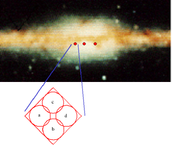
Figure 1.— The position of our fields against the COBE NIR background. From left to right are the MM7B, BW and MM5B fields. MM7B and MM5B each have four overlapping sub-fields as shown in the box.

The signature of the Galactic bar should also be seen in the kinematic distortions of the stellar velocity field, since the orbits are no longer circular, but rather are elongated streams along the bar. The stellar kinematic evidence of bulge triaxiality is still ambiguous. There has been significant work done in the past on the line-of-sight velocities of M and K giants (Rich, 1990; Sharples et al., 1990; Terndrup et al., 1995; Minniti et al., 1992; Habing et al., 2006) and proper motions (Spaenhauer et al., 1992; Sumi et al., 2004; Rattenbury et al., 2007a; Clarkson et al., 2008) in the bulge. But most of these radial velocity observations were limited to the low extinction Baade’s Window ($l\sim 0$°). Häfner et al. (2000) show that measurements in Baade’s Window (BW) alone are insensitive to the effects of triaxiality, and a stronger kinematic signature of the bar will be apparent away from $l=0$°. The ideal observation would be to measure stellar velocity distributions with high S/N for several lines-of-sight (LOS) in the bar. A sample size of $\sim 1000$ stars per LOS would enable the measurements of the higher moments of the velocity distribution and of the average radial velocity shift between the stellar streams in the bar (Mao & Paczyński, 2002; Deguchi et al., 2001). In addition, combining accurate proper motions with these LOS velocities would provide even stronger constraints on the current dynamical models of the Galactic bar.

Further, the ratio of organized stellar streaming motion around the bar to random motion constrains the bar’s angular rotation speed (also called pattern speed) (van Albada & Sanders, 1982). Since bars can interact strongly with dark matter halos, transferring angular momentum into the halo and slowing the bar rotation dramatically (Debattista & Sellwood, 2000), constraining the current pattern speed of the MW bar will provide a bound on the disk to halo mass ratio for the inner Galaxy.

The most recent bulge radial velocity survey by Howard et al. (2008) (also see Rich et al., 2007) measured radial velocities at many positions along the major and minor axes of the bar, obtaining the rotation and velocity dispersion curves. These observations have addressed the crucial problem of measuring kinematics of the bar away from BW. However, their sample size along each LOS is limited to about 100 stars, insufficient to measure the higher moments of the individual velocity distributions or the kinematics of the stellar streams. Our goal in the current investigation is to obtain a large radial velocity sample along several LOS, in order to measure these important quantities.

The basic procedure in Fabry-Pérot (FP) imaging spectroscopy is to obtain a series of narrow-band images, tuning the interferometer over a range of wavelengths covering a spectral feature of interest. The data cube thus produced is analyzed to extract a short portion of the spectrum of each object in the field of view. This spectrum is fit to determine the strength, width and central wavelength of the spectral feature, and the level of the adjacent continuum. If there are many objects of interest within the field of view, the technique can be extremely efficient. FP spectroscopy has traditionally been used to measure emission features in extended objects, and has been highly successful for studying the velocity fields in disk galaxies (e.g. Palunas & Williams, 2000; Zánmar Sánchez et al., 2008) star forming regions (Hartigan et al., 2000), planetary nebula (Sluis & Williams, 2006), and supernova remnants (Ghavamian et al., 2003). It is less common to employ FP techniques to measure absorption spectra, but they have been used to determine the kinematics of stars in a large number of globular clusters (Gebhardt et al., 1994), and the pattern speed of the bar in the early type galaxy NGC 7079 (Debattista & Williams, 2004).

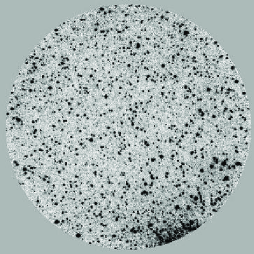
Figure 2.— A Fabry-Pérot image of the Baade’s Window stellar field. The FOV is $4^{\prime}$ and the central wavelength is 8543 Å. The increasing stellar density towards the southwest edge of the field is caused by the bulge globular cluster NGC 6522.

In the present paper we use FP absorption line spectroscopy to obtain radial velocities using the Ca II $\lambda 8542$ line for 2488 Red Clump Giants (RCGs), 339 red giants (M/K type) and 318 disk main sequence stars, towards three LOS in the MW bar: BW and two symmetric offset positions at $(l,b)\simeq(\pm 5.0,-3.5)\arcdeg$ (see Figure 1). This sample is an order of magnitude larger than any previous sample for a given LOS. We also measure equivalent widths of the Ca II $\lambda 8542$ absorption lines that can be used to infer metallicities (e.g. Armandroff & Zinn, 1988) for the late type stars. This will be the subject of a subsequent paper (Paper II) and is discussed only briefly here. In Paper III we will use our measurements for new, more detailed dynamical models of the MW bar.

Table 1Sub-fields observed in the MW bar. Right ascension ($\alpha$) and declination ($\delta$) are from epoch J2000 and $N_{stars}$ indicates the total number of stars (including foreground) obtained from each sub-field.

Field	Date Obs.	$\alpha$	$\delta$	$l(\arcdeg)$	$b(\arcdeg)$	$N_{stars}$
MM5B-a	1996	17:47:24.05	-35:00:21.07	-5.00	-3.47	472
MM5B-b	1997	17:47:40.03	-35:00:34.0	-4.97	-3.52	378
MM5B-c	1999	17:47:20.71	-35:56:52.84	-4.95	-3.43	608
MM5B-d	1997/99	17:47:39.80	-35:56:47.85	-4.92	-3.49	525
BWC-a	1999	18:03:39.70	-29:59:51.2	1.06	-3.93	718
BW1-a	1999	18:02:29.41	-29:49:27.4	1.09	-3.62	359
MM7B-a	1996	18:11:29.61	-25:54:06.6	5.50	-3.46	353
MM7B-b	1997	18:11:44.23	-25:54:26.0	5.52	-3.51	322
MM7B-c	1997/99	18:11:30.32	-25:50:38.5	5.55	-3.44	288
MM7B-d	1999	18:11:44.72	-25:50:33.4	5.58	-3.48	396

2. Observations

Observations were made between 1996 and 1999 using the Rutgers Fabry-Pérot (RFP) system at the f/13.5 Cassegrain focus of the Cerro Tololo Inter-American Observatory (CTIO) 1.5m telescope. The field of view of the RFP was circular with a diameter of $4^{\prime}$. The detector was a Tek 1024 x 1024 pixel CCD, giving an image scale of $0.36\arcsec$ per pixel. Typical seeing was in the range of $1\arcsec-1.5\arcsec$. Each narrow-band exposure was of 900 s duration. A typical image is shown in Figure 2. We observed three LOS: the MM5B field at l = -5°, the MM7B field at l = +5°, and BW. There are four overlapping subfields in each of the MM5B and MM7B fields, as shown in Figure 1, and two sub-fields in BW. Table 1 lists the location of each sub-field and the total number of stars obtained per field. The choice and nomenclature of the fields was motivated by the OGLE survey (Udalski et al., 1992), which provides us with excellent I and V band stellar photometry. In total we obtained $\sim 4400$ stellar spectra.

We chose to observe the Ca II $\lambda 8542$ spectral line. The calcium triplet (8498.02 Å, 8542.09 Å  and 8662.14 Å) is one of the strongest near-infrared spectral features in late-type stars like the RCGs. The triplet arises from the transition between the two levels of $3^{2}\textrm{D}$ and the two levels of $4^{2}\textrm{P}$ in Ca II. The temperature of the bulk of the ISM is not high enough to excite Ca II to the $3^{2}\textrm{D}$ state, and therefore no contamination from the foreground ISM is expected. The 8542 Å line is the strongest of the triplet and falls in a wavelength region where the night sky is relatively free of strong terrestrial emission lines.

We used a medium-resolution etalon with a spectral response function that is well fit by a Voigt function with a FWHM of 4 Å, equivalent to approximately 140 km s^-1 at 8500 Å. We typically scanned a range of $8530-8555$ Å with wavelength steps of 1 Å. The FP images are not monochromatic, because the rays from off-axis points pass through the collimated beam at an angle, making the passband shift to the blue towards the edge of the field. The scanning range was sufficient to compensate for the 4Å center-to-edge gradient by including extra images at the red end of the scan. The resulting spectra allowed measurement of the central wavelength of the line with high precision (5 – 10 km s^-1).

This project was plagued by bad weather and technical difficulties with the instrument and telescope, requiring a significantly longer period of time to acquire the data than expected. During two of the nights in the 1997 run the instrument shutter malfunctioned, affecting the data for sub-fields MM5B-b and MM7B-b, which upon reduction showed large deviations in kinematics compared to the neighboring fields that overlap with them. For this reason we excluded these two fields from our analysis. Because of time constraints only 18 images were obtained for the BW1-a field with heavy obscuration from clouds for half of them, and hence we also excluded this field. These exclusions brought the total sample size down to 3360 stars from seven sub-fields, of which 3144 are used in our kinematic analysis.

We calibrated the wavelength response of the system with several lines around 8542 Å from a neon spectral lamp. The complete calibration sequence was done once per observing run, and was stable over the duration of the run (and indeed from year to year). The precision of the wavelength calibration was typically better than $0.05$ Å, corresponding to 1.8 km s^-1at 8500 Å. The zero-point of the wavelength scale was affected by changes in the environmental conditions such as temperature and atmospheric pressure, and was monitored by taking a single neon calibration image once each hour during the observations. The wavelength zero-point for each observation image was determined by interpolation from these hourly calibrations. On images that have night sky lines within their spectral range, we can also use these sky lines to check the zero point. There were two weak OH lines (at 8548.71 Å & 8538.67 Å; Osterbrock & Martel (1992)) that fall within our scanning range. Although these lines had very low S/N, the zero-point we measured from them for a few frames was consistent with the interpolated calibration ring measurement.

3. Data Reduction

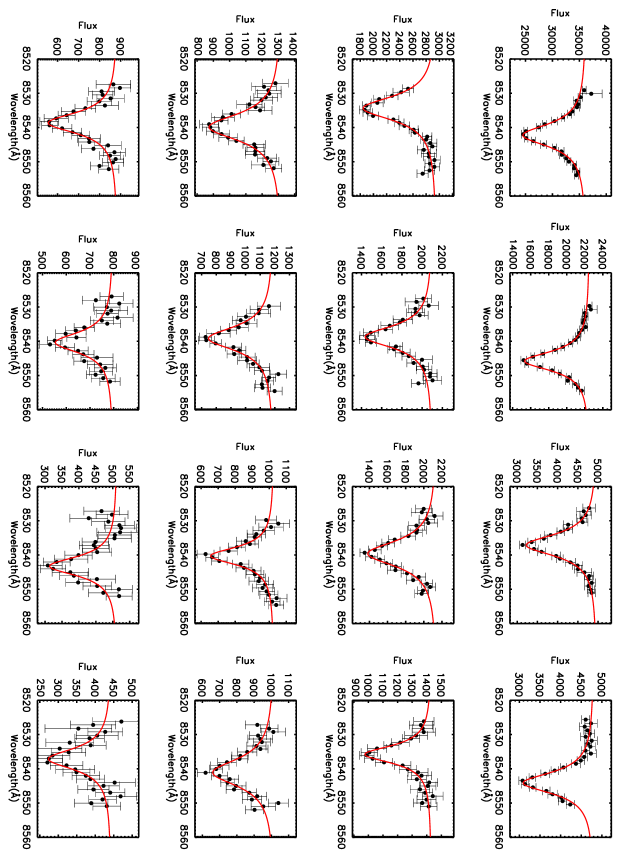
Figure 3.— A sample of the Ca II $\lambda 8542$ spectra for almost the entire brightness range of our sample from I-band magnitude of 11.0 to 16.5. Each data point on the absorption line comes from a single image in the data cube. The solid line is a Voigt fit to the spectrum.

3.1. Fabry-Pérot Photometry

The images in each data cube are overscan corrected, trimmed and bias subtracted using IRAF. To perform photometry on the individual images we use the DAOPHOT stand-alone package by Stetson (1987) that was specially developed to perform crowded field stellar photometry. The task FIND gives the initial centroids of all the stars in the field. After performing the initial aperture photometry using the PHOT task, PSF-based photometry is performed using a quadratically variable PSF, which we found to be especially useful at the edges of the field. We used about 50 – 100 stars per image to determine the PSF. The ALLSTAR task then simultaneously fits all of the stars in the image using the measured PSF to give a star subtracted image, and fluxes and positions for all stars. Because DAOPHOT performs local sky subtraction, the fluxes are not affected by the presence of the weak OH sky lines. DAOPHOT includes the ALLFRAME (Stetson, 1994) program that is particularly useful for reducing a data cube. It simultaneously performs the PSF fitting for all stars in all the images of the cube to derive positions and magnitudes in a self-consistent manner, making use of the geometric transformations between the individual images and photometry information for all images. Because our fields are much less crowded than, for example, a globular cluster, DAOPHOT is able to resolve the stars easily. The final output of DAOPHOT are the centroids, fluxes (in arbitrary units) and flux uncertainty for each star.

3.2. Flux Normalization

In FP absorption line work, it is critically important to account for changes in flux due to variations in atmospheric transmission. This can be significant if the images of a spectral scan were taken over several nights or even in different years, or in non-photometric weather conditions. To measure the image-to-image normalization, we select about 30 high S/N stars uniformly covering the FOV, so that there is a range in velocity and wavelength coverage. We assume that all of these stars have a single dominant absorption line that is well represented by a Voigt function. We fit a Voigt profile to the spectrum of each star, and at each point calculate the ratio of the fit to the observed flux. For each image in the scan, we then calculate the mean and standard deviation of these ratios, using all of the normalization stars for that image. This ratio is the normalization factor for that image. If an image was taken in average transparency conditions, then its normalization factor should be 1.0, within the photometric uncertainty; if the image had lower transparency, the normalization will be greater than unity. We correct the fluxes for each image in the scan using the individual normalization factors. In order to determine the final normalization factors, we re-fit the profile to the normalized data, and iterate the entire process until it converges.

This procedure introduces an additional uncertainty in the flux measurement, which we call the ‘normalization uncertainty’. We combine this in quadrature with the DAOPHOT flux uncertainties. For the highest S/N ($\sim 80$) stars the flux normalization error dominates, while for the majority of stars the DAOPHOT flux error is more important. Since the different normalization stars have a range of velocities, and also because of the center-to-edge wavelength gradient in a FP image, an individual image samples the stars at several different points on the line profile; this avoids “building in” a particular profile shape through the normalization factors. Under photometric conditions, the normalization factors were typically $1.00\pm 0.02$, with uncertainties of $0.002-0.003$. In bad conditions, the worst normalizations were $1.5-2.0$, with uncertainties of $\sim 0.01$. We often re-observed at some of the wavelengths taken under poor conditions, and found excellent agreement between stellar fluxes after normalization.

3.3. Spectroscopy

The Ca II $\lambda 8542$ absorption line profiles with the combined uncertainties are fit with a Voigt function using the Levenberg-Marquardt method of least-squares fitting. The fit gives the central wavelength, continuum level, line strength, and the Gaussian and Lorentzian widths along with their measurement uncertainties. We find that the Gaussian contribution to the shape of the absorption line is negligible for the majority of stars and the line could be fit equally well by fixing the Gaussian width at $10^{-3}$ Å, using essentially a Lorentzian profile. This is because the instrumental profile itself is essentially Lorentzian with a negligible Gaussian core, and the Ca II $\lambda 8542$ line in these stars is strongly saturated with damping wings from collisional broadening. Figure 3 shows a sub-sample of absorption lines covering almost the entire brightness range for our sample from I-band magnitude of 10.0 to 16.5. The Voigt fit is represented by the solid line. For the brightest stars the velocity uncertainties can be as low as 2 km s^-1  and even for the very faint stars we can measure the absorption line adequately well with velocity uncertainties of 20 – 30 km s^-1.

4. Radial Velocities

Figure 4.— The distribution of velocity errors for the MM5B-c field (left panel) and velocity uncertainties as a function of signal-to-noise for the same field (right panel).

Table 4 lists the heliocentric radial velocities and their uncertainties that we measured for our complete sample of 3360 stars with 1605 and 1037 stars at $l=\pm 5$°, respectively, and 718 in BW. The median velocity error for our sample is $\sim 12$ km s^-1. The uncertainties are higher for fainter stars and also in cases where a star has a close or unresolved neighbor. In Figure 4 we show the distribution of velocity errors and the error as a function of S/N for the MM5B-c subfield. The major source of error in the radial velocity measurements comes from the uncertainties in the flux measurements, which include contributions from DAOPHOT and normalization errors. In the case of very high S/N stars in the best seeing sub-fields like MM5B-c and BWC-a (with lower normalization errors) the velocity errors can be as small as 2 – 5 km s^-1.

To check if the velocity errors obtained from our Voigt fitter are reasonable, we carried out Monte Carlo simulations of the data. For each star in our sample, we generated 1000 random realizations of its spectrum by perturbing the fluxes of each point of the Voigt profile fit by the corresponding $1-\sigma$ individual flux uncertainty. We then fit a Voigt function to each of these generated spectra and find that the mean ratio of the error estimate from a single fit to the standard deviation of the velocities from the Monte Carlo fits is about 0.97 for all the fields, indicating that the single fit errors from our Voigt fitter code are reliable.

For the BW LOS, there are nine bulge M/K-giant stars in our work that are also present in the radial velocity samples of Sharples et al. (1990) and Terndrup et al. (1995). The velocity comparison is shown in Figure 5. Our error bars on the horizontal axis are equal to or smaller than the size of the data points. Our velocities agree very well with the previous measurements, with a reduced chi-square of 1.02.

We also have two measurements (repeated over 1 – 3 years) of the radial velocities for some stars in the region where the fields at a given LOS overlap with each other. The comparison between the velocities of stars in these overlapping regions is shown in Figure 6 where the vertical axis shows the velocity difference divided by the $1\sigma$ error bars ($\Delta$). The dashed, dotted and dot-dashed lines show the $1\sigma$, $2\sigma$ and $3\sigma$ limits respectively. The stars at the very edge of the field in the overlapping regions may not show up in every image taken in the scan of that field, so they are not included in this comparison. There is also a 10% chance for a foreground disk main sequence star to be a spectroscopic binary which may result in velocity variations of $\lesssim 30$ km s^-1 (Duquennoy & Mayor, 1991). We find three such examples of foreground stars with large velocity differences in the overlapping regions, and these three stars are omitted from Figure 6. The comparison for the MM5B overlapping regions has a reduced chi-square of $\lesssim 1$. There is one additional star (not foreground) in each of the two overlapping regions of the MM7B fields that has a deviation of more than $3\sigma$, inflating the reduced chi-square for these fields. We don’t have a clear explanation for the deviations in these two cases except that they could be spectroscopic binaries in the bulge. The reduced chi-square for all the stars in the MM7B fields is 1.6; excluding the two outliers reduces chi-square to 1.06.

For most of the stars in the overlapping region we list the weighted mean velocity and errors in Table 4. For the faintest stars from the overlapping regions, we use the velocity from only the field with the best image quality, where the fit to the absorption line was significantly better than the other field. The comparison with previous work, and in the overlapping regions, indicates that our velocity measurements are repeatable and reliable. The velocity uncertainty of less than 30 km s^-1 is small compared to the velocity dispersion of the stars in the bar, and will have no effect on our conclusions.

Figure 5.— Radial velocities of 9 stars in common between this work and previous measurements by Sharples et al. (1990) (squares) and Terndrup et al. (1995) (circles).

5. Photometry and Astrometry

We use photometric information to distinguish between the foreground disk stars, bulge red giants and bulge RCGs. Since our observed fields are coincident with the OGLE survey, we have precision (1 – 2%) V and I band photometry and astrometry (Szymanski, 2005). Unfortunately, the fields MM7B-d and a quarter of MM7B-c fell outside the OGLE field. Photometric observations for these fields were obtained with the 1-m telescope at the South African Astronomical Observatory (SAAO). Reduction of these data using the IRAF photometry package gives V and I band magnitudes with an accuracy of 5% – 10%.

There are some stars in our sample that have no OGLE or SAAO photometry. For these stars we use the FP measurement of the continuum level of the Ca II $\lambda 8542$ absorption line to estimate I-band magnitudes. To check the accuracy of these FP I-band magnitudes we use all the stars in the MM7Bc field where we have both OGLE and SAAO photometry. We determine the zero point of the FP I-band magnitudes from the OGLE photometry for these stars. We compare them to the OGLE and the SAAO magnitudes to find that they are surprisingly consistent with differences $\lesssim 10\%$. These FP I-band magnitudes are used to exclude foreground stars as discussed in section 6. Comparison with the much deeper OGLE survey shows that our sample of RCGs in the bar is essentially complete. Table 4 lists the astrometry and photometry. The photometry source (OGLE, SAAO or FP) is indicated in the last column. The astrometry for all fields comes from OGLE except for the field MM7B-d where the source is the Digitized Sky Survey.

6. Selections from the Color-Magnitude Diagram

The color-magnitude diagram (CMD) is shown in Figure 7 for the MM5B field with 1605 stars. We chose to show the CMD for this particular LOS since it has the largest number of stars and also has OGLE photometry for all them. The CMDs for the other two LOS look almost identical. Paczynski et al. (1994) discuss various parts and features of the BW CMD using the photometry of about $3\times 10^{5}$ stars from the OGLE project. We discuss in brief these features and their selection limits in the $(I_{0},(V-I)_{0})$ plane to be used in our analysis.

Figure 6.— Repeated radial velocity measurements of stars in the overlapping regions of the sub-fields of MM5B and MM7B.

The first feature is a distinct red clump, marked by the red points. These RCGs are very useful candidates for studying the kinematics of the bar. They are basically metal-rich counterparts of the horizontal branch stars burning helium in their cores and hydrogen in their envelopes. Their intrinsic luminosity distribution is very narrow and has a weak dependence on metallicity and age, making them excellent distance indicators (Paczynski & Stanek, 1998). They are bright and numerous in the inner galaxy and are located in the region of CMD that is least contaminated by disk stars (Stanek et al., 1994).

Our selection limits for RCGs towards all three LOS are $(I_{0},(V-I)_{0})=(13.0-15.5,0.5-1.4)$, corrected for the extinction ($A_{I}$) and reddening ($E_{V-I}$) values from Sumi (2004). This I-band limit corresponds to a distance range of about 5.5 – 13 kpc for intrinsic red clump magnitude $M_{I}=-0.28\pm 0.20$ (Paczynski & Stanek, 1998). Stanek et al. (1997) used a slightly different selection criteria for OGLE RCGs where they define extinction independent I-band magnitudes. The effect of these two different selection methods on the overall kinematics of the RCGs is negligible, with changes in the mean radial velocity and dispersion of about 0.75 km s^-1  and 1.15 km s^-1  respectively. The latter selection also gives 2% fewer stars at $l=\pm 5$°and 10% fewer stars in BW. We have also investigated the effect of varying the brighter end of the I-band selection limit from 13.0 – 13.6 magnitudes, which produced negligible changes to the mean velocity and dispersion ($\sim 0.5$ km s^-1). The effects of different selection criteria for RCGs will be more significant when modeling the data (subject of paper III), where it will be investigated in greater detail.

About 210 stars at $(l,b)=(\pm 5.0,-3.5)$°and 39 in BW have only I-band photometry. Without color information it is not possible to distinguish them from the foreground disk stars (blue points in Figure 7). If we apply only I-band cuts then the maximum difference in the kinematics between including or excluding these stars without color information is about 1.3 km s^-1  in mean velocity and 0.6 km s^-1  in dispersion. The 2MASS point source catalogue has J, H and K band photometry for our lines of sight. We found J-K colors for 60% of these stars with no V-I color information. The J-K colors confirmed that after applying the I-band or distance cut about 96% of these stars were RCGs. By analyzing the field MM7B-c, where 99% of the sample has complete V and I band photometry, we find that the contamination due to lack of color information is $\sim 14\%$, after applying the I-band or distance cut. This amounts to contamination by only 11 stars at $l=\pm 5$°and 2 stars in BW. These numbers are negligible compared to the overall sample size and will have little effect on the kinematics. Thus we include these stars (with just the I-band limits) in our final sample that will be used to measure bar kinematics, which now has a total of 1193 RCGs at $(l,b)=(-5.0,-3.5)$°, 738 at $(l,b)=(5.5,-3.5)$°and 557 in BW.

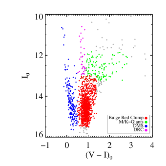
Figure 7.— Extinction-corrected color-Magnitude diagram for the MM5B LOS shows a distinct red clump (red dots). The disk main sequence and the M/K – giants are shown in blue and green dots respectively. We measure the radial velocity of every star in the diagram.

The region marked by the green points at roughly $(I_{0},(V-I)_{0})=(11.8-13.25,0.5-3.0)$ contains the bulge M/K-giants (Sharples et al., 1990; Terndrup et al., 1995). This is the same M-giant population used in the recent radial velocity survey by Rich et al. (2007). In section 7.2 we use them to make a direct comparison with that study. This sample, measured simultaneously from the same data cube, allows us to compare the kinematics of two different stellar populations in the bar/bulge region.

The feature marked by the blue points at $(I_{0},(V-I)_{0})=(10.0-15.7,-0.3-0.5)$ is formed by the disk main sequence (DMS) stars. The stars in this feature are thought to be associated with the Sagittarius spiral arm located at $\sim 2$ kpc from the Sun (Paczynski et al., 1994; Ng et al., 1996). We have radial velocities of about 350 stars in this region over three LOS. This feature and its possible association with the Sagittarius arm is discussed in section 7.3.

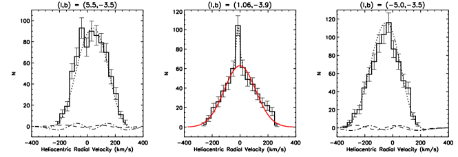
Figure 8.— Stellar radial velocity distribution for three LOS in the bar. Right and Left panel: the dotted line is the Gauss-Hermite fit with $h_{3}$ and $h_{4}$ moments shown by dashed and dot-dashed lines respectively. Middle panel: the dotted line is double Gaussian with a narrow component for the globular cluster NGC 6522 and the solid line is the broad component (only) for the Galactic bar/bulge.

Finally, the feature at $(I_{0},(V-I)_{0})=(10.0-13.0,0.5-0.9)$ on the CMD marked by the magenta points consists of the disk red clump giants spread over a distance of about 1.0 – 4.0 kpc. We had just enough stars in our sample along this LOS to detect this feature and measure its kinematics. The FP imaging spectroscopy has allowed us to measure simultaneously the kinematics of all these features, providing a powerful and reliable way to look for differences between the various stellar populations in a consistent manner.

7. Kinematics

7.1. Kinematics of Red Clump Giants in the Bar: Measurement of $h_{3}$ and $h_{4}$

The large size of our sample allows us to measure, for the first time, the higher moments of the velocity distribution along our three LOS. We fit a Gauss-Hermite series to the velocity distribution (Gerhard, 1993; van der Marel & Franx, 1993) of RCGs to extract the four velocity moments – mean line of sight velocity ($<V_{\textrm{los}}>$), line-of-sight velocity dispersion ($\sigma_{\textrm{los}}$), asymmetry of the distribution ($h_{3}$), and flatness of the distribution ($h_{4}$) – using a maximum likelihood estimator (MLE). An advantage of using the MLE is that it corrects for the individual velocity errors that can broaden the width of the distribution. We use the MLE code developed by Glenn Van de Ven (private communication; see van de Ven et al. (2006) for more details) to fit a Gauss-Hermite series to our velocity distributions and to determine the velocity moments. The code gives a robust measurement of the uncertainties of each moment in two ways. The bootstrap method randomly draws from the observed velocity distribution with replacement (see Sect. 15.6 of Press et al., 1992); this gives the maximum possible errors of the parameters. The Gaussian randomization (GR) method randomly draws velocities from an intrinsic Gaussian distribution with a given mean and dispersion that is broadened by velocity errors randomly drawn from the observed velocity error distribution (see Appendix B of van de Ven et al., 2006). GR gives reliable estimates if the individual errors are not underestimated, which we believe is the case with our analysis. Finally, the code uses the biweight statistic to measure just the first two velocity moments ($<V_{\textrm{los}}>$ and $\sigma_{\textrm{los}}$) and their uncertainties; these are the appropriate measures to compare with previous investigations that had too few stars to reliably determine the higher moments.

MM5B-a and MM5B-c have identical kinematics and can be combined into a single field MM5B-(a+c). MM5B-d is at the same LOS and overlaps with the MM5B-c sub-field but has a mean velocity that is offset by 13 km s^-1 (i.e. about a $2\sigma$ deviation). The dispersions in all three sub-fields however agree within the $1\sigma$ errors. For this reason we measure the velocity moments at $l=-5.0$° using both MM5B-(a+c) as well as the three sub-fields combined MM5B-(a+c+d). There are no significant differences in the kinematics of sub-fields MM7B-a, MM7B-c and MM7B-d, so they are combined into a single field MM7B-(a+c+d). The velocity distributions for MM5B-(a+c) and MM7B-(a+c+d) are shown in the left and right panel of Figure 8. The dotted line is the Gauss-Hermite fit with the $h_{3}$ and $h_{4}$ moments represented by the dashed and dot-dashed lines respectively. Table 5 lists the velocity moments along with their uncertainties. Our large sample size allows us to measure $<V_{\textrm{los}}>$ and $\sigma_{\textrm{los}}$ with high accuracy. As expected, in Galactocentric coordinates $<V_{\textrm{los}}>$ has equal amplitude of about $\pm 63$ km s^-1 at $l=\pm 5$°, respectively. The $h_{4}$ moment is significantly non-zero while the $h_{3}$ is consistent with zero. Our high S/N velocity distributions show no sign of cold kinematic features that could be related to disrupted satellites, as suggested by Rich et al. (2007).

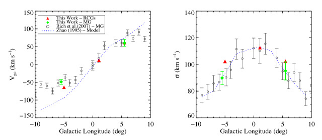
Figure 9.— Comparison of the kinematics (in galactocentric frame) of RCGs (red triangles) and M-giants (green diamonds) from our sample to Rich et al. (2007) data (open circles) and Zhao (1996) model (blue dashed line)

The analysis of the BW velocity distribution (middle panel) is slightly complicated by the presence of stars from the bulge globular cluster NGC 6522, the outskirts of which extend into the southwest edge of our field (see Figure 2). The spike at the center of the BW velocity distribution (shown in Figure 8 middle panel) is caused by the stars that are part of this cluster. To extract kinematics we fit a double Gaussian (broad for the bulge and narrow for NGC 6522) to this distribution. The narrow Gaussian has a mean velocity of $-14.67\pm 3.77$ km s^-1 and dispersion of $7.9\pm 2.82$ km s^-1 ; consistent with previous measurements for NGC 6522 of $-10.3\pm 1.6$ km s^-1 and $7.3^{+3.5}_{-2.0}$ km s^-1  respectively (Dubath et al., 1997). The dotted line in Figure 8 shows the double gaussian fit to the distribution and the solid line is the broad component representing the bulge velocity distribution. We also fit a Gauss-Hermite series to this distribution and list the values in Table 5, although this measurement is most probably affected by the presence of the spike at the center. Since this is the most heavily studied LOS, there are several measurements of the kinematics in BW for comparison. Our values of the mean line-of-sight velocity and dispersion are in excellent agreement with all previous measurements of the kinematics in BW such as Mould (1983) ($<V_{\textrm{los}}>=-10\pm 19$ km s^-1, $\sigma_{\textrm{los}}=113\pm 11$ km s^-1), Sharples et al. (1990) ($<V_{\textrm{los}}>=4\pm 8$ km s^-1, $\sigma_{\textrm{los}}=113^{+6}_{-5}$ km s^-1), Rich (1990) ($<V_{\textrm{los}}>=-13\pm 12$ km s^-1, $\sigma_{\textrm{los}}=111\pm 8$ km s^-1), Terndrup et al. (1995) ($<V_{\textrm{los}}>=-8\pm 6$ km s^-1, $\sigma_{\textrm{los}}=110\pm 10$ km s^-1) and Rich et al. (2007) ($<V_{\textrm{los}}>=-1.1\pm 12.9$ km s^-1, $\sigma_{\textrm{los}}=110.2\pm 9.1$ km s^-1).

7.2. Kinematics of M-giants

Our measurements of the kinematics of M-giants (in the heliocentric coordinate system) are listed in Table 2. We do not tabulate the measurements for BW since the globular cluster M-giants dominate the already small sample, and are difficult to separate from the bulge population, making the measurement unreliable. In Figure 9 we compare the kinematics of the bulge RCGs and M-giants from our sample with that of Rich et al. (2007) M-giants and Zhao (1996) (Zhao hereafter) model. We find that the radial velocities of the RCGs and M-giants stars agree well with each other and with the Rich et al. (2007) measurements. However the LOS dispersion for our M-giant sample (green diamonds) is systematically lower than the RCGs (red triangles), and is consistent with the velocity dispersion of Rich et al. (2007) M-giants (black circles). Note that the higher dispersion of the RCGs in our sample is not because they are fainter and thus have somewhat larger velocity uncertainties. The MLE method we use removes the effects of the uncertainties from the estimate of the dispersion. In any event, to produce the difference between the M-giant and the RCG dispersion would require addition in quadrature of 40 – 50 km s^-1  compared to the uncertainties of 10 – 25 km s^-1.

The blue dashed line in Figure 9 is the prediction from Zhao’s model. The bar in this model rotates faster than the observed rotation curve at greater longitudes. According to Zhao and Rich et al. (2007) this rapid rotation is due to a lack of retrograde orbits in the model. But adding retrograde orbits will increase the $\sigma_{\textrm{los}}$ of the model, which may then agree with the dispersion of RCGs rather than that of the M-giants.

Table 2Kinematics of bar M-giants and disk main sequence stars

LOS	$<V_{\mathrm{los}}>$	$\sigma_{\textrm{los}}$	N
	($\mathrm{km\,s^{-1}}$)	($\mathrm{km\,s^{-1}})$
M-giants
(-5.0, -3.5)	$-37.2\pm 6.9$	$89.9\pm 4.9$	171
(5.5, -3.5)	$29.9\pm 9.6$	$95.2\pm 6.8$	98
DMS
(-5.0, -3.5)	$-17.8\pm 4.0$	$45.9\pm 2.8$	134
(1.06, -3.9)	$-3.1\pm 4.8$	$41.3\pm 3.4$	75
(5.5, -3.5)	$0.9\pm 4.3$	$45.7\pm 3.1$	109

Is there really a difference in dispersion between the M-giants and RCGs? One possibility is that the M-giant sample may have more foreground contamination, which could cause the observed decrement in the dispersion. However, our M-giant selection criteria are virtually the same as those of Rich et al. (2007), who argue that contamination is negligible. If the difference is real, then perhaps there is an age difference between the RCGs and the M-giants, with RCG’s being older. Another possibility is that the M-giants represent multiple dynamical populations. But at this point we have no means to distinguish between these or other hypotheses. We plan to obtain more lines-of-sight in the bar using the FP system (Rangwala et al., 2008) on the 10-m Southern African Large Telescope (SALT) (Buckley et al., 2003) to explore this discrepancy further.

7.3. Kinematics of Disk Stars

Our measurements of the kinematics of the DMS stars (blue dots in figure 7) are listed in Table 2. Earlier studies of the Baade’s window CMD (Terndrup et al., 1995; Paczynski et al., 1994; Ng et al., 1996) found an excess of stars within 2.5 kpc of the Sun. They associated this increased stellar density (by a factor $\sim 2$) of DMS stars with the location of the Sagittarius spiral arm at a distance of $\sim 2$ kpc. The simulations performed by Ng et al. (1996) showed this density enhanced feature to consist of some very young stars (0.1 – 2.0 Gyr) that are identified with the recent spiral arm population superimposed on a larger population of young and intermediate age (2.0 – 7.0 Gyr) stars identified with some past spiral arm population. We find the $\sigma_{\textrm{los}}$ to be the same ($\sim$ 45 km s^-1) towards all three LOS. According to the relationship between velocity dispersion and distance from the Galactic center (Lewis & Freeman, 1989), our dispersion corresponds to a position within 3.5 kpc of the Sun. This suggests that the majority of the stars in this feature may belong to the Sagittarius spiral arm population.

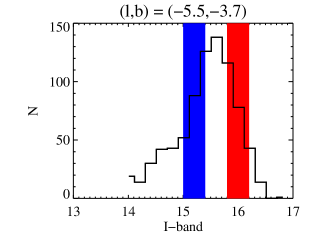
Figure 10.— I-band apparent magnitude distribution of the red clump giants in MM5B field. The two bands show the sample limits for stars on the near and far sides of the bar.

The dispersion of the disk red clump feature (Magenta points on the CMD) is about 53 km s^-1, consistent with the disk kinematics.

8. Radial Streaming Motion

Previous observations have established that the near end of the Galactic bar is in the first Galactic quadrant, i.e., at positive longitudes. Since the stars forming the bar stream in the same sense as the Galactic rotation, for this bar orientation the stars on the near and far side of the bar will have radial velocity components towards and away from us, respectively. The radial velocity difference between these approaching and receding stellar streams depends on the orientation of the bar, among other things. Since RCGs are good distance indicators with a small dispersion in intrinsic luminosity, they can be localized in space and used to measure precisely the velocity shift between the two streams (Mao & Paczyński (2002); MP02 hereafter). This measurement will provide an additional strong constraint on the dynamical models of the Galactic bar, especially its orientation angle.

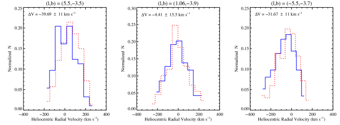
Figure 11.— The radial velocity distribution for the stars in the near and far side samples, shown by the solid and dotted histograms respectively.

MP02 discuss the optimal selection of the bright and faint samples to isolate these stellar streams. We adapt their criteria for the characteristics of our data set, selecting RCGs 0.2 to 0.6 magnitudes brighter and fainter than the peak in the observed luminosity distribution for each field to define the bright (front side) and faint (back side), respectively. Figure 10 illustrates the two samples for the l = -5.0° field, and the details of these bright and faint samples for the three LOS are listed in Table 6. Figure 11 shows the velocity distribution of the near and far side samples. We detect a clear velocity shift of $\sim 35$ km s^-1 in each of $l\simeq\pm 5$° LOS. The velocity shift in BW is much smaller and is consistent with zero. This may be because in BW we are seeing an older spheroidal bulge population superimposed on the bar population, masking this signal. The higher velocity dispersion in BW also indicates that there are higher random motions compared to the streaming motions. Our observed shifts of 35 km s^-1 are much greater than any possible projection effects arising from the Galactic rotation and the location of the near and far samples (1 – 2 km s^-1). This suggests that there are strong non-circular streaming motions associated with the bar. MP02 predicted the difference of the LOS component of the streaming motions between the bright and faint sample to be $\sim 33$ km s^-1  based on the E2 model of Dwek et al. (1995). This predicted shift is consistent with our measurements in the $l=\pm 5$° fields but not in BW. MP02 also discussed the effects of red giant contamination on these shifts and concluded that their presence in the RCG sample could significantly dilute the magnitude of the velocity shifts, so that the actual shifts could be larger than those that we measure.

Deguchi et al. (2001) (see also Deguchi, 2001) used SiO masers in the bar to measure the velocity shifts. They find an average radial velocity difference of $-21\pm 27$ km s^-1 for sources with distances less than 7 kpc compared to those at distances greater than 7 kpc, essentially independent of longitude. While their results agree with our measurements, they suffer from a large (50%) uncertainty in distance and large statistical errors in kinematics (due to a smaller sample size).

As pointed out by Deguchi et al. (2001) most of the dynamical models of the inner galaxy do not predict or even discuss the change in average radial velocity with distance. The dynamical model of Häfner et al. (2000) was one of the first to discuss this in some detail. In their Figures 9 and 10 they plot line-of-sight and proper motion kinematics as a function of distance for four windows, one of which is BW. We have a large enough sample of RCGs to plot LOS average velocity and dispersion as a function of distance in the inner galaxy, which we show in Figure 12. Although we cannot make an exact comparison with Hafner’s predictions for BW since they use a generic selection function for K giants, our data are nonetheless in excellent agreement with their model (open diamonds in Figure 12).

Figure 12.— Line-of-sight radial velocity and dispersion as a function of I-band magnitude (or distance) of the bulge red clump giants for three LOS in the Galactic bar. The vertical dashed line shows the position of the peak magnitude about which the bright and faint samples were measured. Note that these are apparent magnitude not corrected for extinction. The open diamonds show Häfner et al. (2000)’s dynamical model.

9. Equivalent Widths

Table 4 lists the equivalent widths and their uncertainties for our complete sample of 3360 stars. We measured the equivalent widths of Ca II $\lambda 8542$ lines in our sample by integrating the Voigt fit over all wavelengths. Our measurements of mean equivalent width and dispersion for the bulge RCGs are listed in Table 3. The mean equivalent width ($<\mathrm{EW}>$) and its dispersion decrease on either side of BW similar to the LOS velocity dispersion. Because the Ca II $\lambda 8542$ line is a good proxy for metallicity (Armandroff & Zinn, 1988), the gradient in the mean equivalent width may imply a gradient in metallicity (Frogel, 1988; Minniti et al., 1995) along the Galactic bar. We also find that the mean EW of the DMS stars is about 25% lower than the bulge RCGs, which is consistent with a bulge that is more metal rich than the solar neighborhood. This has been the consensus of many previous studies in BW, for example Rich (1988). The factors affecting the measurement of FP equivalent widths and inferring [Fe/H] using the calcium infrared triplet method is addressed in detail in Paper II. For recent work on the metallicity of the Galactic bulge see Fulbright et al. (2006); Minniti & Zoccali (2008).

10. Discussion and Conclusions

Table 3Mean equivalent width and dispersion for the Ca II $\lambda 8542$ line in the bar RCGs

LOS	$<\mathrm{EW}>$	$\sigma_{\mathrm{EW}}$	N
	Å	Å
(-5.0,-3.5)	$3.68\pm 0.04$	$0.46\pm 0.04$	804
(1.1,-3.9)	$3.86\pm 0.05$	$0.68\pm 0.04$	557
(5.5,-3.5)	$3.28\pm 0.04$	$0.48\pm 0.04$	738

In this paper we have presented measurements of the Ca II $\lambda 8542$ absorption line using Fabry-Pérot imaging spectroscopy. This work shows the strength and reliability of this technique in measuring radial velocities for a large sample of stars with I-band magnitudes ranging from 10.0 – 16.5. Past investigations have mostly used red giants to study the bar’s stellar kinematics. Our work is the first to measure the kinematics of red clump giants, which are more numerous in the inner galaxy than the M and K giants. The main focus of this paper is to present the data and preliminary interpretations, but full interpretation will only be possible with extensive modeling that we will present in Paper III.

We obtained radial velocities for three LOS in the MW bar that include two offset positions at $l\simeq\pm 5$°and the central field of BW. The large sample size enabled high precision measurements of the first four moments of the velocity distributions for the first time. The symmetric moment $h_{4}$ is significantly non-zero, and its negative value indicates that the distributions are flat-topped rather than peaked. This seems consistent with a model of the bar with stars in elongated orbits forming two streams at different mean radial velocities, broadening and flattening the total distribution. Because our sample of bar RCGs is essentially complete, the continuity equation suggests that the number of stars in the two streams should be the same. Table 6 shows that this is the case within the Poisson noise. We then expect no asymmetry in the velocity distribution function, and our measures of $h_{3}$ are indeed consistent with zero.

When we divide our sample into bright and faint samples we detect a clear kinematic signature of streaming motions about the bar. The stellar streams have velocity difference of about 35 km s^-1 at $l=\pm 5$°. There is no indication of these streams in BW, perhaps because they are masked by a spheroidal bulge component. The larger velocity dispersion in BW is consistent with this interpretation. Our large sample size allows us to take the first step towards measuring the LOS kinematics as a function of apparent magnitude (or distance) using the RCGs. As Häfner et al. (2000) points out, these measurements can provide powerful constraints on dynamical models of the inner Galaxy. With larger data sets it will be possible to detect the transition from disk to bar, and measure the bar’s thickness.

The technique of FP imaging spectroscopy has allowed us to measure the radial velocities samples that are an order of magnitude larger (at individual LOS) than previous studies. This large sample allows us to determine the kinematics of various stellar populations: bar RCGs, bar M-giants and the disk main sequence stars. Our measurements show that the RCG and M-giant populations have the same $<V_{\textrm{los}}>$ but their dispersions differ by about 10 km s^-1. The kinematics of the DMS population suggests that most of these stars belong to the Sagittarius spiral arm.

In addition to the kinematic measurement, we have used the FP spectra to measure the Ca II $\lambda 8542$ line strengths. We can use these results to measure the metallicities of the individual stars. Metallicity distributions for several LOS in the bar/bulge can provide strong constraints on the chemical evolution models that can determine the star formation rate, initial mass function, and formation time scale (e.g. Matteucci & Romano, 1999; Zoccali et al., 2007) for the inner Galaxy. Our measurements indicate a gradient in mean and dispersion of equivalent width as a function of Galactic longitude, and a clear difference in the mean line strengths between the disk and bulge/bar. The metallicity measurements will be the subject of Paper II.

Motivated by the success of this project, we plan to use the FP system on the 10-m class SALT to obtain a much more extensive determination of the kinematics and metallicity of stars in the inner Galaxy. SALT’s much greater aperture and larger FOV will enable us to measure $\gtrsim 2000$ stars along a single LOS in an hour of observing time. We will investigate at least 10 LOS along the major axis of the bar, obtaining 15000 – 20000 stellar spectra. This data set will provide the basis for models of the structure and chemical evolution of the Galactic bar and bulge. We can also investigate the long bar suggested by recent Spitzer observations (Benjamin, 2008) and search for hypervelocity stars. This planned increase by another order of magnitude in the size of the data sample will revolutionize the studies of the inner Galaxy.

Table 4Radial Velocities and Equivalent Widths

ID	OGLEID	R.A.	Dec.	$V$	$V_{\textrm{err}}$	EW	EW${}_{\textrm{err}}$	I	V-I	Source
		j2000	j2000	km $\textrm{s}^{-1}$	km $\textrm{s}^{-1}$	Å	Å
BWCa-1	256217	18:03:35.16	-29:58:12.3	-4.49	1.60	4.64	0.17	11.560	2.117	o
BWCa-2	256200	18:03:31.91	-30:00:28.3	-27.71	2.55	2.12	0.12	11.523	3.960	o
BWCa-3	256193	18:03:31.67	-30:00:43.4	-44.86	1.91	4.55	0.19	11.730	2.522	o
BWCa-4	402256	18:03:43.52	-30:01:46.1	-17.77	1.70	4.34	0.15	11.733	1.358	o
BWCa-5	256201	18:03:30.78	-30:00:27.9	92.33	2.41	3.79	0.18	12.241	2.702	o
BWCa-6	256199	18:03:32.87	-30:00:31.4	9.84	3.60	2.42	0.20	12.098	0.710	o
BWCa-8	402258	18:03:45.27	-30:01:32.5	-74.90	3.48	2.94	0.22	12.214	3.876	o
BWCa-9	–	18:03:36.34	-30:01:50.2	-20.10	3.03	3.80	0.23	12.020	–	f
BWCa-11	244433	18:03:34.54	-30:01:37.6	32.20	3.41	1.20	0.11	12.229	4.566	o
BWCa-12	412692	18:03:38.98	-29:58:25.9	-38.04	2.72	5.65	0.31	12.215	2.595	o
BWCa-13	423223	18:03:41.96	-29:57:49.1	-70.86	2.80	4.07	0.25	12.289	2.120	o
BWCa-15	412682	18:03:38.18	-30:00:51.2	-16.60	2.91	4.07	0.23	12.467	1.912	o
BWCa-16	412681	18:03:38.24	-30:00:59.7	67.05	2.41	4.64	0.23	12.476	2.346	o
BWCa-19	412690	18:03:36.96	-29:58:47.1	-58.58	2.45	6.04	0.31	12.483	2.094	o
BWCa-20	256196	18:03:33.66	-30:00:36.1	-24.73	2.47	3.46	0.20	12.579	1.894	o
BWCa-21	412685	18:03:42.64	-30:00:06.5	131.70	3.01	4.69	0.32	12.493	2.927	o
BWCa-22	402257	18:03:37.71	-30:01:34.0	-15.85	2.90	3.79	0.22	12.637	2.040	o
BWCa-23	412683	18:03:47.96	-30:00:38.1	-17.18	3.30	4.40	0.32	12.627	2.948	o
BWCa-27	412719	18:03:39.69	-29:58:47.5	-108.48	3.33	6.48	0.35	12.787	2.576	o
BWCa-28	412708	18:03:49.05	-29:59:35.0	-7.34	2.95	5.23	0.35	12.905	2.475	o
BWCa-29	256222	18:03:34.70	-30:01:15.7	-18.07	3.08	3.48	0.23	12.923	1.883	o
BWCa-30	412702	18:03:37.64	-30:00:26.0	-45.72	6.02	3.66	0.41	12.877	0.925	o
BWCa-32	256236	18:03:34.96	-29:59:48.6	-76.35	5.27	4.78	0.45	12.982	3.493	o
BWCa-33	412727	18:03:45.61	-29:58:12.0	-132.32	3.95	4.81	0.40	13.174	2.579	o
BWCa-34	412711	18:03:41.51	-29:59:20.3	-134.86	3.59	4.75	0.26	13.081	2.852	o
BWCa-35	256235	18:03:30.56	-29:59:51.0	44.72	3.22	4.07	0.29	13.173	2.307	o
BWCa-36	256238	18:03:32.78	-29:59:39.1	143.70	2.71	4.15	0.27	13.132	2.736	o
BWCa-38	412728	18:03:42.44	-29:58:10.6	-168.91	3.82	5.29	0.34	13.205	2.625	o
BWCa-39	412712	18:03:47.60	-29:59:15.4	-65.47	3.57	5.50	0.38	13.223	2.865	o
BWCa-40	412718	18:03:38.12	-29:58:58.3	3.29	3.78	5.35	0.39	13.150	2.474	o
BWCa-42	412732	18:03:37.09	-29:57:56.3	4.77	3.54	2.35	0.22	13.133	1.571	o
BWCa-43	412724	18:03:39.04	-29:58:28.0	-153.07	4.33	5.49	0.39	13.173	1.917	o
BWCa-44	412704	18:03:38.05	-30:00:10.2	-61.60	4.52	3.80	0.27	13.141	1.419	o
BWCa-45	412716	18:03:47.48	-29:59:06.4	110.99	2.89	4.14	0.28	13.309	2.530	o
BWCa-46	412699	18:03:46.37	-30:00:47.9	-130.64	3.93	4.99	0.36	13.333	2.210	o
BWCa-47	412720	18:03:45.08	-29:58:46.3	89.38	3.35	4.34	0.31	13.284	2.242	o
BWCa-48	402288	18:03:40.62	-30:01:46.0	-10.80	4.33	3.03	0.30	13.377	1.751	o
BWCa-49	412729	18:03:39.95	-29:58:07.8	-102.93	4.34	4.77	0.37	13.295	1.956	o
BWCa-50	256226	18:03:36.45	-30:00:39.8	-13.72	3.74	5.04	0.39	13.311	2.713	o

Note. — Table 4 is published in its entirety in the electronic edition of the Astrophysical Journal. A portion is shown here for guidance regarding its form and content.

Table 5Heliocentric kinematics of the red clump giants for three LOS in the Milky Way bar.

Method	$<V_{\textrm{los}}>$	$\sigma_{\textrm{los}}$	$h_{3}$	$h_{4}$
MM5B-(a+c); $(l,b)=(-5.0,-3.5)$; $N_{\textrm{stars}}=804$
Likelihood	$-54.15\pm 3.66\,(\pm 6.14)$	$101.72\pm 0.66\,(\pm 0.80)$	$-0.030\pm 0.017\,(\pm 0.034)$	$-0.032\pm 0.008\,(\pm 0.017)$
Biweight	$-52.56\pm 0.60\,(\pm 3.85)$	$102.30\pm 1.25\,(\pm 2.50)$	$\cdots$	$\cdots$
MM5B-(a+c+d); $(l,b)=(-5.0,-3.5)$; $N_{\textrm{stars}}=1193$
Likelihood	$-56.46\pm 1.84\,(\pm 4.48)$	$102.04\pm 0.09\,(\pm 0.28)$	$-0.018\pm 0.007\,(\pm 0.018)$	$-0.031\pm 0.005\,(\pm 0.012)$
Biweight	$-58.57\pm 0.48\,(\pm 3.35)$	$101.46\pm 1.21\,(\pm 2.03)$	$\cdots$	$\cdots$
MM7B-(a+c+d); $(l,b)=(5.5,-3.5)$; $N_{\textrm{stars}}=738$
Likelihood	$35.73\pm 7.20\,(\pm 9.44)$	$102.40\pm 0.15\,(\pm 0.31)$	$-0.016\pm 0.031\,(\pm 0.043)$	$-0.047\pm 0.022\,(\pm 0.026)$
Biweight	$30.73\pm 0.58\,(\pm 3.89)$	$102.38\pm 1.21\,(\pm 2.39)$	$\cdots$	$\cdots$
BWC-a; $(l,b)=(1.06,-3.9)$; $N_{\textrm{stars}}=557$
Likelihood	$4.32\pm 0.26\,(\pm 5.21)$	$110.29\pm 0.36\,(\pm 0.73)$	$-0.031\pm 0.011\,(\pm 0.019)$	$-0.035\pm 0.009\,(\pm 0.017)$
BW (B)	$-1.01\pm 5.42$	$112.62\pm 3.41$	$\cdots$	$\cdots$
NGC 6522 (N)	$-14.67\pm 3.77$	$7.9\pm 2.82$

Note. — There are two types of errors for the velocity moments: Gaussian randomization and bootstrap (in parenthesis).

For BW kinematics the B and N stand for the broad and narrow Gaussian components.

Table 6Radial streaming motions.

LOS	Ipeak	$\langle V_{\textrm{bright}}\rangle$	$N_{\textrm{bright}}$	$\langle V_{\textrm{faint}}\rangle$	$N_{\textrm{faint}}$	$\Delta V$
(l,b)		(km s-1)		(km s-1)		(km s-1)
$(+5.5,-3.5)$	15.4	$13.57\pm 7.5$	186	$52.90\pm 8.3$	140	$-39.69\pm 11.2$
$(+1.06,-3.9)$	15.2	$-7.05\pm 11.3$	94	$-2.64\pm 10.7$	109	$-4.41\pm 15.5$
$(-5.0,-3.5)$	15.6	$-73.48\pm 8.1$	174	$41.81\pm 8.1$	167	$-31.67\pm 11.5$

References

- Alcock et al. (2000) Alcock, C., Allsman, R. A., Alves, D. R., Axelrod, T. S., Becker, A. C., Bennett, D. P., Cook, K. H., Drake, A. J., Freeman, K. C., Geha, M., Griest, K., Lehner, M. J., Marshall, S. L., Minniti, D., Nelson, C. A., Peterson, B. A., Popowski, P., Pratt, M. R., Quinn, P. J., Stubbs, C. W., Sutherland, W., Tomaney, A. B., Vandehei, T., & Welch, D. L. 2000, ApJ, 541, 734
- Armandroff & Zinn (1988) Armandroff, T. E., & Zinn, R. 1988, AJ, 96, 92
- Benjamin (2008) Benjamin, R. A. 2008, in Bulletin of the American Astronomical Society, Vol. 40, Bulletin of the American Astronomical Society, 266–+
- Benjamin et al. (2005) Benjamin, R. A., Churchwell, E., Babler, B. L., Indebetouw, R., Meade, M. R., Whitney, B. A., Watson, C., Wolfire, M. G., Wolff, M. J., Ignace, R., Bania, T. M., Bracker, S., Clemens, D. P., Chomiuk, L., Cohen, M., Dickey, J. M., Jackson, J. M., Kobulnicky, H. A., Mercer, E. P., Mathis, J. S., Stolovy, S. R., & Uzpen, B. 2005, ApJ, 630, L149
- Binney et al. (1991) Binney, J., Gerhard, O. E., Stark, A. A., Bally, J., & Uchida, K. I. 1991, MNRAS, 252, 210
- Bissantz et al. (2004) Bissantz, N., Debattista, V. P., & Gerhard, O. 2004, ApJ, 601, L155
- Bissantz & Gerhard (2002) Bissantz, N., & Gerhard, O. 2002, MNRAS, 330, 591
- Blitz & Spergel (1991) Blitz, L., & Spergel, D. N. 1991, ApJ, 379, 631
- Buckley et al. (2003) Buckley, D. A. H., Hearnshaw, J. B., Nordsieck, K. H., & O’Donoghue, D. 2003, in Presented at the Society of Photo-Optical Instrumentation Engineers (SPIE) Conference, Vol. 4834, Discoveries and Research Prospects from 6- to 10-Meter-Class Telescopes II. Edited by Guhathakurta, Puragra. Proceedings of the SPIE, Volume 4834, pp. 264-275 (2003)., ed. P. Guhathakurta, 264–275
- Cabrera-Lavers et al. (2008) Cabrera-Lavers, A., Gonzalez-Fernandez, C., Garzon, F., Hammersley, P. L., & Lopez-Corredoira, M. 2008, ArXiv e-prints, 809
- Clarkson et al. (2008) Clarkson, W., Sahu, K., Anderson, J., Smith, T. E., Brown, T. M., Rich, R. M., Casertano, S., Bond, H. E., Livio, M., Minniti, D., Panagia, N., Renzini, A., Valenti, J., & Zoccali, M. 2008, ApJ, 684, 1110
- de Vaucouleurs (1964) de Vaucouleurs, G. 1964, in IAU Symposium, Vol. 20, The Galaxy and the Magellanic Clouds, ed. F. J. Kerr, 195–+
- Debattista & Sellwood (2000) Debattista, V. P., & Sellwood, J. A. 2000, ApJ, 543, 704
- Debattista & Williams (2004) Debattista, V. P., & Williams, T. B. 2004, ApJ, 605, 714
- Deguchi (2001) Deguchi, S. 2001, in Astronomical Society of the Pacific Conference Series, Vol. 228, Dynamics of Star Clusters and the Milky Way, ed. S. Deiters, B. Fuchs, A. Just, R. Spurzem, & R. Wielen, 404–+
- Deguchi et al. (2001) Deguchi, S., Fujii, T., Matsumoto, S., Nakashima, J.-I., & Wood, P. R. 2001, PASJ, 53, 293
- Dubath et al. (1997) Dubath, P., Meylan, G., & Mayor, M. 1997, A&A, 324, 505
- Duquennoy & Mayor (1991) Duquennoy, A., & Mayor, M. 1991, A&A, 248, 485
- Dwek et al. (1995) Dwek, E., Arendt, R. G., Hauser, M. G., Kelsall, T., Lisse, C. M., Moseley, S. H., Silverberg, R. F., Sodroski, T. J., & Weiland, J. L. 1995, ApJ, 445, 716
- Freeman (1996) Freeman, K. C. 1996, in Astronomical Society of the Pacific Conference Series, Vol. 91, IAU Colloq. 157: Barred Galaxies, ed. R. Buta, D. A. Crocker, & B. G. Elmegreen, 1–+
- Freudenreich (1998) Freudenreich, H. T. 1998, ApJ, 492, 495
- Frogel (1988) Frogel, J. A. 1988, ARA&A, 26, 51
- Fulbright et al. (2006) Fulbright, J. P., McWilliam, A., & Rich, R. M. 2006, ApJ, 636, 821
- Gebhardt et al. (1994) Gebhardt, K., Pryor, C., Williams, T. B., & Hesser, J. E. 1994, AJ, 107, 2067
- Gerhard (1993) Gerhard, O. E. 1993, MNRAS, 265, 213
- Gerhard (1999) Gerhard, O. E. 1999, in Astronomical Society of the Pacific Conference Series, Vol. 182, Galaxy Dynamics - A Rutgers Symposium, ed. D. R. Merritt, M. Valluri, & J. A. Sellwood, 307–+
- Ghavamian et al. (2003) Ghavamian, P., Rakowski, C. E., Hughes, J. P., & Williams, T. B. 2003, ApJ, 590, 833
- Habing et al. (2006) Habing, H. J., Sevenster, M. N., Messineo, M., van de Ven, G., & Kuijken, K. 2006, A&A, 458, 151
- Häfner et al. (2000) Häfner, R., Evans, N. W., Dehnen, W., & Binney, J. 2000, MNRAS, 314, 433
- Hartigan et al. (2000) Hartigan, P., Morse, J., Palunas, P., Bally, J., & Devine, D. 2000, AJ, 119, 1872
- Howard et al. (2008) Howard, C. D., Rich, R. M., Reitzel, D. B., Koch, A., De Propris, R., & Zhao, H. 2008, ArXiv e-prints, 807
- Lewis & Freeman (1989) Lewis, J. R., & Freeman, K. C. 1989, AJ, 97, 139
- Liszt & Burton (1980) Liszt, H. S., & Burton, W. B. 1980, ApJ, 236, 779
- Mao & Paczyński (2002) Mao, S., & Paczyński, B. 2002, MNRAS, 337, 895
- Matteucci & Romano (1999) Matteucci, F., & Romano, D. 1999, Ap&SS, 265, 311
- Minniti et al. (1995) Minniti, D., Olszewski, E. W., Liebert, J., White, S. D. M., Hill, J. M., & Irwin, M. J. 1995, MNRAS, 277, 1293
- Minniti et al. (1992) Minniti, D., White, S. D. M., Olszewski, E. W., & Hill, J. M. 1992, ApJ, 393, L47
- Minniti & Zoccali (2008) Minniti, D., & Zoccali, M. 2008, 245, 323
- Mould (1983) Mould, J. R. 1983, ApJ, 266, 255
- Ng et al. (1996) Ng, Y. K., Bertelli, G., Chiosi, C., & Bressan, A. 1996, A&A, 310, 771
- Osterbrock & Martel (1992) Osterbrock, D. E., & Martel, A. 1992, PASP, 104, 76
- Paczynski & Stanek (1998) Paczynski, B., & Stanek, K. Z. 1998, ApJ, 494, L219+
- Paczynski et al. (1994) Paczynski, B., Stanek, K. Z., Udalski, A., Szymanski, M., Kaluzny, J., Kubiak, M., & Mateo, M. 1994, AJ, 107, 2060
- Palunas & Williams (2000) Palunas, P., & Williams, T. B. 2000, AJ, 120, 2884
- Press et al. (1992) Press, W. H., Teukolsky, S. A., Vetterling, W. T., & Flannery, B. P. 1992, Numerical recipes in FORTRAN. The art of scientific computing (Cambridge: University Press, —c1992, 2nd ed.)
- Rangwala et al. (2008) Rangwala, N., Williams, T. B., Pietraszewski, C., & Joseph, C. L. 2008, AJ, 135, 1825
- Rattenbury et al. (2007a) Rattenbury, N. J., Mao, S., Debattista, V. P., Sumi, T., Gerhard, O., & de Lorenzi, F. 2007a, MNRAS, 378, 1165
- Rattenbury et al. (2007b) Rattenbury, N. J., Mao, S., Sumi, T., & Smith, M. C. 2007b, MNRAS, 378, 1064
- Rich (1988) Rich, R. M. 1988, AJ, 95, 828
- Rich (1990) —. 1990, ApJ, 362, 604
- Rich et al. (2007) Rich, R. M., Reitzel, D. B., Howard, C. D., & Zhao, H. 2007, ApJ, 658, L29
- Sellwood & Wilkinson (1993) Sellwood, J. A., & Wilkinson, A. 1993, Reports of Progress in Physics, 56, 173
- Sharples et al. (1990) Sharples, R., Walker, A., & Cropper, M. 1990, MNRAS, 246, 54
- Sluis & Williams (2006) Sluis, A. P. N., & Williams, T. B. 2006, AJ, 131, 2089
- Spaenhauer et al. (1992) Spaenhauer, A., Jones, B. F., & Whitford, A. E. 1992, AJ, 103, 297
- Stanek et al. (1994) Stanek, K. Z., Mateo, M., Udalski, A., Szymanski, M., Kaluzny, J., & Kubiak, M. 1994, ApJ, 429, L73
- Stanek et al. (1997) Stanek, K. Z., Udalski, A., Szymanski, M., Kaluzny, J., Kubiak, M., Mateo, M., & Krzeminski, W. 1997, ApJ, 477, 163
- Stetson (1987) Stetson, P. B. 1987, PASP, 99, 191
- Stetson (1994) —. 1994, PASP, 106, 250
- Sumi (2004) Sumi, T. 2004, MNRAS, 349, 193
- Sumi et al. (2004) Sumi, T., Wu, X., Udalski, A., Szymański, M., Kubiak, M., Pietrzyński, G., Soszyński, I., Woźniak, P., Żebruń, K., Szewczyk, O., & Wyrzykowski, Ł. 2004, MNRAS, 348, 1439
- Szymanski (2005) Szymanski, M. K. 2005, Acta Astronomica, 55, 43
- Terndrup et al. (1995) Terndrup, D. M., Sadler, E. M., & Rich, R. M. 1995, AJ, 110, 1774
- Udalski et al. (1992) Udalski, A., Szymanski, M., Kaluzny, J., Kubiak, M., & Mateo, M. 1992, Acta Astronomica, 42, 253
- van Albada & Sanders (1982) van Albada, T. S., & Sanders, R. H. 1982, MNRAS, 201, 303
- van de Ven et al. (2006) van de Ven, G., van den Bosch, R. C. E., Verolme, E. K., & de Zeeuw, P. T. 2006, A&A, 445, 513
- van der Marel & Franx (1993) van der Marel, R. P., & Franx, M. 1993, ApJ, 407, 525
- Weiner & Sellwood (1999) Weiner, B. J., & Sellwood, J. A. 1999, ApJ, 524, 112
- Zánmar Sánchez et al. (2008) Zánmar Sánchez, R., Sellwood, J. A., Weiner, B. J., & Williams, T. B. 2008, ApJ, 674, 797
- Zhao (1996) Zhao, H. S. 1996, MNRAS, 283, 149
- Zoccali et al. (2007) Zoccali, M., Lecureur, A., Barbuy, B., Hill, V., Renzini, A., Minniti, D., Momany, Y., Gómez, A., & Ortolani, S. 2007, 241, 73