Noise Induced Intermittency in a Superconducting Microwave Resonator

Abstract

We experimentally and numerically study a NbN superconducting stripline resonator integrated with a microbridge. We find that the response of the system to monochromatic excitation exhibits intermittency, namely, noise-induced jumping between coexisting steady-state and limit-cycle responses. A theoretical model that assumes piecewise linear dynamics yields partial agreement with the experimental findings.

Nonlinear response of superconducting RF devices can be exploited for a variety of applications such as noise squeezing Movshovich et al. (1990), bifurcation amplification Siddiqi et al. (2004); Castellanos-Beltran and Lehnert (2007); Tholen et al. (2007) and resonant readout of qubits Lee et al. (2006). Recently we have reported on an instability found in NbN superconducting stripline resonators in which a short section of the stripline was made relatively narrow, forming thus a microbridge Segev et al. (2007a, b). In these experiments a monochromatic pump tone, having a frequency close to one of the resonance frequencies, is injected into the resonator and the reflected power off the resonator is measured. We have discovered that there is a certain zone in the pump frequency - pump amplitude plane, in which the resonator exhibits limit-cycle (LC) response resulting in self-sustained modulation of the reflected power. Moreover, to account for the experimental findings we have proposed a simple piecewise linear model, which attributes the resonator’s nonlinear response to thermal instability occurring in the microbridge Segev et al. (2007c). In spite of its simplicity, this model yields a rich variety of dynamical effects. In particular, as we show below, it predicts the occurrence of intermittency, namely the coexistence of different LC and steady state solutions, and noise-induced jumping between them. In the present paper we study both theoretically and experimentally noise-induced transitions between different metastable responses. We employ a 1D map to find the possible LC solutions of the system and to find conditions for the occurrence of intermittency. Experimentally we present measurements showing both, intermittency between a LC and a steady state, and intermittency between different LCs. A comparison between the experimental results and theory yields a partial agreement.

Intermittency is a phenomenon in which a system response remains steady for periods of time (the laminar phase) which are interrupted by irregular spurts of relatively large amplitude dynamics (the turbulent phase). It arises in certain deterministic systems that are near a bifurcation in which a steady response is destabilized or destroyed Berge et al. (1984). This phenomenon also occurs in noisy systems in which the laminar response has a weak point in its local basin of attraction and is randomly bumped across the basin threshold, and then ultimately reinjected back to the laminar state, and the process repeats. This latter type of bursting behavior, which is relevant to the present system, is observed to occur in many other systems, including Rayleigh-Bnard convection Ecke and Haucke (1989), acoustic instabilities Franck et al. (1999), turbulent boundary layers Stone and Holmes (1989), semiconducting lasers Pedaci et al. (2005), blinking quantum dots Kuno et al. (2000), sensory neurons Longtin et al. (1991) and cardiac tissues Chialvo and Jalife (1990). The presence and level of noise has a significant effect on all such systems, since perturbations affect the triggering of the system out of the laminar phase Eckmann et al. (1981); Haucke et al. (1984). The mean duration times of the laminar phase for a certain class of these systems scales in a manner that depends on the bifurcation parameter and the noise level Sommerer et al. (1991a, b). A special feature of the present system is that it exhibits a very sharp transition between two types of operating states, namely, normal conducting (NC) and superconducting (SC), which is modeled by equations with discontinuous characteristics. While the deterministic behavior of such non-smooth systems (at least of low order) is generally well understood, including local and global bifurcations Bernardo et al. (2007), the effects of noise in such systems has not been considered.

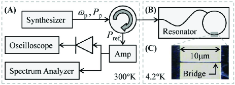
Figure 1: (A) Measurement setup. (B) Schematic layout of the device. (C) Optical microscope image of the microbridge.

The present experiments are performed using the setup depicted in Fig. 1$\left(\mathrm{A}\right)$ Segev et al. (2006). The resonator is stimulated with a monochromatic pump tone having an angular frequency $\omega_{\mathrm{p}}$ and power $P_{\mathrm{p}}$. The power reflected off the resonator is amplified at room temperature and measured by using both, a spectrum analyzer in the frequency domain and an oscilloscope, tracking the reflected power envelope, in the time domain. All measurements are carried out while the device is fully immersed in liquid Helium. A simplified circuit layout of the device is illustrated in Fig. 1$(\mathrm{B})$. The resonator is formed as a stripline ring made of Niobium Nitride (NbN) deposited on a Sapphire wafer Segev et al. (2006); Chang et al. (1987), and having a characteristic impedance of $50\operatorname{\Omega}$. A feedline, which is weakly coupled to the resonator, is employed for delivering the input and output signals. A microbridge is monolithically integrated into the structure of the ring Saeedkia et al. (2005).

The dynamics of our system can be captured by two coupled equations of motion Segev et al. (2007c). Consider a resonator driven by a weakly coupled feedline carrying an incident coherent tone $b^{\mathrm{in}}=b_{0}^{\mathrm{in}}e^{-i\omega_{\mathrm{p}}t}$, where $b_{0}^{\mathrm{in}}$ is constant complex amplitude and $\omega_{\mathrm{p}}$ is the driving angular frequency. The mode amplitude inside the resonator can be written as $Be^{-i\omega_{\mathrm{p}}t}$, where $B\left(t\right)$ is a complex amplitude, which is assumed to vary slowly on a time scale of $1/\omega_{\mathrm{p}}$. In this approximation, the equation of motion of $B$ reads

$$\frac{\mathrm{d}B}{\mathrm{d}t}=\left[i\left(\omega_{\mathrm{p}}-\omega_{0}\right)-\gamma\right]B-i\sqrt{2\gamma_{1}}b^{\mathrm{in}}+c^{\mathrm{in}},$$ (1)

where $\omega_{0}$ is the angular resonance frequency and $\gamma=\gamma_{1}+\gamma_{2}$, where $\gamma_{1}$ is the coupling coefficient between the resonator and the feedline and $\gamma_{2}$ is the damping rate of the mode. The term $c^{\mathrm{in}}$ represents an input Gaussian noise, whose time autocorrelation function is given by $\langle c^{\mathrm{in}}(t)c^{\mathrm{in}\ast}(t^{\prime})\rangle=G\omega_{0}\delta\left(t-t^{\prime}\right)$, where the constant $G$ can be expressed in terms of the effective noise temperature $T_{\mathrm{eff}}$ as $G=\left(2\gamma/\omega_{0}\right)\left(k_{B}T_{\mathrm{eff}}/\hbar\omega_{0}\right)$. The microbridge heat balance equation reads

$$C\frac{\mathrm{d}T}{\mathrm{d}t}=2\hslash\omega_{0}\gamma_{2}\alpha\left|B\right|^{2}-H\left(T-T_{0}\right),$$ (2)

where $T$ is the temperature of the microbridge, $C$ is the thermal heat capacity, $\alpha$ is the portion of the heating power applied to the microbridge relative to the total power dissipated in the resonator ($0\leq\alpha\leq 1$), $H$ is the heat transfer coefficient, and $T_{0}=4.2\operatorname{K}$ is the temperature of the coolant.

Coupling between Eqs. (1) and (2) originates by the dependence of the parameters of the driven mode $\omega_{0}$, $\gamma_{1}$, $\gamma_{2}$ and $\alpha$ on the resistance and inductance of the microbridge, which in turn depend on its temperature. We assume the simplest case, where this dependence is a step function that occurs at the critical temperature $T_{\mathrm{c}}\simeq 10\operatorname{K}$ of the superconductor, namely $\omega_{0}$, $\gamma_{1}$, $\gamma_{2}$ and $\alpha$ take the values $\omega_{0\mathrm{s}}$, $\gamma_{1\mathrm{s}}$, $\gamma_{2\mathrm{s}}$ and $\alpha_{\mathrm{s}}$ respectively for the SC phase $\left(T<T_{\mathrm{c}}\right)$ of the microbridge and $\omega_{0\mathrm{n}}$, $\gamma_{1\mathrm{n}}$, $\gamma_{2\mathrm{n}}$ and $\alpha_{\mathrm{n}}$ respectively for the NC phase $\left(T>T_{\mathrm{c}}\right)$.

Solutions of steady state response to a monochromatic excitation are found by seeking stationary solutions to Eqs. (1) and (2) for the noiseless case $c^{\mathrm{in}}=0$. The system may have, in general, up to two locally stable steady states, corresponding to the SC and NC phases of the microbridge. The stability of each of these phases depend on the corresponding steady states values $B_{\mathrm{s}}=i\sqrt{2\gamma_{1}}b^{\mathrm{in}}/\left[i\left(\omega_{\mathrm{p}}-\omega_{0\mathrm{s}}\right)-\gamma_{\mathrm{s}}\right]$ and $B_{\mathrm{n}}=i\sqrt{2\gamma_{1}}b^{\mathrm{in}}/\left[i\left(\omega_{\mathrm{p}}-\omega_{0\mathrm{n}}\right)-\gamma_{\mathrm{n}}\right]$ [see Eq. (1)]. A SC steady state exists only if $\left|B_{\mathrm{s}}\right|^{2}<E_{\mathrm{s}}$ where $E_{\mathrm{s}}=H\left(T_{\mathrm{c}}-T_{0}\right)/2\hslash\omega_{0\mathrm{s}}\gamma_{2\mathrm{s}}\alpha_{\mathrm{s}}$, whereas a NC steady state exists only if $\left|B_{\mathrm{n}}\right|^{2}>E_{\mathrm{n}}$ where $E_{\mathrm{n}}=H\left(T_{\mathrm{c}}-T_{0}\right)/2\hslash\omega_{0\mathrm{n}}\gamma_{2\mathrm{n}}\alpha_{\mathrm{n}}$. Consequently, four stability zones can be identified in the plane of pump power $P_{\mathrm{p}}\propto\left|b_{0}^{\mathrm{in}}\right|^{2}$ - pump frequency $\omega_{\mathrm{p}}$ (see Fig. 2) Segev et al. (2007c). Two are mono-stable (MS) zones (MS(SC) and MS(NC)), where either the SC or the NC phases is locally stable, respectively. Another is a bistable zone (BiS), where both phases are locally stable. The third is an astable zone (aS), where none of the phases are locally stable.

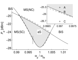
Figure 2: Stability zones in the $\omega_{\mathrm{p}}-P_{\mathrm{p}}$ plane: SC monostable (MS(SC)), NC monostable (MS(NC)), bistable (biS), and astable (aS) (gray colored) zones. The region where a stable LC exists is marked with dashed line. The inset shows the three operating points (A, B and C) at which the measurements and theoretical analysis shown in Fig. 3 and 4 are done. The following parameters were used in the numerical simulation: $\omega_{0\mathrm{s}}/2\pi=3.49\operatorname{GHz}$, $\gamma_{1\mathrm{s}}=0.025\omega_{0\mathrm{s}}$, $\gamma_{2\mathrm{s}}=0.060\omega_{0\mathrm{s}}$, $\omega_{0\mathrm{n}}/\omega_{0\mathrm{s}}=1.017\omega_{0\mathrm{s}}$, $\gamma_{1\mathrm{n}}=0.25\omega_{0\mathrm{s}}$ and $\gamma_{2\mathrm{n}}=0.60\omega_{0\mathrm{s}}$, $C=15.4\mathrm{fJ}/\operatorname{K},$ $H/C=4.62\omega_{0\mathrm{s}}$, $T_{\mathrm{eff}}=700\operatorname{K}$. $\omega_{p}=0.997\omega_{0\mathrm{s}}$, $P_{\mathrm{p}}=-25.34\operatorname*{dBm}$ (A), $-25.78\operatorname*{dBm}$ (B), $-26.75\operatorname*{dBm}$ (C).

The task of finding LC solutions of Eqs. (1) and (2) can be greatly simplified by exploiting the fact that typically $\gamma\ll H/C$ in our devices, namely, the dynamics of the mode amplitude $B$ [Eq. (1)] can be considered as slow in comparison with the one of the temperature $T$ [Eq. (2)]. In this limit one finds by employing an adiabatic approximation Segev et al. (2007c) that the temperature $T$ remains close to the instantaneous value given by $T_{\mathrm{i}}=T_{0}+2\hslash\omega_{0}\gamma_{2}\left|B\right|^{2}/H$ for most of the time except of relatively short time intervals (on the order of $C/H)$ right after each switching event between the SC and NC phases. Consequently, as can be seen from the example trajectories shown in Fig. 3 (A-1), transitions from SC to NC phase occur near the circle $\left|B\right|^{2}=E_{\mathrm{s}}$, whereas transitions from NC to SC phase occur near the circle $\left|B\right|^{2}=E_{\mathrm{n}}$.

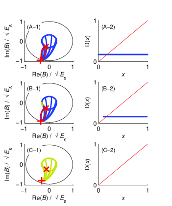
Figure 3: (color online) Resonator’s dynamics. Subplots A, B and C correspond to the three operating points A, B and C respectively which are marked in the inset of Fig. 2. In subplot (A) only a LC is locally stable, in subplot (B) intermittency between a LC and a SC steady state occurs, whereas only a SC steady state is locally stable in subplot (C). In panels (A-1), (B-1) and (C-1), which show the time evolution in $B$ plane, a plus sign labels $B_{\mathrm{s}}$ and a cross sign labels $B_{\mathrm{n}}$. These points are shown for reference and correspond to fixed points of the dynamics only when they exist in their respective domains, as defined in the text. Trajectories that return to the inner circle $\left|B\right|^{2}=E_{\mathrm{n}}$ are colored in blue (dark), and trajectories that end at $B_{\mathrm{s}}$ are colored in yellow (gray). Panels (A-2), (B-2) and (C-2) show the corresponding 1D maps.

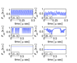
Figure 4: Numerical [panels (A-3), (B-3) and (C-3)] vs. experimental [panels (A-4), (B-4) and (C-4)] time traces for the three operating points A, B and C respectively.

The important features of the system’s dynamics can be captured by constructing a 1D map Strogatz (2000). Consider the case where $E_{\mathrm{n}}<E_{\mathrm{s}}$ and the amplitude $B$ lies initially on the circle $\left|B\right|^{2}=E_{\mathrm{n}}$, namely $B=\sqrt{E_{\mathrm{n}}}e^{2\pi ix}$ where $x\in[0,1]$. Furthermore, assume that initially the system is in the SC phase, namely, $T<T_{\mathrm{c}}$ and consequently $B$ is attracted towards the point $B_{\mathrm{s}}$. The 1D map $D\left(x\right)$ is obtained by tracking the time evolution of the system for the noiseless case ($c^{\mathrm{in}}=0$) until the next time it returns to the circle $\left|B\right|^{2}=E_{\mathrm{n}}$ to a point $B=\sqrt{E_{\mathrm{n}}}e^{2\pi iD\left(x\right)}$ where $D\left(x\right)\in[0,1]$. In the adiabatic limit this can be done using Eq. (1) only [without explicitly referring to Eq. (2)] since switching to the NC phase in this case occurs when the trajectory intersects with the circle $\left|B\right|^{2}=E_{\mathrm{s}}$. Note that in the aS zone of operation all points on the circle $\left|B\right|^{2}=E_{\mathrm{n}}$ return back to it after a finite time. However, this is not necessarily the case in the other stability zones. Therefore, we restrict the definition of the 1D map $D\left(x\right)$ only for points on the circle $\left|B\right|^{2}=E_{\mathrm{n}}$ that eventually return to it. Other points will have a trajectory that ends at a steady state (NC or SC).

Any fixed point of the 1D map, namely a point for which $D\left(x_{0}\right)=x_{0}$, represents a LC of the system. The LC is locally stable provided that $\left|\mathrm{d}D/\mathrm{d}x\right|_{x=x_{0}}<1$ Strogatz (2000). The region in the $\omega_{\mathrm{p}}$ - $P_{\mathrm{p}}$ plane in which a locally stable LC solution exists was determined using the parameters of our device and it is marked with dashed line in Fig. 2.

Figure 3 shows noiseless behvior of the resonator for the three operating points A, B and C, which lie near the border between the aS region and the MS(SC) one, and are marked in the inset of Fig. 2. Figure 4 shows a comparison of experimental data and numerical simulation for these operating points. The sample parameters used in the numerical simulations and are listed in the caption of Fig. 2, were determined using the same methods detailed in Ref. Segev et al. (2007c).

Subplot (A) shows the behavior at operating point A, which lies inside the aS zone. In panel (A-1) sample trajectories in $B$ plane are shown. The resultant 1D map, which is plotted in panel (A-2), has a single fixed point corresponding to a single locally stable LC. The time evolution seen in panel (A-3) was obtained by numerically integrating the coupled stochastic equations of motion (1) and (2). The trace is then compared to experimental data taken from the same working point [panel (A-4)].

At operating point B [see Fig 3 and 4 subplot (B)] coexistence of a LC and a SC steady state occurs. The LC corresponds to the locally stable fixed point of the 1D map seen in panel (B-2). On the other hand, all initial points on the circle $\left|B\right|^{2}=E_{\mathrm{n}}$ that never return to it evolve towards the SC steady state $B_{\mathrm{s}}$. Numerical time evolution and experimental data shows noise-induced transitions between the two metastable solutions [panels (B-3) and (B-4) respectively]. At operating point C [see Fig 3 and 4 subplot (C)] the LC has been annihilated by a discontinuity-induced bifurcation Bernardo et al. (2007) and consequently only steady state response is observed.

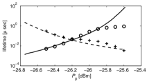
Figure 5: Experimental data of life time of LC (circles) and steady state (pluses) compared to numerical prediction (solid and dashed lines respectively). Mesurements above $-25.8\operatorname*{dBm}$ saturate to $1\mu\sec$ as this is the maximal mesuerment time.

To further study noise-induced transitions we fixed $\omega_{\mathrm{p}}$ and vary $P_{\mathrm{p}}$ starting from MS(SC) zone $P_{\mathrm{p}}=-26.7\operatorname*{dBm}$ to the aS zone $P_{\mathrm{p}}=-25.6\operatorname*{dBm}$ [vertical line in Fig. (2)], and took $1\mu\sec$ long time traces of $P_{\mathrm{ref}}$ [similar to those seen in Fig. 4 (A-4), (B-4) and (C-4)]. The average lifetime of both LC and SC steady state, namely, the average time the system is in one solution before making a transition to the other one, were determined from these traces. This data, compared to numerical simulation prediction is shown in Fig. 5.

In another experiment using a similar device we observe intermittency of two different LCs (see Fig. 6). Panel (A) shows spectrum analyzer measurement of the reflected power as a function of the pump power $P_{\mathrm{p}}$. Two distinct LCs having frequencies $f_{1}\simeq 60\operatorname{MHz}$ and $f_{2}\simeq 80\operatorname{MHz}$ are observed. For $P_{\mathrm{p}}<-33.5\operatorname*{dBm}$ only a LC at frequency $f_{1}$ is visible. In the range $-33.55\operatorname*{dBm}<P_{\mathrm{p}}<-33.35\operatorname*{dBm}$ both LCs are seen, whereas for high pump power $P_{\mathrm{p}}>-33.5\operatorname*{dBm}$ only a LC at frequency$\ f_{2}$ is seen. Panels (B) and (C), demonstrates the behavior in the intermediate region, where both LCs are observed in frequency and time domain respectively for $P_{\mathrm{p}}=-33.5\operatorname*{dBm}$ [marked by a dashed line in panel (A)].

In general, intermittency of two (or more) different LCs can be theoretically reproduced using our simple model. However, we were unable to numerically obtain this behavior without significantly varying some of the system’s experimental parameters. This discrepancy between experimental and theoretical results suggest that a further theoretical study is needed in order to develop a more realistic description of the system.

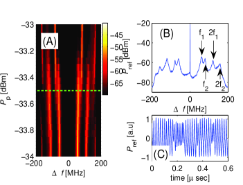
Figure 6: Experimental demonstration of intermittency between two LCs. Panel (A) shows the reflected power $P_{\mathrm{ref}}$ as a function of the offset frequency $\Delta f=(\omega-\omega_{p})/2\pi$ and the pump power $P_{\mathrm{p}}$. Panel (B) shows a cross section of panel (A) which is indicated by a dashed line. The frequencies $f_{1}$ and $f_{2}$ of the two LCs are marked. Panel (C) shows a time trace of the reflected power taken at the same value of $P_{\mathrm{p}}$. In this experiment $\omega_{p}/2\pi=6.61\operatorname{GHz}$

We thank Mike Cross, Mark Dykman, Oded Gottlieb and Ron Lifshitz for valuable discussions. This work was supported by the ISF, Deborah Foundation, Poznanski Foundation, RBNI and MAFAT.

References

- Movshovich et al. (1990) R. Movshovich, B. Yurke, P. G. Kaminsky, A. D. Smith, A. H. Silver, R. W. Simon, and M. V. Schneider, Phys. Rev. Lett. 65, 1419 (1990).
- Siddiqi et al. (2004) I. Siddiqi, R. Vijay, F. Pierre, C. M. Wilson, M. Metcalfe, C. Rigetti, L. Frunzio, and M. H. Devoret, Phys. Rev. Lett. 93, 207002 (2004).
- Castellanos-Beltran and Lehnert (2007) M. A. Castellanos-Beltran and K. W. Lehnert, Appl. Phys. Lett. 91, 083509 (2007).
- Tholen et al. (2007) E. A. Tholen, A. Ergul, E. M. Doherty, F. M. Weber, F. Gregis, and D. B. Haviland, Appl. Phys. Lett. 90, 253509 (2007).
- Lee et al. (2006) J. C. Lee, W. D. Oliver, K. K. Berggren, and T. P. Orlando, Arxiv: cond-mat/0609561 (2006).
- Segev et al. (2007a) E. Segev, B. Abdo, O. Shtempluck, and E. Buks, Phys. Lett. A 366, 160 (2007a).
- Segev et al. (2007b) E. Segev, B. Abdo, O. Shtempluck, and E. Buks, Euro. Phys. Lett. 78, 57002 (2007b).
- Segev et al. (2007c) E. Segev, B. Abdo, O. Shtempluck, and E. Buks, J. Phys.: Condens. Matter 19, 096206 (2007c).
- Berge et al. (1984) P. Berge, Y. Pomeau, and C. Vidal, Order Within Chaos (Wiley, New York, 1984).
- Ecke and Haucke (1989) R. Ecke and H. Haucke, Journal of Statistical Physics 54, 1153 (1989).
- Franck et al. (1999) C. Franck, T. Klinger, and A. Piel, Physics Letters A 259, 152 (1999).
- Stone and Holmes (1989) E. Stone and P. Holmes, Physica D 37, 20 (1989).
- Pedaci et al. (2005) F. Pedaci, M. Giudici, J. R. Tredicce, and G. Giacomelli, Phys. Rev. E 71, 036125 (2005).
- Kuno et al. (2000) M. Kuno, D. P. Fromm, H. F. Hamann, A. Gallagher, and D. J. Nesbitt, J. Chem. Phys. 112, 3117 (2000).
- Longtin et al. (1991) A. Longtin, A. Bulsara, and F. Moss, Phys. Rev. Lett. 67, 656 (1991).
- Chialvo and Jalife (1990) Chialvo and J. Jalife, Cardiac Electrophysiology: From Cell to Bedside (Saunders, 1990), chap. 24, pp. 201–214.
- Eckmann et al. (1981) J. Eckmann, L. Thomas, and P. Wittwer, J. Phys. A: Math Gen. 14, 3153 (1981).
- Haucke et al. (1984) H. Haucke, R. E. Ecke, Y. Maeno, and J. C. Wheatley, Phys. Rev. Lett. 53, 2090 (1984).
- Sommerer et al. (1991a) J. Sommerer, E. Ott, and C. Grebogi, Phys. Rev. A 43, 1754 (1991a).
- Sommerer et al. (1991b) J. C. Sommerer, W. L. Ditto, C. Grebogi, E. Ott, and M. L. Spano, Phys. Rev. Lett. 66, 1947 (1991b).
- Bernardo et al. (2007) M. D. Bernardo, C. Budd, A. Champneys, and P. Kowalczyk, Piecewise-Smooth Dynamical Systems: Theory and Applications (Springer-Verlag, 2007), applied Mathematics series no. 163.
- Segev et al. (2006) E. Segev, B. Abdo, O. Shtempluck, and E. Buks, IEEE Trans. Appl. Supercond. 16, 1943 (2006).
- Chang et al. (1987) K. Chang, S. Martin, F. Wang, and J. L. Klein, IEEE Trans. Microwave Theory Tech. MTT-35, 1733 (1987).
- Saeedkia et al. (2005) D. Saeedkia, A. H. Majedi, S. Safavi-Naeini, and R. R. Mansour, IEEE Microwave Wireless Compon. Lett. 15, 510 (2005).
- Strogatz (2000) S. Strogatz, Nonlinear Dynamics and Chaos (Perseus Books Group, 2000).