Comparison of statistical treatments for the equation of state for
core-collapse supernovae

Abstract

Neutrinos emitted during the collapse, bounce and subsequent explosion provide information about supernova dynamics. The neutrino spectra are determined by weak interactions with nuclei and nucleons in the inner regions of the star, and thus the neutrino spectra are determined by the composition of matter. The composition of stellar matter at temperature ranging from $T=1-3$ MeV and densities ranging from $10^{-5}$ to $0.1$ times the saturation density is explored. We examine the single-nucleus approximation commonly used in describing dense matter in supernova simulations and show that, while the approximation is accurate for predicting the energy and pressure at most densities, it fails to predict the composition accurately. We find that as the temperature and density increase, the single nucleus approximation systematically overpredicts the mass number of nuclei that are actually present and underestimates the contribution from lighter nuclei which are present in significant amounts.

1. Introduction

Stars with masses larger than about 10 M_⊙ end their lives in core-collapse supernovae. The initial collapse is initiated by the disappearance of the pressure support driven by (i) dissociation of nuclei and (ii) electron capture on nuclei which make matter increasingly neutron rich. The electron captures emit neutrinos, which initially escape, but are later trapped by the increasing density in the core. The collapse is halted by the strong repulsion from high density matter and the core “bounces,” driving an outward shock wave. The standard view is that this shock loses energy through continuing dissociation of nuclei and neutrinos from the core finally restore energy to the shock driving an explosion.

The evolution of the supernova is determined by the equation of state (EOS) and composition of matter at densities up to the nuclear saturation density, $\rho_{0}\sim 2.7\times 10^{14}~{}\mathrm{g/cm}^{3}$ and at temperatures between 1 and 3 MeV. The collapse is driven by the tendency of matter to have a low entropy per baryon (Bethe et al., 1979), the extent of electron captures during collapse is determined by the composition (Hix et al., 2003), and the neutrino spectrum (Sumiyoshi et al., 2005) is determined by the nature of matter at the “neutrinosphere”, the surface of the last neutrino scattering, which is typically at $10^{11}$ g/cm³.

At densities below $\rho\sim 8\times 10^{13}~{}\mathrm{g/cm}^{3}$, most matter resides in nuclei with $A\geq 10$ arranged in a Coulomb lattice, surrounded by a nucleon gas and embedded in a degenerate electron gas. Masses of isolated nuclei in coexistence with the gas may exceed those of stable nuclei but are limited to $A<1000$ by the interplay of the Coulomb and symmetry contributions to their binding energies. Both nucleons and nuclei together compose a nuclear (Fermi) liquid-gas phase mixture, whose Equation of State (EOS) contributes significantly to the EOS for supernova simulations.

A principal approach to computing the EOS for supernovae used in the past three decades has been the “Single-Nucleus Approximation” (SNA) where low-temperature matter is assumed to be composed of neutrons, protons, alpha particles, and a single, representative, heavy nucleus (Lattimer et al., 1985; Lattimer & Swesty, 1991; Shen et al., 1998). The nuclei vaporize at temperatures that depend sensitively on density. Burrows & Lattimer (1984) have found that the SNA can accurately predict thermodynamic functions for the matter, and microscopic calculations for the nuclear matter EOS have been performed in this approximation for densities ranging from 0 to saturation density (Lattimer et al., 1985; Lattimer & Swesty, 1991; Shen et al., 1998). However, recent studies suggest that the SNA may be insufficient to completely describe the dynamics of core-collapse supernovae. In particular, Hix et al. (2003) find that calculating electron captures on a distribution of nuclei in nuclear statistical equilibrium, in place of a single representative nucleus, increased the potential for an explosion. Also, Arcones et al. (2008) find that the presence of light nuclei is important for describing the neutrino spectra in the early post-explosion phase.

A more realistic description of supernovae EOS would model the composition of matter by an ensemble of nuclei in near nuclear statistical equilibrium. In this work, we refer to this approach as the “Grand Canonical Approximation” (GCA). The GCA permits investigation of the shapes and widths of the nuclear mass and charge distributions and the population of nuclear excited states. In situations where the Wigner-Seitz approximation for a unit cell is valid and the widths of the heavy nuclear distributions can be neglected, GCA and SNA models should make similar predictions. In a recent paper Botvina & Mishustin (2005) report on GCA calculations for supernovae and suggest that differences between their GCA and previous SNA calculations should be important. However, they did not directly compare SNA and GCA approximations to quantify the differences.

To address this question, we adopt a GCA model that is formally equivalent to that of Botvina & Mishustin (2005), and construct an analagous SNA model for comparisons to the GCA model. This corresponding SNA model employs the same mass formula and level densities that are used in a corresponding GCA model. We compare predictions of the GCA model and its companion SNA model for two different mass formulae, which differ by their treatment of the nuclear surface symmetry energy. Then, we construct another SNA model (ISNA) which is more similar to the modern tabulated EOS constructed in Lattimer & Swesty (1991) and is frequently employed in supernovae simulations. The ISNA model includes interactions and the quantum statistics of the nucleons in the gas, a more complete description of the Coulomb energy, surface energy term which vanishes in the small proton number limit, a critical temperature which depends on the electron fraction, and effects associated with the presence of a neutron skin for nuclei with $N>Z$.

From comparisons between the GCA and SNA models, we find that the traditional SNA approach succeeds at most densities in describing the basic properties of the equation of state, but that it fails in describing the composition. We find that the differences between the predictions of GCA models and SNA models exceeds the differences between the predictions of the various SNA models. More specifically, we find that average quantities, such as the mass fractions for neutrons, $\alpha$ particles and heavy nuclei, energy/baryon, and entropy, are similar at $\rho\leq 0.01$ and $Y_{e}=0.4$ in the GCA and SNA approaches. The agreement is slightly worse for $Y_{e}=0.2$, and the agreement between GCA and SNA deteriorates even more for calculations that neglect the surface symmetry energy.

We find generally that the SNA and ISNA models agree quite well over most of the densities and temperatures considered; the largest differences are a few tenths of an MeV in the energy per baryon at higher densities and comparable differences in the entropy. The SNA and ISNA calculations, however, neglect completely the considerable widths of the mass and charge distributions predicted by the GCA calculations. At higher temperatures and densities, the SNA calculations systematically over-predict the size of the representative nucleus, and fail to treat the light nuclei that become more abundant in some regimes of density and temperature. These differences can have an impact on the electron capture and weak interaction rates that prevail in a supernova.

In the following, we begin our comparisons by adopting identical formula for the masses, level densities, and electron screening approximations for pairs of GCA and SNA calculations. We perform this comparison for two liquid drop models, LDM1, which has a surface symmetry energy term, and LDM2, which does not. Section 2 describes these model assumptions. As these two calculations neglect the interactions and quantum statistics of particles in the gas, the ISNA model that contains these effects is described in Section 2 as well. Section 3 describes and compares results obtained for the various GCA and SNA models. Section 4 summarizes this work and provides an outlook for future studies.

2. The models

Sections 2.1-2.3 describe the SNA and GCA models without the inclusion of the interactions and quantum statistics of particles in the gas. These two calculations can be compared to isolate the differences between the SNA and CGA models. Section 2.4 describes an improved SNA model (the ISNA model) that includes the interactions and quantum statistics of particles in the gas. This model allows tests of the relative importance of some simplifying assumptions used in the models described in Sections 2.1-2.3.

2.1. Ground State Properties of Nuclei

The binding energies of nuclei strongly influence the charge and mass distributions of nuclei within hot extended nuclear systems (Souza et al., 2003; Tan et al., 2003). In this work we use a form for the liquid drop mass formula from (Preston & Bhaduri, 1975):

$$B_{A,Z}=C_{v}A-C_{s}A^{2/3}-C_{c}\frac{Z^{2}}{A^{1/3}}+\delta_{A,Z}A^{-1/2}+C_{d}\frac{Z^{2}}{A}\;,$$ (1)

where $A$ and $Z$ denote, respectively, the mass and atomic numbers,

$$C_{i}=a_{i}\left[1-k_{i}\left(\frac{A-2Z}{A}\right)^{2}\right]\;,$$ (2)

and $i=v,s$ corresponds to volume and surface, respectively. In Souza et al. (2003), its parameters have been fitted to the available experimental data (Audi & Wapstra, 1995). The corresponding values are listed in Table 1, and are labeled LDM1 (Liquid Drop Model). For completeness, the pairing term is also included in the expression above, although it is neglected in the calculations presented in this paper. It reads:

$$\delta_{A,Z}=\left\{\begin{array}[]{rl}+C_{p},&N\,{\rm and}\,Z\,{\rm even}\\ 0,&A\,\,{\rm odd}\\ -C_{p},&N\,{\rm and}\,Z\,{\rm odd}\\ \end{array}\right.\;,$$ (3)

where $N=A-Z$ stands for the number of neutrons. Besides the standard terms, this parametrization includes a correction to the Coulomb energy due to the diffuseness of the surface, $C_{d}Z^{2}/A$, as well as a surface contribution to the symmetry energy. Both corrections are usually neglected in simple parametrizations. While the latter contribution is most important for light nuclei, it also influences the masses of very heavy nuclei, as discussed below.

Table 1Parameters of the liquid drop mass formulas used in this work. All the values are given in MeV.

Label	$a_{v}$	$a_{s}$	$C_{c}$	$C_{d}$	$C_{p}$	$a_{v}k_{v}$	$a_{s}k_{s}$
LDM1	15.6658	18.9952	0.72053	1.74859	10.857	27.7976	33.7053
LDM2	15.2692	16.038	0.68698	0.0	11.277	22.3918	0.0
	$n_{s}$	$n_{d}$	${\cal C}$	$\zeta$	$\sigma$	$b$
LDM3	0.1764	-0.2832	0.8990	0.9467	1.179	9.130

The accuracy of this formula can be inferred from Figure 1, which shows the difference $\Delta B$ between the predictions of equation (1) and the empirical (measured) values. It is important to stress that $\Delta B$ corresponds to the difference between the total binding energies, i.e., it is not divided by the mass number. Since the above formula has no corrections associated with shell effects, pronounced discrepancies are observed near closed shells. Shell effects for nuclei with $A>5$ are neglected since they do not strongly modify the qualitative shape of the nuclear distributions which we calculate.

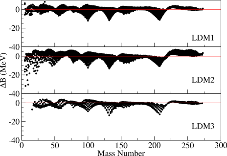
Figure 1.— Difference between the total binding energy predicted by the mass formula and the empirical values. For details, see the text.

In order to investigate the influence of the Coulomb diffuseness correction and the surface symmetry energy, we have refitted the data while keeping the parameters $C_{d}$ and $k_{S}$ equal to zero. In this limit, this mass formula has no surface symmetry energy or diffuseness correction to the Coulomb interaction, which makes it have the same form that is used in many statistical calculations (Botvina & Mishustin, 2005, 2004; Aguiar et al., 2006; Bhattacharyya & Mekjian, 1999; Bondorf et al., 1995). The best fit parameters are listed in Table 1 and labeled LDM2. The corresponding deviations $\Delta B$ from the empirical values are shown in the middle panel of Figure 1. One can clearly see tendencies for LDM2 to over predict the empirical values for heavy masses and even stronger tendencies to under predict the empirical values for light masses.

To aid in the discussion we define the nuclear symmetry energy, $B_{\rm sym}$:

$$B_{\rm sym} = -\left(a_{v}k_{v}-\frac{a_{s}k_{s}}{A^{1/3}}\right)\frac{(A-2Z)^{2}}{A}$$ (4)

$$\equiv -a_{\rm sym}\frac{(A-2Z)^{2}}{A}\;(\mathrm{for}~{}\mathrm{LDM2}).$$

The second line shows the simplification that occurs by setting $k_{s}=0$ in the LMD2 parametrization.

The difference between the LDM1 and LDM2 reflects the reduction of the symmetry energy in the nuclear surface and in the effective symmetry energy coefficient $a_{\rm sym}$ in the LMD1 parametrization, which causes its masses to increase as a function of $A$, better following the trends of the measured masses. In the simpler LDM2 parametrization, this coefficient is constant, which does not accurately follow the experimental trends and leads to the systematic deviations in both the light and heavy mass regions displayed in the figure. We have checked that the influence of the $C_{d}$ coefficient does not account for the increase in $\Delta B$ observed in the heavy mass region.

Experimental values are used for the very light nuclei ($A<5$), whenever known, since both parameter sets give a very poor description of the binding energies of light nuclei. This procedure is not adopted for heavier nuclei as one has to consider nuclei far from the known mass region. In this case, a careful extrapolation scheme should be devised so as not to introduce spurious effects in the calculated yields for mass regions in which no experimental information is available (Souza et al., 2003; Tan et al., 2003). Since the major thrust of this paper concerns the comparison of two approximations for calculating equilibrium distributions of nuclei, the use of a mass formula for all nuclei with $A>4$ is sufficient and will ensure a smooth behavior for the predicted yields throughout the mass range considered below.

A similar procedure is also adopted for the spin degeneracy factors of nuclei. Empirical values are used only for $A<5$. For heavier nuclei, we set the spin degeneracy factors to unity (vanishing nuclear spin). This approximation is not that important because errors introduced by neglecting ground state spin degeneracies are much smaller than the uncertainties in the nuclear level densities at finite temperatures. These level densities are described below.

2.2. The Grand Canonical Approximation (GCA)

For a system composed of $\{k_{1},k_{2},\cdots,k_{M}\}$ different species in thermal equilibrium at temperature $T$, the grand-partition function is given by

$$Z_{G}= \sum_{k_{1}=0}^{\infty}\cdots\sum_{k_{M}=0}^{\infty}Z_{C}(T,V,k_{1},k_{2},\cdots,k_{M})$$ (5)

$$e^{\beta(\mu_{1}k_{1}+\mu_{2}k_{2}+\cdots+\mu_{M}k_{M})}\;,$$

where $\beta\equiv 1/T$, and the canonical partition function $Z_{C}$ is given by

$$Z_{C}= \frac{\left[g_{1}V_{f}A_{1}^{3/2}/\lambda_{T}^{3}\right]^{k_{1}}}{k_{1}!}\cdots\frac{\left[g_{M}V_{f}A_{M}^{3/2}/\lambda_{T}^{3}\right]^{k_{M}}}{k_{M}!}$$ (6)

$$\times e^{-\beta F(T,V,k_{1},\cdots,k_{M})}\;.$$

In the above expression, $\lambda_{T}=\sqrt{2\pi\hbar^{2}/mT}$, we approximate the nucleus translational effective mass by $m_{A,Z}=Am$ following Tan et al. (2003). We further approximate $m$ by the free nucleon mass $m=939$ MeV/$c^{2}$. The function $F(T,V,k_{1},\cdots,k_{M})$ denotes the Helmholtz free energy of the system, excluding contributions associated with the translational motion, and $g_{i}$ denotes the spin degeneracy factor. The free volume $V_{f}$ takes finite size effects into account and is calculated as in Botvina & Mishustin (2004), i.e., $\Omega\equiv V_{f}/V=1-\rho_{B}/\rho_{0}$, where $V$ is the total volume, $\rho_{B}$ denotes the baryon density, and $\rho_{0}$ represents normal (saturation) nuclear density. If $F(T,V,k_{1},\cdots,k_{M})$ can be written as

$$F=k_{1}f_{1}(T,V)+k_{2}f_{2}(T,V)+\cdots+k_{M}f_{M}(T,V)\;,$$ (7)

the canonical partition function becomes

$$Z_{C}(T,V,k_{1},\cdots,k_{M})=\prod_{i=1}^{M}\frac{\left[g_{i}V_{f}A_{i}^{3/2}/\lambda_{T}^{3}\right]^{k_{i}}}{k_{i}!}e^{-\beta f_{i}k_{i}}\;,$$ (8)

which leads to

$$Z_{G}(T,V,\{\mu_{i}\})=\prod_{i=1}^{M}e^{q_{i}}\;,$$ (9)

where

$$q_{i}=\frac{g_{i}V_{f}A_{i}^{3/2}}{\lambda_{T}^{3}}e^{\beta(\mu_{i}-f_{i})}\;.$$ (10)

In this case, the average number of nuclei of species $i$ in the volume $V$, $Y_{i}$, can be easily evaluated

$$Y_{i}=\frac{1}{Z_{G}}\sum_{k_{1}=0}^{\infty}\frac{q_{i}^{k_{1}}}{k_{1}!}\cdots\sum_{k_{i}=0}^{\infty}k_{i}\frac{q_{i}^{k_{i}}}{k_{i}!}\cdots\sum_{k_{M}=0}^{\infty}\frac{q_{M}^{k_{M}}}{k_{M}!}=q_{i}\;.$$ (11)

By assuming chemical equilibrium, the chemical potentials may be written as

$$\mu_{A,Z}=\mu_{B}A+\mu_{Q}Z,$$ (12)

so that the number density of a given species $(A,Z)$ becomes

$$n_{A,Z}=\frac{q_{A,Z}}{V}=\frac{g_{i}\Omega A^{3/2}}{\lambda_{T}^{3}}e^{(\mu_{B}A+\mu_{Q}Z-f_{A,Z})/T}\;.$$ (13)

Thus, $\mu_{B}$ and $\mu_{Q}$ are determined upon fixing the average number of baryons and by imposing charge neutrality, respectively:

$$n_{B}=\sum_{A,Z}A\,n_{A,Z}$$ (14)

$$n_{e}=\sum_{A,Z}Z\,n_{A,Z}\;,$$ (15)

where $n_{e}$ denotes the electron density. As in Botvina & Mishustin (2004), the sums include all nuclei with $Z\leq A$. We have checked that, for the temperatures and densities considered below, $A=1000$ is a safe upper cut in the sums above. We impose that the relative errors in equations (14-15) are smaller than $10^{-7}$.

In order to determine the chemical potentials, and subsequently, other relevant thermodynamical quantities, the Helmholtz free energy $f_{A,Z}$ must be specified. We include contributions to the internal excitation of nuclei associated with surface and bulk, besides the binding energy of the nuclei and the Coulomb interaction among the particles:

$$f_{A,Z} = \beta(T)A^{2/3}-\frac{T^{2}}{\epsilon_{0}}A-B_{A,Z}$$ (16)

$$+ C_{C}\frac{Z^{2}}{A^{1/3}}\left[-\frac{3}{2}\left(\frac{n_{B}}{n_{0}}\right)^{1/3}+\frac{1}{2}\left(\frac{n_{B}}{n_{0}}\right)\right]\;,$$

where

$$\beta(T)=\beta_{0}\left[\left(\frac{T_{c}^{2}-T^{2}}{T_{c}^{2}+T^{2}}\right)^{5/4}-1\right]\;.$$ (17)

The values of the parameters $\beta_{0}=18.0$ MeV, $T_{c}=18.0$ MeV, and $\epsilon_{0}=16.0$ MeV correspond to those usually adopted in statistical calculations (Aguiar et al., 2006; Botvina & Mishustin, 2004; Souza et al., 2003; Tan et al., 2003; Bondorf et al., 1995). The Coulomb energy, in the last term in equation (16), is calculated through the Wigner-Seitz approximation (Wigner & Seitz, 1934). It should be noted that equation (16) differs from the usual expressions employed in statistical models because it takes into account the presence of the electron gas surrounding the nuclei (Baym et al., 1971). In this respect, an important comment is in order. In principle, the baryon density in equation (16) should be the average particle density in the Wigner-Seitz cell (Baym et al., 1971). However, if this is done, the Helmholtz free energy cannot be cast in the form of equation (7) and, then, the simple formulae above would no longer be valid. Thus, as in Botvina & Mishustin (2004), we approximate the average density by $n_{B}$ in order to keep the simple relations above. Since we want to maintain the GCA and the SNA close as possible, we adopt this approximation in SNA model as well.

Finally, nuclei with $A<4$ are treated as point particles, with no internal degrees of freedom. Therefore, the temperature dependent terms in equation (16) are set to zero for those nuclei.

2.3. The Single Nucleus Approximation (SNA)

Since the determination of the chemical potentials above and the subsequent computation of the relevant thermodynamical quantities is too time consuming to be used in many practical astrophysical calculations, the GCA has been simplified (Epstein & Arnett, 1975; Burrows & Lattimer, 1984; Lattimer et al., 1985; Lattimer & Swesty, 1991). More specifically, instead of considering all possible species, only a few types are allowed: neutrons, protons, alpha particles and a single species of heavy nucleus. The latter should, to some extent, represent the nucleus distribution at the heavy mass region. The other three nuclei are intended to consider the main contribution to the nucleus distribution in the light mass region.

The constraints associated with baryon number and charge neutrality simplify to

$$n_{B}=n_{n}+n_{p}+4n_{\alpha}+A_{h}n_{h}$$ (18)

and

$$n_{e}=n_{p}+2n_{\alpha}+Z_{h}n_{h}\;,$$ (19)

where $n_{n}$, $n_{p}$, $n_{\alpha}$, and $n_{h}$ respectively denote the number density of neutrons, protons, alpha particles, and the heavy nucleus of mass and atomic numbers $A_{h}$ and $Z_{h}$. In this way, the most probable configuration is found by minimizing the total free energy of the system ${\cal F}$, subject to the above constraints

$$\frac{\partial}{\partial x_{i}}\{{\cal F} - V\lambda_{1}\left[n_{B}-n_{n}-n_{p}-4n_{\alpha}-A_{h}n_{h}\right]$$ (20)

$$- V\lambda_{2}\left[n_{e}-n_{p}-2n_{\alpha}-Z_{h}n_{h}\right]\}=0\;.$$

In this expression, $\lambda_{i}$ stands for the Lagrange-multipliers and $x_{i}$ denotes $A_{h}$, $Z_{h}$, $n_{n}$, $n_{p}$, $n_{\alpha}$, and $n_{h}$. The total Helmholtz free energy possesses the same ingredients used in the GCA:

$${\cal F} = V[(f_{n}+f_{n}^{\rm trans})n_{n}+(f_{p}+f_{p}^{\rm trans})n_{p}$$ (21)

$$+ (f_{\alpha}+f_{\alpha}^{trans})n_{\alpha}+(f_{h}+f_{h}^{\rm trans})n_{h}]\;.$$

The contribution due to the translational motion is given by

$$f_{i}^{\rm trans}=-T\left[\log\left(\frac{g_{i}V_{f}}{\lambda_{T}^{3}}A^{3/2}\right)-\frac{\log(k_{i}!)}{k_{i}}\right]$$ (22)

and, for large values of $k_{i}$, one may write

$$f_{i}^{\rm trans}=-T\left[\log\left(\frac{g_{i}\Omega}{\lambda_{T}^{3}n_{i}}A^{3/2}\right)+1\right]\;,$$ (23)

since $\log(k_{i}!)\approx k_{i}\log(k_{i})-k_{i}$.

The derivatives associated with $n_{n}$ and $n_{p}$ allow one to easily eliminate the Lagrange multipliers:

$$\lambda_{1}=T\log\left(\frac{g_{n}\Omega}{\lambda_{T}^{3}n_{n}}\right)$$ (24)

$$\lambda_{2}=T\log\left(\frac{n_{n}}{n_{p}}\right)-C_{c}\left[-\frac{3}{2}\left(\frac{n_{B}}{n_{0}}\right)^{1/3}+\frac{1}{2}\left(\frac{n_{B}}{n_{0}}\right)\right]\;.$$ (25)

The remaining derivatives, with respect to $A_{h}$, $Z_{h}$, $n_{\alpha}$, and $n_{h}$, lead to non-linear equations, which must be solved numerically. Due to the logarithmic factors entering in the formulae, it is convenient to use

$$n_{i}=\frac{g_{i}\Omega}{\lambda_{T}^{3}}A_{i}^{3/2}e^{-(f_{i}-\mu_{i})/T}\;,$$ (26)

so that the equations are solved for the chemical potentials of each species. We require the same precision on the constraints (18-19) as in the grand canonical calculations.

2.4. A Single Nucleus Approximation with Interactions (ISNA)

This improved single nucleus model (ISNA) uses the mass formula from Steiner (2008), adapted slightly to include finite temperature, alpha particles, and the effects of the neutron skin. In this model, the binding energy of a nucleus at temperature $T$, with proton number $Z$ and mass number $A$, in the presence of an external proton gas of density $n_{p,\mathrm{out}}$, is given by

$$B(Z,A,n_{n},n_{p},n_{p,\mathrm{out}},T)=B_{\mathrm{bulk}}(n_{n},n_{p},T)$$

$$+\sigma{\cal B}(n_{n},n_{p},T)\left(\frac{36\pi A^{2}}{n^{2}}\right)^{1/3}$$

$$+{\cal C}~{}\varepsilon_{\mathrm{Coulomb}}(Z,A,n_{p,\mathrm{out}})/(An).$$ (27)

Here, $n_{n}$, $n_{p}$ and $n=n_{n}+n_{p}$ denote the average internal neutron, proton and baryon number densities, respectively.

The binding free energy of bulk matter, $B_{\mathrm{bulk}}$ is given by

$$B_{\mathrm{bulk}} = \frac{A-N_{\mathrm{skin}}}{n}\left[\varepsilon(n_{n},n_{p},T)-n_{n}m_{n}-n_{p}m_{p}\right.$$ (28)

$$\left.-Ts(n_{n},n_{p},T)\right]+\frac{N_{\mathrm{skin}}}{n}\left[\varepsilon(n_{n},0,T)-n_{n}m_{n}\right.$$

$$\left.-Ts(n_{n},0,T)\right]$$

where $m_{n}$ and $m_{p}$ are the neutron and proton masses, $\varepsilon(n_{n},n_{p},T)$ is the energy density of homogeneous matter evaluated at the given neutron and proton density and temperature, and $s(n_{n},n_{p},T)$ is the entropy density. The energy density of homogeneous matter is described using the Akmal, Pandharipande, and Ravenhall EOS (Akmal et al., 1998, APR). Finite temperature corrections to the APR EOS are computed assuming that there are no finite temperature corrections to the potential energy contributions similar to the approach used in Prakash et al. (1997). The part proportional to $N_{\mathrm{skin}}$ is a correction to the bulk energy density for the neutron skin.

The average baryon density in equation (28) is determined from

$$n=n_{n}+n_{p}=n_{s}+n_{d}I^{2}$$ (29)

where $I=1-2Z/A$. The parameter $n_{s}$ is analogous to the saturation density of nuclear matter and is expected to be near 0.16 fm^-3. The parameter $n_{d}$ (which is typically negative) subsumes the decrease in the saturation density with the isospin asymmetry.

The individual average neutron and proton number densities are given by

$$n_{n} = n(1+\delta)/2$$

$$n_{p} = n(1-\delta)/2$$ (30)

and the density asymmetry $\delta=1-2n_{p}/(n_{n}+n_{p})$ is given by $\delta=\zeta I$ where $\zeta$ is a constant parameter determined by the fit to the experimental nuclear masses.

The parameter $N_{\mathrm{skin}}$ is chosen so that

$$A-N_{\mathrm{skin}}=\frac{4\pi}{3}R_{p}^{3}(n_{n}+n_{p}).$$ (31)

The neutron and proton radii, $R_{n}$ and $R_{p}$ are fixed by

$$A-Z = \frac{4\pi}{3}R_{n}^{3}n_{n}$$

$$Z = \frac{4\pi}{3}R_{p}^{3}n_{p}.$$ (32)

In summary, for the bulk part of the nuclear mass formula, using $Z$ and $A$ one can compute the average neutron and proton densities using the relations above, and the radii from equations (32), then compute $N_{\mathrm{skin}}$ from equation (31), and use the equation of state for homogeneous matter to compute the bulk part in equation (28) above. Note that the symmetry energy contribution to the nuclear mass is automatically counted above as part of the bulk contribution.

The surface energy density as a function of the “surface tension”, $\sigma$ is

$$\varepsilon_{\mathrm{surface}}=\frac{3\sigma}{R}$$ (33)

For the mass formula, we need the surface energy per baryon, which for $T=0$ and $I=0$ is given by

$$B(T=0,I=0)_{\mathrm{surface}}/A=\frac{d\sigma}{nR}.$$ (34)

Where the radius, $R$ is determined from

$$\frac{4\pi R^{3}}{3}n=A$$ (35)

so that

$$B(T=0,I=0)_{\mathrm{surface}}/A=\frac{3\sigma}{n}\left(\frac{4\pi n}{3A}\right)^{1/3}$$ (36)

In general, the surface energy should be modified to ensure that the surface energy vanishes in the limit $\delta\rightarrow 1$ as it must. To address this issue, we follow Lattimer et al. (1985) and approximate ${\cal B}(n_{n},n_{p},T)$ by:

$${\cal B}(n_{n},n_{p},T) = \eta(n_{n},n_{p},T)\frac{16+b}{\left[1/x^{3}+b+1/(1-x)^{3}\right]}$$ (37)

$$\times B(T=0,I=0)_{\mathrm{surface}},$$

where $x=n_{p}/n$ and $b$ is a free parameter.

For $T>0$, one must consider the reduction in the surface tension of the nucleus due to the interactions with the surrounding gas. For the finite temperature correction, we follow (Lattimer et al., 1985) and approximate $\eta(n_{n},n_{p},T)$ by:

$$\eta(n_{n},n_{p},T)=\left[\frac{\left(1-T^{2}/T_{C}^{2}\right)}{\left(1+aT^{2}/T_{C}^{2}\right)}\right]^{5/4}.$$ (38)

This expression is essentially identical to the SNA model except for the presence of the factor $a=0.935-5.1(0.5-x)^{2}-1.1(0.5-x)^{4}$, which is obtained from a fit to the results of Ravenhall et al. (1972) that allows extrapolations to neutron rich systems. The critical temperature is also isospin dependent. Following Lattimer et al. (1985), we extrapolate $T_{C}$ to neutron rich matter using $T_{C}=T_{C}(x=1/2)\sqrt{1-3.313(0.5-x)^{2}-7.362(0.5-x)^{4}}$. We also take $T_{c}(x=1/2)=20.085$ MeV as was done by Lattimer et al. (1985).

The Coulomb energy density (Ravenhall et al., 1983) is

$$\varepsilon_{\mathrm{Coulomb}} = \frac{2}{5}\pi\left(n_{p}-n_{p,\mathrm{out}}\right)^{2}e^{2}R_{p}^{2}$$ (39)

$$\times\left[2-\chi_{p}^{1/3}+\chi_{p}\right]$$

where $e^{2}$ is the usual Coulomb coupling $\sim\hbar c/137$ and $\chi_{p}=R_{p}^{3}/R_{n}^{3}$ is the volume fraction of matter occupied by the proton sphere. The Coulomb contribution is multiplied in equation (27) by a final parameter, ${\cal C}$, which takes into account the fact that the proton density distribution has its own surface. The parameter values are given in Table 1 and labeled LDM3.

In order to determine the composition and properties of matter in the supernova, we minimize the free energy at a fixed density as a function of the proton number and atomic number of nuclei, and the number density of dripped neutrons, $n_{n,drip}$. The free energy of this matter is given by

$$f(Z,A,n_{n,\mathrm{out}},n_{p,\mathrm{out}},n_{\alpha,\mathrm{out}},T)=$$

$$nB(Z,A,n_{n,\mathrm{out}},n_{p,\mathrm{out}},T)/A$$

$$+(1-\chi)\left[{f}(n_{n,\mathrm{out}},n_{p,\mathrm{out}},T)\right.$$

$$+\left.{f}(n_{\alpha,\mathrm{out}},T)\right]+{f}_{\mathrm{Classical}}(n_{\mathrm{Nuclei}},T)+{f}_{\mathrm{el}}(n_{e},T)$$ (40)

where $n_{\mathrm{Nuclei}}=\chi n/A$, $\chi$ is the volume fraction of matter occupied by nuclei, and ${f}_{\mathrm{Classical}}(n_{\mathrm{Nuclei}},T)$ is the classical free energy from the ideal gas of nuclei, and ${f}_{\mathrm{el}}(n_{e})$ is the free energy of the electrons. For the purposes of comparisons with the SNA and GCA models, we do not include the free energy of the electrons in the ISNA calculations presented in this paper. The free energy of the dripped nucleons, ${f}(n_{n,\mathrm{out}},n_{p,\mathrm{out}},T)$, is computed with the APR EOS in the same way as the bulk contribution to the nuclear mass formula referred to above.

The constraints of baryon and charge conservation are implemented with

$$n_{B} = \chi n_{n}+\chi_{p}n_{p}+\left(1-\chi\right)n_{n,\mathrm{out}}+\left(1-\chi_{p}\right)n_{p,\mathrm{out}}$$

$$+4\left(1-\chi\right)n_{\alpha}$$

$$Y_{e}n_{B} = \chi_{p}n_{p}+\left(1-\chi_{p}\right)n_{p,\mathrm{out}}+2\left(1-\chi\right)n_{\alpha}$$ (41)

One of the two constraints is used to fix $\chi$, and the other can be used to constrain one of the parameters to the free energy, e.g. $n_{p,\mathrm{out}}$.

3. Results and Discussion

We utilize the models described above to compute the composition and thermodynamic functions for matter for the densities $10^{-5}<n_{B}/n_{0}<10^{-1}$, temperatures $1~{}\mathrm{MeV}<T<3~{}\mathrm{MeV}$, and electron fractions, $0.2<Y_{e}<0.4$ relevant for core-collapse supernovae, see e.g. Janka et al. (2007).

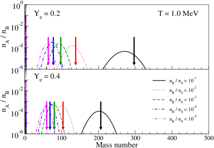
Figure 2.— Isobar number density for different values of $n_{B}$ at $T=1.0$ MeV, using the LDM1 mass model. The lines represent the results obtained with the GCA, whereas the arrows point to the values of $A_{h}$ predicted by SNA at the same values of $n_{B}$ used in the GCA. The baryon densities associated with the arrows increase from left to right.

The isobar number density

$$n_{A}=\sum_{Z}n_{A,Z}$$ (42)

is calculated through equation (13) using the LDM1, and the results are displayed in Figure 2 for different baryon densities at $T=1.0$ MeV and for two representative values of the electron fraction used throughout this work. The lines correspond to the distribution predicted by the GCA, whereas the arrows indicate the value of $A_{h}$ in SNA. The results reveal that $A_{h}$ is systematically larger than the mass number $A_{\rm max}$ at which the maximum of the isobar number density occurs, in the heavy mass region. This may be explained by noticing that heavy nuclei, many of them heavier than $A_{\rm max}$, contribute significantly to the sums in equations (14) and (15) due to the smooth behavior of $n_{A,Z}$. These contributions also include lighter nuclei such as the hydrogen isotopes (d,t), helium isotopes (³He, ⁶He) and intermediate mass nuclei with $3\leq Z\leq 20$. These other contributions, combined with the overall mass and charge conservation constraints, lead to $A_{\rm max}$ values that are lower than $A_{h}$.

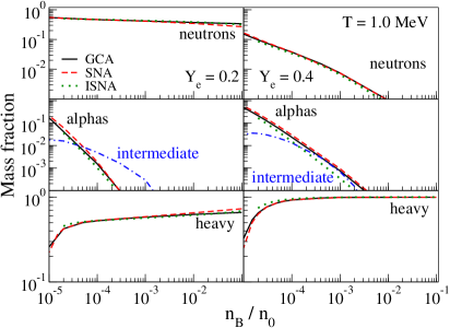
Figure 3.— Mass fractions associated with nuclei with $Z=0$, $Z=2$, $3\leq Z\leq 20$ (intermediate), and $Z>20$ (heavy), obtained employing the LDM1. The solid, dashed and dotted curves denote the predictions of GCA, SNA and ISNA calculations. Upper, middle and lower panels provide the mass fractions for neutrons, alpha particles and heavy nuclei. The dashed-dotted curves in the middle left and middle right panels denote the mass fractions in the GCA calculations due to nuclei with $2\leq Z\leq 20$, excluding alpha particles. The left panels give results for $Y_{e}=0.2$, and the right panels give results for $Y_{e}=0.4$. All panels are for $T=1.0$ MeV.

It may also be noticed that $n_{A}$ shows a broad distribution for all baryon densities displayed in the figure. The width becomes narrower as $n_{B}$ decreases, but it remains finite, for the reasons discussed above. The position of the peak of the distribution also shifts to lower values since dilute configurations favor partitions with higher numbers of free nucleons and light particles, which compete for the available charge and mass (equations (14) and (15)) against heavy nuclei.

This competition is illustrated in Figure 3, which shows the mass fraction associated with different particles. These results clearly reveal that more mass is contained in neutrons and alpha particles as one goes towards lower densities. The contribution from $Z=1$ is not presented since it is relatively small for the neutron rich systems we consider (even though it is included in our models). Consistent with the conclusions of earlier work (Epstein & Arnett, 1975; Burrows & Lattimer, 1984; Lattimer & Swesty, 1991), the mass fractions of alpha particles, heavy nuclei, and neutrons predicted by the GCA and SNA calculations are very similar, despite the non-negligible widths of the mass and charge distributions for the CGA calculations.

Similarly, the interactions between the gas particles and between the gas and the heavy nucleus included in the ISNA model make comparatively small differences to the mass fractions in Figure 3. The main differences appear to be that the ISNA model predicts somewhat smaller values for alpha particle and larger values for the neutron mass fractions compared to the SNA model. This partly reflects small differences between the mass formulae used in the SNA and ISNA models. In general, both models predict similar values for the the mass of the heavy nucleus at $Y_{e}=0.4$, but the heavy nucleus is somewhat lighter for the ISNA model at $Y_{e}=0.2$.

The qualitative dependence of $A_{\rm max}$ and $A_{h}$ on the electron fraction may be understood in terms of the symmetry energy. At small values of $Y_{e}$, neutrons are more abundant than protons and consequently, the neutron chemical potential exceeds the proton chemical potential. As a consequence, the number of free neutrons and the neutron mass fraction increase, as can be noticed from Figure 3, and nuclei also tend to have more neutrons than usual. Owing to the symmetry energy, an increase in the neutron number increases the binding energy of protons within a nucleus, the tendency for nuclei to have larger neutron number $N$ is accompanied by the distribution of heavy nuclei shifting to larger $A$ and $Z$ values. The increased neutron mass fraction at $Y_{e}=0.2$ can only be achieved if the heavy mass fraction correspondingly decreases. For this reason, the mass fraction associated with heavy nuclei is smaller for $Y_{e}=0.2$ compared with those obtained at $Y_{e}=0.4$.

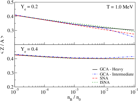
Figure 4.— Average $Z/A$ of heavy nuclei predicted by the GCA, SNA and ISNA models, using the LDM1, are shown by the solid, dashed and dotted lines, respectively. The dashed-dotted lines show the average $Z/A$ values for lighter nuclei with $3\leq Z\leq 20$ that lie below the heavy nucleus charge distribution.

At higher densities, the decrease in the free volume and corresponding increase in heavy nucleus mass means that the additional neutrons at $Y_{e}=0.2$ will be largely contained in the heavy nucleus. Thus the isotope composition of the heavy nucleus should be more sensitive to the baryon density when the matter is appreciably asymmetric. This aspect is illustrated in Figure 4, which shows the average value of $Z/A$ obtained with both models. As expected, it is fairly independent of $n_{B}$ for nearly symmetric matter, whereas it is quite sensitive to it at small values of $Y_{e}$. The predictions of the SNA model follow those made by the GCA fairly closely, at least at low densities. The SNA model tends to give more neutron rich heavy nuclei, partly because $A_{h}$ is systematically larger than $A_{\rm max}$ and the isobar with the highest binding energy in nuclear mass formulae is increasingly shifted towards the neutron rich side with increasing nuclear mass. Some of the extra neutrons in the GCA calculations are also contained in lighter intermediate mass nuclei with $3\leq Z\leq 20$ that lie below the heavy nucleus charge distribution.

The collapse of a supernova is accompanied by large changes in many properties of the system, such as the entropy, pressure, temperature, density, and energy (Bethe, 1990), some of which have an impact on the supernova dynamics. We therefore have evaluated the entropies and energies predicted by the GCA, SNA and ISNA models. The entropy may be obtained from these approaches through the standard thermodynamic relation

$$S=\log{Z_{G}}+T\left[\frac{\partial}{\partial T}\log Z_{G}\right]_{\mu,V}\;.$$ (43)

Applying the relationships in the preceding section, $S$ becomes

$$S=V\sum_{A,Z}n_{A,Z}\left[\frac{5}{2}+\frac{1}{T}(f_{A,Z}-\mu_{A,Z})-\frac{\partial f_{A,Z}}{\partial T}\right],$$ (44)

where

$$\frac{\partial f_{A,Z}}{\partial T}=-5\beta_{0}A^{2/3}\frac{TT_{c}^{2}}{(T_{C}^{2}+T^{2})^{2}}\left(\frac{T_{c}^{2}-T^{2}}{T_{c}^{2}+T^{2}}\right)^{1/4}-\frac{2A}{\epsilon_{0}}T\;.$$ (45)

The total energy of the system is given by

$$E=V\sum_{A,Z}n_{A,Z}\mu_{A,Z}+TS-PV.$$ (46)

The pressure $P$, which may be obtained from

$$P = T\left[\frac{\partial}{\partial V}\log Z_{G}\right]_{T,\mu}$$ (47)

$$= \frac{T}{\Omega}\sum_{A,Z}n_{A,Z}\left[1+\frac{1}{2}\frac{\Omega}{T}\frac{Z^{2}}{A^{1/3}}C_{c}u\right]$$

where

$$u=-\left(n_{B}/n_{0}\right)^{1/3}+\left(n_{B}/n_{0}\right)\;.$$ (48)

The second term in equation (47) is due to the Coulomb interaction between the electron gas and the nuclei and, therefore, is always negative for $n_{B}<n_{0}$.

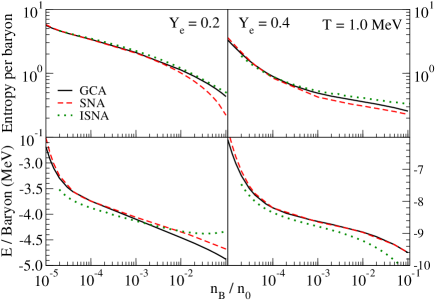
Figure 5.— Entropy and energy per baryon for different values of the baryon density, obtained using the LDM1. The solid, dashed and dotted lines denote the CGA, SNA and ISNA calculations respectively. The left panels are for $Y_{e}=0.2$ and the right panes are for $Y_{e}=0.4$.

The entropy and energy predicted by the GCA and SNA models are shown by the solid and dashed lines in Figure 5 for the same baryon densities and temperature used above. We do not show the nuclear pressure since, at these densities, it is much smaller than that of the electron gas (Bethe, 1990; Cooperstein, 1985) and, therefore, does not play a significant role. Although a fairly reasonable agreement is found for low densities $n_{B}<10^{-3}$, differences between GCA and SNA models can be found at higher densities where the GCA mass distributions become rather broad. The deviations between the SNA and ISNA results for the energy and entropy are relatively small, only a few tenths of an MeV for $Y_{e}=0.4$. However, there are larger deviations at $Y_{e}=0.2$ where the nuclei are extremely neutron rich.

The differences at higher densities and low $Y_{e}$ are not surprising: this is the region where one expects the results to depend sensitively on the details of the mass formula and information about the nuclear symmetry energy (Steiner, 2008). However, the differences at low density have a different origin: near $Y_{e}=0.2$ and $n_{B}/n_{0}=10^{-5}$, the free energy is very flat in the direction of the parameter space which determines the number of nuclei relative to the number of alpha particles. The reason for this is that the free energy can be minimized in one of two ways: (i) the system can choose to create more entropy (and thus decrease the free energy) by making a lot of alpha particles from nuclei, or (ii) the system can choose to create nuclei from alpha particles because the extra binding created by nuclei will also decrease the free energy. Within the ISNA model one can vary the number density of nuclei by 70 %, and this modification only changes the free energy by 0.1 %, while changing the entropy by 10 %. Because the free energy is so flat, the entropy in this region is quite sensitive to the nuclear mass formula. Fortunately this low-density, low-$Y_{e}$ region is not actually probed frequently in actual supernova simulations.

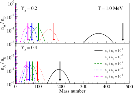
Figure 6.— Same quantities as in Figure 2. In this figure, however, the results are obtained using the LDM2 mass model.

In order to verify the extent to which our conclusions depend on treatment of the nuclear symmetry energy in the liquid drop formula used in these statistical treatments, we have also carried out GCA and SNA calculations using the LDM2 formula presented in Sect. 2.1. The corresponding isobar number densities are shown in Figure 6. Qualitatively, the calculations in Figure 6 resemble those in Figure 2 obtained using the LDM1 formula. Quantitatively, there are differences, however. Most notably, the discrepancies between the GCA and SNA model predictions are now much larger for LDM2 than for LDM1, particularly for $Y_{e}=0.2$, at $n_{B}/n_{0}=0.1$. This is due to the lack of a surface symmetry energy term in the LDM2 mass model. The resulting under prediction of the binding energies for light masses in the LDM2 formulae shifts mass of the maximum $A_{\rm max}$ for the GCA distribution towards larger values, where the difference between $A_{\rm max}$ and $A_{h}$ values is typically much larger. Nevertheless, the mass fractions predicted using the LDM2 mass model (not shown) are similar to those shown in Figure 3, except that intermediate mass nuclei ($3\leq Z\leq 20$) give a somewhat larger contribution for the LDM2 to the mass fraction at the lowest density.

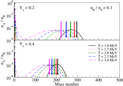
Figure 7.— Same as Figure 2, except that the baryon density is fixed and the temperature is varied from 1 to 3 MeV.

The discrepancies between the predictions of the treatments are more pronounced at the highest baryon density. To illustrate the dependence on temperature there, we compare the two calculations at $n_{B}/n_{0}=0.1$ for temperatures ranging from 1 to 3 MeV, values that are in the range relevant to supernova studies. The isobar number densities, obtained using the LDM1, are shown in Figure 7. Reflecting the larger phase-space accessible to the system at higher temperatures, the GCA isobar distributions become broader, the value of $A_{\rm max}$ decreases, and a larger fraction of the mass is in the form of nucleons or light nuclei at higher temperatures. The trend of increasing nucleon yields with temperature is also exhibited by the SNA model, but the discrepancies between the GCA and SNA approaches become larger as $T$ and the widths of the mass distributions increase. In spite of the larger width of the isobar distributions, however, the mass fractions obtained with GCA and the SNA model (not shown) agree to within $15\%$ for $Y_{e}=0.4$ and to within about $25\%$ for $Y_{e}=0.2$. The intermediate mass nuclei have a slightly larger mass fraction, but not enough to significantly change the mass fraction associated with heavy nuclei.

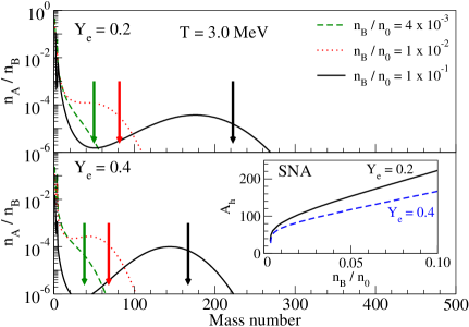
Figure 8.— Same as Figure 7, except that the $T=3$ MeV. The inset shows values for $A_{\rm h}$ calculated within the SNA model as a function of the density.

Figure 8 shows the complementary comparison between the GCA and SNA calculations using the LDM1 as a function of density at $T=3~{}\mathrm{MeV}$. We do not compare the two calculations below $n/n_{0}=4\times 10^{-3}$ because at this temperature the mass $A_{h}$ of the most probable heavy nucleus drops to zero below this density. The inset in the figure shows the detailed dependence of $A_{h}$ predicted by the SNA model. Even though, some heavy nuclei are predicted by the GCA model at $n/n_{0}<4\times 10^{-3}$, the mass fraction of $Z>20$/$A>50$ at such densities is small and of the order of $3-6\times 10^{-2}$. Both Figure 7 and Figure 8 show that the discrepancies between the GCA and SNA calculations increase with density over the range of densities investigated in this work.

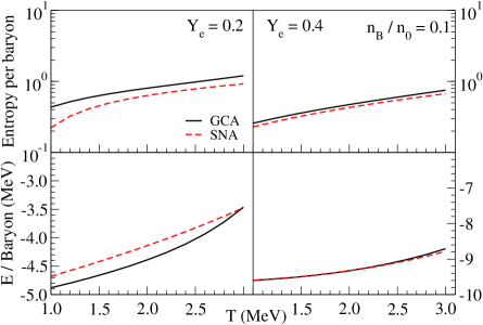
Figure 9.— Same quantities as plotted in Figure 5, except that the baryon density is fixed at $\rho/\rho_{0}=0.1$ and the temperature is varied from 1 to 3 MeV.

In general, the agreement between the GCA and SNA approaches is somewhat better at $Y_{e}=0.4$ than at $Y_{e}=0.2$ where the mass distributions are wider. This conclusion also holds for the thermodynamic variables. The dependence of the entropy and energy per baryon on the temperature is shown at a fixed density of $n=0.1n_{0}$ in Figure 9. Clear differences between the GCA and SNA calculations are predicted for $Y_{e}=0.2$. There the entropy difference ($\Delta S/A\approx 0.2$) remains roughly constant as a function of temperature. The larger mass in the SNA leads to a lower energy baryon in the SNA than in the GCA calculation. The energy difference reaches its largest value ($\Delta E/A\approx 0.15$ MeV) at $T=1$ MeV. This difference decreases with temperature to a negligible value at $T=3$ MeV. In contrast, the differences between GCA and SNA calculations are comparatively small for $Y_{e}=0.4$, reflecting the smaller widths of the heavy mass distributions at $Y_{e}=0.4$.

The complementary density dependencies of the entropies and energies for GCA and SNA calculations at $T=3$ MeV are shown in Figure 10. For both $Y_{e}=0.2$ and $Y_{e}=0.4$, the largest differences between the energies of SNA and are actually observed at $n/n_{0}\approx 0.01$. The entropy differences generally increase with density for both $Y_{e}=0.2$ and $Y_{e}=0.4$. Both entropy and energy differences are larger for $Y_{e}=0.2$ than for $Y_{e}=0.4$, reflecting the larger widths of the heavy nucleus mass distributions at $Y_{e}=0.2$. Both Figs. 9 and 10 demonstrate that the wide mass distributions of the GCA calculations at densities of $n/n_{0}\sim 0.01-0.1$ lead to non-negligible differences between the entropies and energies predicted by the GCA and SNA approaches. The ISNA results are similar, again showing larger deviations from SNA calculations in the neutron rich case at $Y_{e}=0.2$. The density range over which results are available is slightly smaller because the disappearance of the heavy nucleus occurs as a higher density in the ISNA model. The transition from heterogeneous to homogeneous matter, especially in neutron-rich matter, is very model dependent.

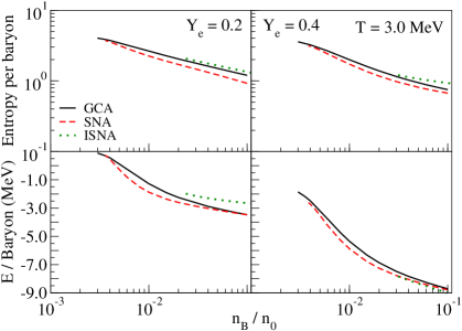
Figure 10.— Same as Figure 5, except that the temperature is fixed at $T=3$ MeV and the baryon density is varied.

Finally, to provide one more example of the importance of the mass formula, we show, in Figure 11, the mass distributions predicted by the GCA for the LMD2 mass formula in comparison to the corresponding SNA predictions. We find that there are larger discrepancies between the GCA and SNA predicted for the LDM2 parametrization than for the LMD1 parametrization. As the mass fractions and the thermodynamic variables obtained in this case are very similar to those obtained for the LDM1 parametrization, we do not show them in the interest of brevity. Comparing the predictions in two different parameterizations of the nuclear symmetry in Figure 11, we find that the changes in the mass distributions due to inclusion of the surface symmetry energy correction are less significant than the predicted differences between the GCA and SNA calculations that use the same liquid drop mass model (and same symmetry energy).

In principle, nuclei must have a surface symmetry energy term. The magnitude of the surface symmetry energy coefficient, however, is not well constrained by the measured nuclear masses (Danielewicz, 2003). Even though the differences between the GCA and SNA calculations exceed the differences between the LDM1 and LDM2 calculations, parameterizations for the density dependence of the symmetry energy may be chosen that predict much larger effects (Botvina & Mishustin, 2005). Ideally, a general investigation of the role of the symmetry energy in the supernovae EOS should include both an assessment of the sensitivity of the mass distributions to the choice of the symmetry energy as well as an assessment of whether the chosen form is consistent with known experimental information (Souza et al., 2008). A systematic investigation of the effect of the symmetry energy in relationship to the current experimental information is in preparation.

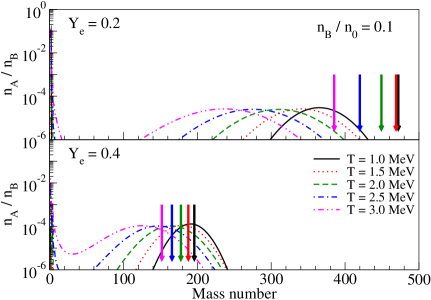
Figure 11.— Same as Figure 7, except that the LDM2 is used in the calculations.

4. Concluding Remarks

This work has focused on the differences between the Grand Canonical Approximation and simplified Single Nucleus Approximation utilized in most supernova calculations. Consistent with the earlier work in Burrows & Lattimer (1984), we find that the thermodynamic functions are relatively well described by the SNA at densities below $0.01\rho_{0}$. At higher densities, differences emerge that can be traced to the large widths of the GCA mass distributions. We have compared the simple SNA model to a more elaborate ISNA model that considers effects that become relevant at higher densities, such as the interactions between gas particles. We find differences between the SNA and ISNA models of these average quantities that are comparable to the differences between the GCA and SNA calculations. This indicates the importance of taking such effects into account accurately. Comparisons of the GCA, SNA and ISNA models suggest that the error made by assuming a single nucleus in the energies and entropies per baryon may be comparable to or smaller than the other uncertainties in the problem, such as the nuclear mass formulae and the inclusion of quantum statistics and interactions between gas particles.

Large differences can be found between the GCA predictions for the the masses of nuclei and those of the SNA and ISNA calculations. Single nucleus approximations, in general, tend to predict much larger heavy nucleus masses than does the GCA. Considering first the differences between GCA and SNA calculations, we find that the SNA model systematically overpredicts the mass number of nuclei that are actually present in the more accurate GCA model because it neglects the contribution from lighter nuclei and the large width of the mass distribution. This discrepancy grows with increasing temperature. Such a large difference in nuclear distributions is significant. Even though some regimes (particularly higher densities and lower temperatures) are affected by quantum statistics, our calculations indicate that the effects of assuming a distribution of nuclei rather than a sole representative nucleus are much larger and sufficiently robust. This suggests that first explorations of the consequences on supernova simulations of these differences using classical models of non-interacting nuclei may be helpful and should be performed.

These results has specific implications for the equation of state tables and the weak interaction physics inputs used as inputs for supernova simulations. Our work suggests that tables utilizing the SNA can be updated to include nuclear distributions by applying an appropriate GCA model. We are exploring such issues with the aim of determining their impact on the weak interaction rates (Janka et al., 2007) in supernova simulations. The use of a GCA model will also allow future investigations to more accurately determine the neutrino spectra because it directly handles light nuclei, the importance of which was emphasized in Arcones et al. (2008).

References

- Aguiar et al. (2006) Aguiar, C. E., Donangelo, R., & Souza, S. R. 2006, Phys. Rev. C, 73, 024613
- Akmal et al. (1998) Akmal, A., Pandharipande, V. R., & Ravenhall, D. G. 1998, Phys. Rev. C, 58, 1804
- Arcones et al. (2008) Arcones, A., Martinez-Pinedo, G., O’Connor, E., Schwenk, A., Janka, H.-T., Horowitz, C. J., & Langanke, K. 2008, arXiv.org:0805.3752
- Audi & Wapstra (1995) Audi, G. & Wapstra, A. H. 1995, Nucl. Phys., A595, 409
- Baym et al. (1971) Baym, G., Bethe, H. A., & Pethick, C. J. 1971, Nucl. Phys., A175, 225
- Bethe (1990) Bethe, H. A. 1990, Rev. Mod. Phys., 62, 801
- Bethe et al. (1979) Bethe, H. A., Brown, G. E., Applegate, J., & Lattimer, J. M. 1979, Nucl. Phys. A, 324, 487
- Bhattacharyya & Mekjian (1999) Bhattacharyya, P. & Mekjian, S. Das Gupta. A. Z. 1999, Phys. Rev. C, 60, 054616
- Bondorf et al. (1995) Bondorf, J. P., Botvina, A. S., Iljinov, A. S., Mihustin, I. N., & Sneppen, K. 1995, Phys. Rep., 257, 133
- Botvina & Mishustin (2005) Botvina, A. & Mishustin, I. N. 2005, Phys. Rev. C, 72, 048801
- Botvina & Mishustin (2004) Botvina, A. S. & Mishustin, I. N. 2004, Phys. Lett. B, 584, 233
- Burrows & Lattimer (1984) Burrows, A. & Lattimer, J. M. 1984, Ap. J, 285, 294
- Cooperstein (1985) Cooperstein, J. 1985, Nucl. Phys., A438, 722
- Danielewicz (2003) Danielewicz, P. 2003, Nucl. Phys., A727, 233
- Epstein & Arnett (1975) Epstein, R. I. & Arnett, W. D. 1975, Ap. J, 201, 202
- Hix et al. (2003) Hix, W. R., Messer, O. E. B., Mezzacappa, A., Liebendoörfer, M., Sampaio, J., Langanke, K., Dean, D. J., & Martinez-Pinedo, G. 2003, Phys. Rev. Lett., 91, 201102
- Janka et al. (2007) Janka, H.-T., Langanke, K., Marek, A., Martínez-Pinedo, G., & Müller, B. 2007, Phys. Rep., 442, 38
- Lattimer et al. (1985) Lattimer, J. M., Pethick, C. J., Ravenhall, D. G., & Lamb, D. Q. 1985, Nucl. Phys. A, 432, 646
- Lattimer & Swesty (1991) Lattimer, J. M. & Swesty, F. D. 1991, Nucl. Phys., A535, 331
- Prakash et al. (1997) Prakash, M., Bombaci, I., Prakash, M., Ellis, P. J., & Lattimer, J. M. 1997, Phys. Rep., 280, 1
- Preston & Bhaduri (1975) Preston, M. A. & Bhaduri, R. K. 1975, Structure of the Nucleus (Addison-Wesley, Reading, MA)
- Ravenhall et al. (1972) Ravenhall, D. G., Bennett, C. D., & Pethick, C. J. 1972, Phys. Rev. Lett., 28, 978
- Ravenhall et al. (1983) Ravenhall, D. G., Pethick, C. J., & Wilson, J. R. 1983, Phys. Rev. Lett., 50, 2066
- Shen et al. (1998) Shen, H., Toki, H., Oyamatsu, K., & Sumiyoshi, K. 1998, Nucl. Phys. A, 637, 435
- Souza et al. (2003) Souza, S. R., Danielewicz, P., Das Gupta, S., Donangelo, R., Friedman, W. A., Lynch, W. G., Tan, W. P., & Tsang, M. B. 2003, Phys. Rev. C, 67, 051602(R)
- Souza et al. (2008) Souza, S. R., Tsang, M. B., Donangelo, R., Lynch, W. G., & Steiner, A. W. 2008, Phys. Rev. C, 78, 014605
- Steiner (2008) Steiner, A. W. 2008, Phys. Rev. C, 77, 035805
- Sumiyoshi et al. (2005) Sumiyoshi, K., Yamada, S., Suzuki, H., Shen, H., Chiba, S., & Toki, H. 2005, ApJ, 629, 922
- Tan et al. (2003) Tan, W. P., Souza, S. R., Charity, R. J., Donangelo, R., Lynch, W. G., & Tsang, M. B. 2003, Phys. Rev. C, 68, 034609
- Wigner & Seitz (1934) Wigner, E. & Seitz, F. 1934, Phys. Rev., 46, 509