Transport and localization in periodic and disordered graphene superlattices.

Abstract

We study charge transport in one-dimensional graphene superlattices created by applying layered periodic and disordered potentials. It is shown that the transport and spectral properties of such structures are strongly anisotropic. In the direction perpendicular to the layers, the eigenstates in a disordered sample are delocalized for all energies and provide a minimum non-zero conductivity, which cannot be destroyed by disorder, no matter how strong this is. However, along with extended states, there exist discrete sets of angles and energies with exponentially localized eigenfunctions (disorder-induced resonances). Owing to these features, such samples could be used as building blocks in tunable electronic circuits. It is shown that, depending on the type of the unperturbed system, the disorder could either suppress or enhance the transmission. Remarkable properties of the transmission have been found in graphene systems built of alternating p-n and n-p junctions. The mean transmission coefficient has anomalously narrow angular spectrum, practically independent of the amplitude of the fluctuations of the potential. To better understand the physical implications of the results presented here, most of these have been compared with the results for analogous electromagnetic wave systems. Along with similarities, a number of quite surprising differences have been found.

I Introduction.

The exploration of graphene is nowadays one of the most animated areas of research in condensed matter physics (see, e.g., Refs.Katsnelson2 ; Geim ; periodic-1 ). Its unique properties not only arouse pure scientific curiosity but also suggest possible practical applications. More in-depth studies of graphene continuously bring about more counterintuitive discoveries. Examples are plentiful. Suffice to mention a novel integer quantum Hall effect dis-exp-1 ; Castro , total transparency of any potential barrier for normally-incident electrons/holes Katsnelson1 (in analogy with the Klein paradox Klein ), and the recently predicted focusing of electron flows by a rectangular potential barrier Cheianov (an analog of the Veselago lens Veselago ; Pendry ). Of even greater surprise are the properties of disordered graphene systems disorder-1 ; disorder-2 ; Titov-1 ; San-Jose ; disorder-3 ; disorder-4 ; dis-exp-2 ; dis-exp-3 . The latest results, both theoretical and experimental, led to the amazing conclusion that there is no localization in disordered graphene, even in the one-dimensional situation, i.e., when the random potential depends only on one coordinate. In this paper, we show that this conclusion, if taken unreserved, could be misleading. We demonstrate here that a well-pronounced localization can take place in graphene, i.e., there could exist a (quasi)-discrete spectrum with exponentially localized eigenfunctions remark-1 . This localization can occur even though disorder can never make a graphene sample a complete insulator, and there is always a minimal residual conductivity (an indication of delocalization). In this paper, the charge transport in periodically and randomly layered graphene structures is studied and analogies with the propagation of light in layered dielectrics are discussed.

II Basic equations

II.1 Charge transport in graphene

A graphene layer consists of two triangular sublattices (A and B). The low-energy band is gapless and electronic states are found near two (electron and hole) cones. The behavior of charge carriers (electrons and holes) near the Dirac point is governed by the 2D Dirac equation Slonczewski ; Semenoff :

$$v_{F}\left(\mathbf{\vec{\sigma}\cdot\hat{p}}\right)\Psi=(E-V)\Psi,$$ (1)

where $\Psi$ is a two-component spinor $(\Psi_{A},\Psi_{B})^{T}$, the components of a pseudospin matrix $\vec{\sigma}$ are given by Pauli’s matrices, $\mathbf{\hat{p}}$ is the momentum operator, $v_{F}$ is the Fermi velocity, $V(x,y)$ is the potential, and $E$ is the state energy. When the potential depends on one coordinate, $V=V(x)$, the wave function $\Psi(x,y)$ can be written as $\Psi(x,y)=e^{ik_{y}y}\psi(x)$, and Eq. (1) can be presented in the dimensionless form

$${\frac{d\psi_{A}}{d\xi}}-\beta\psi_{A} = i[\varepsilon-u(\xi)]\psi_{B},$$

$${\frac{d\psi_{B}}{d\xi}}+\beta\psi_{B} = i[\varepsilon-u(\xi)]\psi_{A}.$$ (2)

Here $\xi=x/d$, $d$ is the characteristic spatial scale of the potential variations, $\varepsilon=Ed/\hbar v_{F}$, $u=Vd/\hbar v_{F}$, and $\beta=k_{y}d$.

In what follows, we consider potentials $u(\xi)$ comprised of periodic or random chains of rectangular barriers depicted in Fig. 1

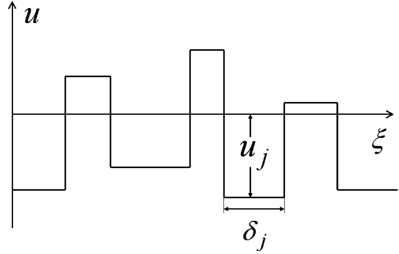
Figure 1: Schematic diagram of the potential $u(\xi)$.

In a $j$-th layer, the solution of Eq. (II.1) has the form: $\psi_{(A,B)_{j}}=\psi_{(A,B)_{j}}^{(+)}e^{i\kappa_{j}\xi}+\psi_{(A,B)_{j}}^{(-)}e^{-i\kappa_{j}\xi}$, where $\kappa_{j}=\sqrt{(\varepsilon-u_{j})^{2}-\beta^{2}}$, $\psi_{(A,B)_{j}}^{(\pm)}$ are the amplitudes of the rightward $(+)$ and leftward $(-)$ propagating spinor components. At the layer interfaces the amplitudes $\psi_{(A,B)_{j}}^{(\pm)}$ and $\psi_{(A,B)_{j+1}}^{(\pm)}$ are connected by the equation

$$\psi_{(A,B)_{j+1}}^{(+)}+\psi_{(A,B)_{j+1}}^{(-)}=\psi_{(A,B)_{j}}^{(+)}+\psi_{(A,B)_{j}}^{(-)},$$ (3)

which follows from the continuity of the spinor components. Since from Eq. (II.1) the amplitudes $\psi_{(A,B)_{j}}^{(\pm)}$ are connected,

$$\psi_{B_{j}}^{(\pm)}=c_{j}^{(\pm)}\psi_{A_{j}}^{(\pm)},\hskip 8.53581ptc_{j}^{(\pm)}={\frac{i\beta\pm\kappa_{j}}{\varepsilon-u_{j}}},$$ (4)

$$c_{j}^{(\pm)}={\frac{i\beta\pm\kappa}{\sqrt{\beta^{2}+\kappa^{2}}}}\mathrm{sgn}(\varepsilon-u_{j})=\pm e^{\pm i\theta_{j}}\cdot\mathrm{sgn}(\varepsilon-u_{j}),$$ (5)

we will only consider the amplitudes $\psi_{A}^{(\pm)}$ and omit the subscript “A”. If $\mathrm{Im}\kappa_{j}=0$, $\theta_{j}=\arctan(\beta/\kappa_{j})$ is the angle between the wave vector $\mathbf{k}$ of the $(+)$ wave and the normal to the interface between the $j$-th and $\ (j+1)$-th layers (i.e., the angle of propagation in the $j$-th layer). Using Eqs. (3) and (4) one can calculate the matrix $\hat{M}_{j,j+1}$ that connects the amplitudes $\psi_{j}^{(\pm)}$ and $\psi_{j+1}^{(\pm)}$ on two sides of the interface, $\left(\psi_{j+1}^{(+)},\psi_{j+1}^{(-)}\right)^{T}=\hat{M}_{j,j+1}\left(\psi_{j}^{(+)},\psi_{j}^{(-)}\right)^{T}$:

$$\hat{M}_{j,j+1}={\frac{1}{2\cos\theta_{j+1}}}\left\|\begin{array}[]{cc}g_{j,j+1}^{(+)}&g_{j,j+1}^{(-)}\\ (g_{j,j+1}^{(-)})^{\ast}&(g_{j,j+1}^{(+)})^{\ast}\end{array}\right\|,$$ (6)

where

$$g_{j,j+1}^{(\pm)}=e^{-i\theta_{j+1}}\pm e^{\pm i\theta_{j}}\cdot\mathrm{sgn}[(\varepsilon-u_{j})(\varepsilon-u_{j+1})],$$ (7)

and $T$ denotes transposed vector.

The spinor components at the left and right boundaries of the $j$-th layer are connected by the diagonal matrix $\hat{S}_{j}=\mathrm{diag}(e^{i\alpha_{j}},e^{-i\alpha_{j}})$, where $\alpha_{j}=\kappa_{j}\delta_{j}$ is the phase accumulated by the wave propagating through the layer of the thickness $\delta_{j}$. Thus, the matrix $\hat{S}_{j+1}\hat{M}_{j,j+1}$ transports the spinor components from the left side of the interface between the $j$-th and $(j+1)$-th layers to the left side of the next interface between the $(j+1)$-th and $(j+2)$-th layers (see Fig. 2). Obviously, the total transfer matrix of a layered sample consisting of $N$ layers is given by the product of $\hat{S}\hat{M}$ matrices:

$$\hat{T}=\prod\limits_{j=0}^{N}\hat{S}_{j+1}\hat{M}_{j,j+1}$$ (8)

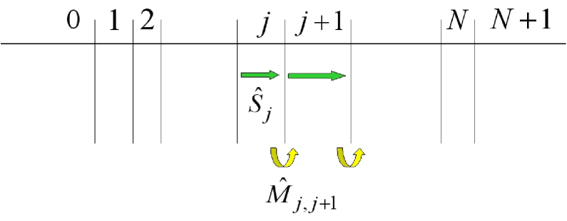
Figure 2: (color online) Propagation through a layered structure. The matrix $\hat{S}_{j}$ propagates through $j-$th layer (green arrow) and the matrix $\hat{M}_{j,j+1}$ connects the spinor amplitudes across the interface between $j$-th and $(j+1)$-th layers.

II.2 Light transport in dielectrics

Analogous products of matrices have been well studied in the context of transport of electromagnetic waves in layered media (see, for example, matrices and references therein). To better understand the physics of charge transport in graphene subject to a coordinate-dependent potential, in what follows, we contrast the results for graphene with those for the propagation of light in layered dielectric media (for more analogies between quantum and optical systems, see, e.g. Ref.Dragoman ; analogy ). Additional analogies, not discussed here, also exist with the transport and localization of phonons in different kinds of periodic and random one-dimensional structures Nori ; Nori_1 ; Nori_2 .

In the latter case, the matrices $\hat{S}_{j}$ are the same as in Eq. (8), and the transfer matrix, $\hat{\mathcal{M}}_{j,j+1}$,

$$\hat{\mathcal{M}}_{j,j+1}={\frac{1}{2\cos\theta_{j+1}}}\left\|\begin{array}[]{cc}\mathcal{G}_{j,j+1}^{(+)}&\mathcal{G}_{j,j+1}^{(-)}\\ (\mathcal{G}_{j,j+1}^{(-)})^{\ast}&(\mathcal{G}_{j,j+1}^{(+)})^{\ast}\end{array}\right\|,$$ (9)

that describes the transformation of the amplitudes of the electromagnetic waves at the interface between $j$th and $\ (j+1)$th layers, has the form Eq. (6) with $g_{j,j+1}^{(\pm)}$ being replaced by

$$\mathcal{G}_{j,j+1}^{(\pm)}=\cos\theta_{j+1}\pm\cos\theta_{j}\cdot\mathrm{sgn}(n_{j}n_{j+1}){\frac{Z_{j+1}}{Z_{j}}}$$ (10)

for $s$-polarized waves and

$$\mathcal{G}_{j,j+1}^{(\pm)}={\frac{Z_{j+1}}{Z_{j}}}\cos\theta_{j+1}\pm\cos\theta_{j}\cdot\mathrm{sgn}(n_{j}n_{j+1})$$ (11)

for $p$-polarized waves. Here, $\theta_{j}$ is the angle of the propagation, $Z_{j}=\sqrt{\mu_{j}/\varepsilon_{j}}$ is the impedance of $\ j$th layer, and $n_{j}=\pm\sqrt{\varepsilon_{j}\mu_{j}}$ is its refractive index. The signs $\pm$ correspond, respectively, to dielectrics with positive (right-handed, R) and negative (left-handed, L) refractive indices.

It is easy to see that the parameter $(\varepsilon-u)$ plays, in graphene, the same role as the refractive index $n$ in a dielectric medium. It is due to this similarity that a p-n junction (interface between regions where the values $(\varepsilon-u)$ have opposite signs) focuses charge carriers in graphene, like an R-L interface focuses electromagnetic waves Cheianov .

Note that in Eq. (7) (for graphene) there is no factor $Z_{j+1}/Z_{j}$, which determines the reflection coefficients at the boundary between two dielectrics born wolf . This means that the charge transport in graphene is similar to the propagation of light in a stack of dielectric layers with equal impedances. In particular, both p-n and p-p junctions are transparent for normally incident charged particles Cheianov ; Katsnelson1 . This property is readily seen from the analysis of the matrix $\hat{M}$: at $\beta=0$ it is a Pauli matrix $\hat{M}=\sigma_{x}$ for p-n junctions and unit matrix for p-p junctions. Therefore, a $(+)$-wave is totally transformed into a $(-)$-wave at a p-n junction, and remains a $(+)$-wave at a p-p junction. Another important difference between the transfer matrices $\hat{M}$ (graphene) and $\hat{\mathcal{M}}$ (electromagnetic waves) is that $\hat{M}$ is, generally speaking, a complex-valued matrix, while the $\hat{\mathcal{M}}$ is always real. As it is shown bellow, this distinction brings about rather peculiar dissimilarities between the conductivity of graphene and the transparency of dielectrics.

III Transport in periodic structures

Among the vast amount of publications on graphene, a significant and ever increasing part belongs to papers devoted to the charge transport in graphene superlattices formed by a periodic external potential (see, e.g., periodic-1 ; periodic-2 ; periodic-3 ; periodic-4 ; periodic-5 ). This is not only due to its theoretical interest but also because of the possibility of experimental realization and potential applications periodic-4 . In Ref. periodic-1 , for example, it was suggested that, by virtue of the high anisotropy of the propagation of carriers through graphene subjected to a Kronig–Penney type periodic potential, such a structure could be used for building graphene electronic circuits from appropriately engineered periodic surface patterns.

Here we consider a layer of graphene under a periodic alternating potential $u=\pm U_{0}$ and assume that $\varepsilon=0$. Two layers, $u_{1}=U_{0}$ and $u_{2}=-U_{0}$ with thicknesses $\delta_{1}$ and $\delta_{2}$, respectively, constitute the superlatice period with transfer matrix $\hat{T}=\hat{S}_{2}\hat{M}_{2,1}\hat{S}_{1}\hat{M}_{1,2}.$ Its eigenvalues $\lambda(\beta)$ indicate whether this periodic structure is transparent or not. Namely, the structure is transparent when $|\lambda(\beta)|$ $=1\$and is opaque when $|\lambda(\beta)|$ $\neq 1$. Note that analogous ($n_{1}=-n_{2}$) L-R periodic dielectric structures are transparent at all angles of incidence when $Z_{1}=Z_{2}.$ In contrast, a periodic array of p-n junctions in graphene has a rather nontrivial angular dependence of the transmission coefficient $T(\beta)$. This distinction between periodic graphene and dielectric lattices follows from the difference in the corresponding transfer matrices: $\hat{M}$ is complex-valued while $\hat{\mathcal{M}}$ is real.

If $\varepsilon=0$ and $\delta_{1}=\delta_{2}\equiv\delta$ (symmetric graphene system) the equation for the eigenvalues of the matrix $\hat{T}$ has the form

$$\lambda^{2}-2\lambda{\frac{1-\sin^{2}\theta\cos 2\alpha}{\cos^{2}\theta}}+1=0,$$ (12)

where $\alpha=\kappa(\theta)\delta$. It is easy to see that $|\lambda|=1$ at normal incidence $(\theta=0)$ and at a discrete set of angles, $\theta_{m},$ given by

$$\alpha(\theta_{m})=m\pi,\hskip 8.53581ptm=\pm 1,\pm 2,\ldots$$ (13)

Although the eigenvalues $\lambda(\beta)$ are well defined for an infinite system, they are also quite meaningful for a sufficiently long finite periodic sample: at $\theta_{m}$ there are maxima of the transmission coefficient $T(\beta).$ The transmission coefficient $T(\beta)$ of the symmetric graphene structure is presented in Fig. 3a. a similar transmission spectrum $T(\beta)$ exists at $\theta\neq 0$ in L-R periodic structures (Fig. 3b) made of layers with equal absolute values of the refractive indexes, $n_{1}=-n_{2}$, and different impedances $Z_{1}\neq$ $Z_{2}$ Wu1 ; Wu2 . The transmission coefficient $T(\beta)$ for a symmetric periodic R-R system is shown in Fig. 3c.

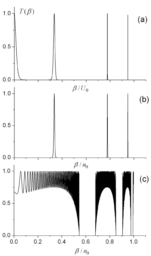
Figure 3: Transmission coefficient $T(\beta)$ for: (a) graphene subject to a symmetric periodic potential $u=\pm U_{0}$; (b) a symmetric periodic L-R dielectric structure; (c) a symmetric periodic R-R dielectric structure. The parameter $U_{0}$ plays in graphene the same role as the refractive index $n_{0}$ in a dielectric medium. For (b) and (c), $n_{0}=U_{0}$ and $Z_{1}/Z_{2}=1.1$. In all figures, L stands for left-handed media and R for right-handed media. Thus, the structures considered in (b) are periodic stacks LRLRLR…of dielectrics. The structures considered in (c) are periodic RRRRRR…stacks of dielectrics.

The transmission spectrum $T(\beta)$ in Fig. 3a, which consists of a discrete set of incidence angles, is the result of the degeneracy caused by the high symmetry of the structure ($u_{1}=-u_{2}$, $\varepsilon=0$, and $\delta_{1}=\delta_{2}$). Any symmetry-breaking splits the degeneracy and the spectrum takes the form usual for ordinary periodic structures: a set of conducting zones of non-zero width separated by band gaps periodic-2 . In Fig. 4a, the zone structure of the transmission spectrum is shown. It is important to note that instead of the wave number $k_{y}$ and the energy, typically used in zone diagrams, the variables in Fig. 4a are the asymmetry parameter $\Delta=(\delta_{1}-\delta_{2})/2$ and $\beta=kd\sin\theta,$ respectively. Note that even in non-symmetric structures there are some values of $\delta_{1}$ and $\delta_{2}$ for which, along with the usual conducting zones and band gaps, there exists a discrete set of resonant $\beta$s. Note also that, for a fixed $\Delta$, the transmission zones as a function of $\beta$ are very narrow, making the direction of the charge flux easily tunable by changing the applied voltage $U_{0}$.

Figure 4: (color online) Transmission coefficient $T(\beta,\Delta)$ as a function of the difference of the thicknesses of two layers, $\Delta=(\delta_{1}-\delta_{2})/2$, and of the normalized parameter $\beta=k_{y}d\equiv kd\sin\theta$ for: (a) periodic graphene subject to an alternating periodic potential; (b) periodic L-R dielectric structure; (c) periodic R-R dielectric structure. In (a), the normalization parameter $U_{0}$ is the dimensionless applied voltage; in (b) and (c), the normalization parameter $n_{0}$ is the refraction index in a dielectric medium, and $Z_{1}/Z_{2}=1.1$. The grey area corresponds to a perfect transmission, $T=1$. The white regions correspond to $T=0$.

For comparison, the analogous spectra for L-R and R-R periodic structures with $|n_{1}|=|n_{2}|$ and $Z_{1}\neq Z_{2}$ are presented in Fig. 4b,c. One can see there that the transmission coefficients of graphene and L-R structures are similar, and both differ drastically from that of the R-R structure.

A phenomenon similar to the total internal reflection of light can occur to charge in graphene at a non-symmetric p-n interface when $|\varepsilon-u_{1}|\neq|\varepsilon-u_{2}|$ (here $u_{1}$ and $u_{2}$ are the potentials on either side of the interface). However, a periodic set of such junctions is transparent for some angles of incidence periodic-2 . This effect is similar to photon tunneling (frustrated total internal reflection) in stacks of dielectric layers Dragila .

Let us now consider the transmission of charge through a single non-symmetric p-n junction, assuming that $u_{1}=-u_{2}=U_{0}\geq\epsilon>0$. Then, if $(\varepsilon-U_{0})^{2}<\beta^{2}<(\varepsilon+U_{0})^{2}$, a total internal reflection occurs at the interface; however there are ranges of the angle of incidence where the system is transparent. An example of such an angular spectrum is shown in Fig. 5a.

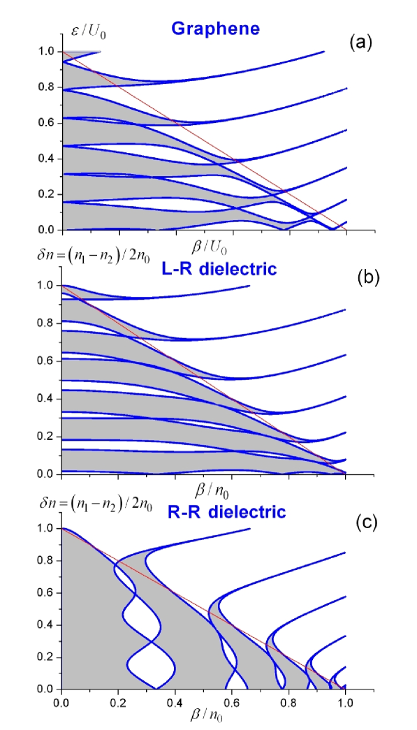
Figure 5: (color online) Transmission coefficient $T(\beta)$ for: (a) periodic graphene subject to an alternating potential; (b) periodic L-R dielectric structure; (c) periodic R-R dielectric structure. The coordinates and the colors are the same as in Fig. 4. In the region above the straight line the condition of total internal reflection is satisfied.

Physically, the tunneling conductance (proportional to the transmission coefficient) is due to the confined states in graphene quantum well Pereira ; RIKEN . Although the confined states in a single quantum well have a discrete spectrum $\beta=\beta_{n}(\varepsilon)$, an infinite periodic chain of wells, interacting via their evanescent wave functions, forms transmission bands centered around $\beta_{n}$.

Periodic L-R and R-R dielectric structures have properties similar to the properties described in this subsection for graphene. Figures 5b,c show the transmission spectrum of L-R and R-R structures with a period composed of two blocks with equal thicknesses and different refractive indexes, $|n_{1}|=1+\delta n$ and $|n_{2}|=1-\delta n$.

IV Transmission in disordered structures

Based on the results obtained for ideally periodic systems, the authors of Ref. periodic-1, ; periodic-4, suggested that graphene superlattices could be used as tunable elements in electronic devices. Since parameters of such structures are extremely sensitive to the variations of the applied potential it is worthwhile to study the effect of disorder (random deviations of the potential from periodicity) on the propagation of charge in such configurations. Moreover, this study is of interest by itself because strongly disordered (with no periodic component) potentials bring about further unexpected spectral and transport properties of graphene samples, which make them potentially useful as an alternative to pure periodic systems.

A surprising and counter-intuitive result is that a sample of graphene subject to a random one-dimensional potential, $u(x),$ is absolutely transparent to the charge flow perpendicular to the $x$-direction, no matter how long is the sample and how strong the disorder isTitov-1 . This means that in such samples there exists a minimal non-zero conductivity, which (together with symmetry and spectral flow arguments) led to the conclusion that there is no localization in 1D disordered graphene systems Titov-1 ; Koshino . However, this statement (being correct in some sense) should be perceived with a certain caution. Below, we show that although the wave functions of normally incident particles are extended and belong to the continuous part of the spectrum, away from some vicinity of $\theta=0,$ 1-D random graphene systems manifest all features of disorder-induced strong localization. Indeed, there exist a discrete random set of angles (or a discrete random set of energies for each given angle) for which the corresponding wave functions are exponentially localized with a Lyapunov exponent (inverse localization length) proportional to the strength of the disorder.

Obviously, the behavior of a quantum mechanical particle is determined by the type of potential and by the ratio between its values for $u(x)$ and the energy $\varepsilon$ of the particle. Bellow, we study the charge transport in graphene subject to a random layered potential of the form $u_{j}=u_{0}(j)+\Delta u_{j}.$ Three particular cases are considered: (i) all $u_{j}<\varepsilon$, $u_{0}(j)$ is a periodic function; (ii) $\varepsilon\leq u_{0}(j)=\mathrm{const}$; and (iii) $\varepsilon=0$, $u_{0}(j)$ is a periodic set of numbers with alternating signs. In all cases, the $\Delta u_{j}$ are independent random variables homogeneously distributed in the interval $[-\Delta u_{0},\Delta u_{0}]$. In (iii), $\left|\Delta u_{j}\right|<\left|u_{0}(j)\right|$ and $u_{0}(j)=\pm U_{0}$, which represents an array of random p-n junctions, where electrons outside a barrier transform into holes inside it, or vice versa. For the sake of simplicity, here we assume that the widths of the layers do not fluctuate. will be addressed latter. These three cases will be considered in the next three subsections.

IV.1 Case (i): all $u_{j}<\varepsilon$, and $u_{0}(j)$ periodic

Figure Fig. 6 shows an example of the angular dependence of the transmission coefficient, $T(\beta)$, for a type (i) graphene sample that contains $40$ layers of equal thickness $\delta_{0}=1.0$, $u_{1}=-7.0$, $u_{2}=-13.0$, $\varepsilon=0.0$.

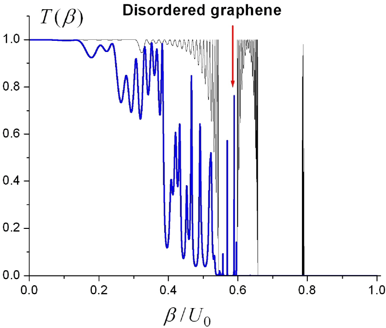
Figure 6: (color online) Transmission coefficient $T(\beta)$ for periodic (thin black line) and disordered (bold blue line) graphene. The range of the variation of the potentials, $\Delta u_{0}=0.1U_{0}$; $\varepsilon=0$.

One can see that a relatively weak disorder has drastically changed the transmission spectrum: all features of the spectrum of the underlying periodic structure has been washed out, and a rather dense (quasi-)discrete angular spectrum has appeared with the corresponding wave functions localized at random points inside the sample (disorder-induced resonances). Figure 7 shows the spatial distribution of the square modulus of the amplitude of a resonant wave function (intensity distribution inside the sample).

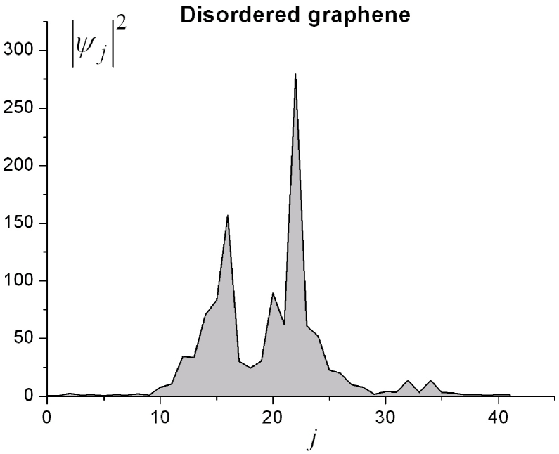
Figure 7: Spatial distribution of the wave function localized inside the sample for $\beta$ marked by a red arrow in Fig. 6.

For a fixed $\varepsilon$, $T(\beta)$, shown in Fig. 6, has the same form as $T(\varepsilon)$ for a fixed $\beta$, shown in Fig. 8. Both consist of randomly distributed resonances (one in the $\beta$ domain and another versus energy) typical for 1D Anderson localization of electrons and light. However, there is one fundamental difference from the usual Anderson localization: in the vicinity of normal incidence, the transmission spectrum of graphene is continuous with extended wave functions, and the transmission coefficient is finite ($T=1$ at $\theta=0)$. It is this range of angles that provides the finite minimal conductivity, which is proportional to the integral of $T(\theta)$ over all angles $\theta$.

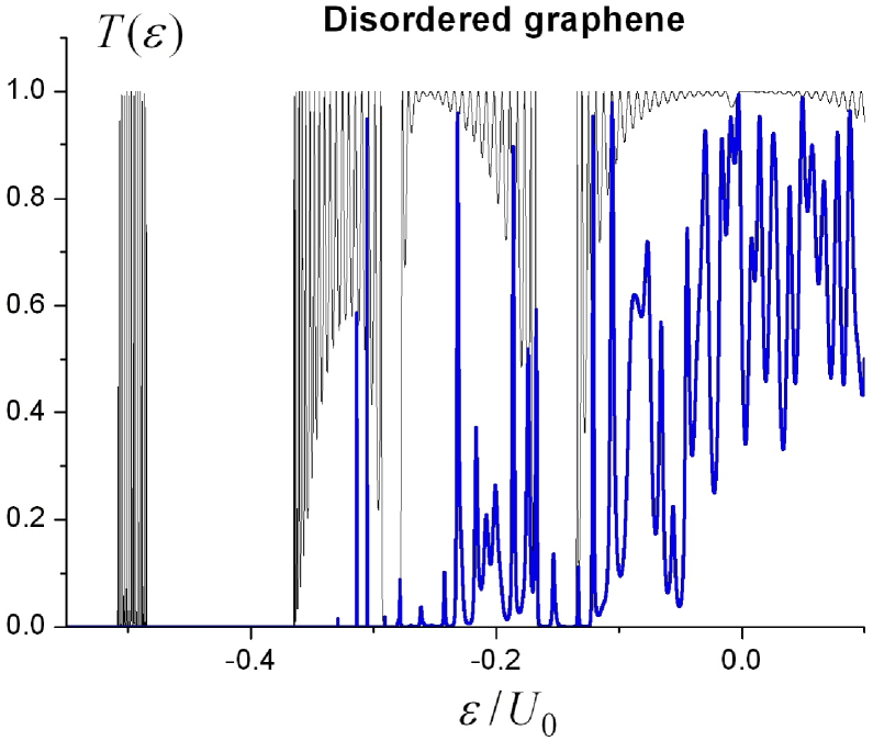
Figure 8: (color online) Transmission coefficient as a function of the energy $\varepsilon$, $T(\varepsilon)$, for periodic (thin black line) and disordered (bold blue line) graphene. $\Delta u_{0}=0.1U_{0}$, $\beta=0.3U_{0}$.

The mean transmission coefficient, $\langle T(\beta)\rangle$, for different strengths of disorder (different $\Delta u_{0}$) is plotted in Fig. 9. As expected, the increase of disorder reduces the transmission and narrows down the angular width of the transmission spectrum $\Delta\beta$. The zero (to within the resolution of the plots) values of $\langle T(\beta)\rangle$ at each curve correspond to the angles, which exceed the angle of total internal reflection.

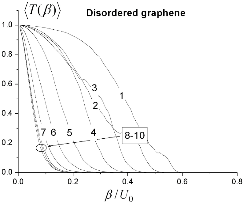
Figure 9: Mean transmission coefficient $\left\langle T(\beta)\right\rangle$ for disordered graphene. The curve (1) corresponds to $\Delta u_{0}/U_{0}=0.1$, the curve (2) corresponds to $\Delta u_{0}/U_{0}=0.2$, etc. Curves (8), (9), and (10), for which $\Delta u_{0}/U_{0}=0.8$, 0.9, and 1.0 are practically indiscernible.

IV.2 Case (ii): $\varepsilon\leq u_{0}(j)=\mathrm{const}$

In this case, the results are more intriguing Titov-1 ; San-Jose (although encountered in usual electron and optical random systems Fr-enhancement ). In this case, the transmission of the unperturbed system is exponentially small (tunneling) and gets enhanced by the fluctuation of the potential (Fig. 10).

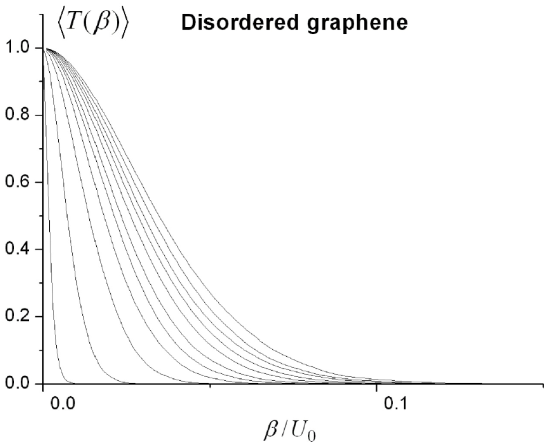
Figure 10: Mean transmission coefficient $\left\langle T(\beta)\right\rangle$ for disordered graphene for different values of the parameter $\Delta u_{0}/U_{0}$, which increases from zero (narrowest curve) to 1.0 (widest curve). Here, $\Delta u_{0}/U_{0}$ increases by 0.1 from left to right.

This is quite natural because the transmission of each $j$-th segment is proportional to $\exp[-\delta_{0}(\varepsilon\pm\Delta u_{j})]$ and (despite of the fact that $\langle\Delta u_{j}\rangle=0$) the mean value $\left\langle\exp[-\delta_{0}(\varepsilon\pm\Delta u_{j})]\right\rangle>\exp(-\delta_{0}\varepsilon)$, due to the asymmetry of the exponential function. Note that another type of disorder, linked to graphene layer edges, leads to the same result: the disorder improves the transmission Rozhkov , compared to the ordered graphene case.

IV.3 Case (iii): $|\Delta u_{j}|<|u_{0}(j)|$ and $u_{0}(j)=\pm U_{0}$

The behavior of the charge carriers in the graphene system of type (iii) is most unusual. It is characteristic of two-dimensional Fermions and have no analogies in electron and light transport. Shown in Fig. 11 by the bold blue line is the transmission spectrum at $\varepsilon=0$ of a graphene sample containing 40 layers of equal thicknesses $\delta_{j}=\delta_{0}$ and alternating random potential. One can see that, compared to the underlying periodic configuration (thin black line), the disorder: obliterates the transmission peaks located near $\beta_{m}$ with $m\neq 1$ [see Eq. (13)]; makes much wider the transparency zone near $\beta=0$; and gives rise to a new narrow peak in the transmission coefficient, associated with wave localization in the random potential. In contrast to the peaks in the periodic structure, the wave function of this disorder-induced resonance is exponentially localized.

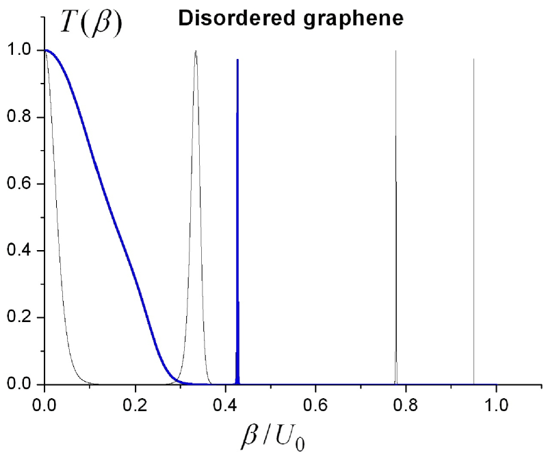
Figure 11: (color online) Transmission coefficient $T(\beta)$ for periodic (thin black line) and random (bold blue line) symmetric potential with $\Delta u_{j}\in(-0.1,0.1)$.

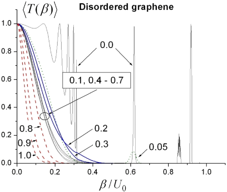
Figure 12: (color online) Mean transmission coefficient $\left\langle T(\beta)\right\rangle$ for disordered graphene. Arrows with numbers mark the strength of the disorder, $\Delta u_{0}/U_{0}$.

For this case (iii), the average transmission coefficient as a function of $\beta$ is presented in Fig. 12. In contrast to the case (i), the transmission in (iii) is extremely sensitive to fluctuations of the applied potential: in Fig. 12 the relative fluctuations $\Delta u_{0}/u_{0}=0.05$ reduce the angular width of the transmission spectrum more than four times (see also Fig. 13).

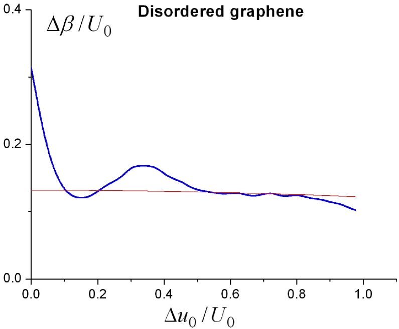
Figure 13: (color online) Half-width $\Delta\beta$ of the angular spectrum for a (iii) structure. Red thin line corresponds to the half-width $\Delta\beta$ given by Eq. (19).

That high sensitivity makes such a system a good candidate for use in electronic circuits capable of tuning the direction of charge flow. Another striking property is that after this abrupt drop in the transmission, it (i.e., the transmission) becomes practically independent of the strength of disorder in a relatively large range, as shown in Fig. 13.

The propagation of light in analogous L-R and R-R disordered dielectric structures demonstrates completely different behavior. As the degree of disorder (variations $\Delta n_{j}$ of the refractive indexes $n_{j})$ grows, the averaged angular spectra quickly reach their asymptotic “rectangular” shape: a constant transmission in the region where all interfaces between layers are transparent followed by an abrupt decrease in transmission in the region of $\beta$ where the total internal reflection appears (see Fig. 14b,c). The frequency dependences of the transmission coefficient and localization length have been studied in Ref. Asatryan, .

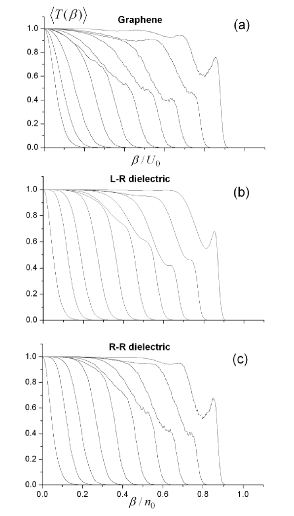
Figure 14: Mean transmission coefficient $\left\langle T(\beta)\right\rangle$ for: (a) disordered type (ii) graphene structure; (b) disordered L-R dielectric structure; (c) disordered R-R dielectric structure. Different curves correspond to the different values of the strength of the disorder $\Delta u_{0}/U_{0}$ in (a), $\delta n/n_{0}$ in (b) and (c), which increases from right to left from 0.1 to 1.0 with a step of 0.1.

V Analytical study

The features presented above can be explained, both qualitatively and quantitatively, in the framework of a rather simple theoretical approach. It can be shown matrices that in the short-wavelength limit, $k\delta\gg 1,$ the mean amplitude transmission coefficient, $\left\langle T^{(N)}\right\rangle$, of a sample built of $N$ layers, is approximately equal to

$$\left\langle T^{(N)}\right\rangle\simeq{\prod}_{j=1}^{N}\left\langle|t_{j,j+1}|^{2}\right\rangle,$$ (14)

where $t_{j,j+1}$ are statistically independent complex transmission coefficients of the boundaries between the $j$-th and $(j+1)$-th layers, and

$$|t_{j,j+1}|^{2}={\frac{2\cos^{2}\theta_{j+1}}{1+\cos(\theta_{j}-\theta_{j+1})},}$$ (15)

At small $\theta\ll 1$, equation (15) becomes

$$\left|t_{j,j+1}\right|^{2}\simeq 1-{\frac{3}{4}}\theta_{j+1}^{2}+{\frac{1}{4}}\theta_{j}^{2}-{\frac{1}{2}}\theta_{j}\theta_{j+1},$$ (16)

$$\theta_{j}=\arctan\left[{\frac{\beta}{\sqrt{(u_{j}-\varepsilon)^{2}-\beta^{2}}}}\right]\simeq{\frac{\beta}{|u_{j}-\varepsilon|}},$$

and from Eqs. (14) and (16) it follows that

$$\left\langle T^{(N)}\right\rangle\simeq\left[1-{\frac{1}{2}}\langle\theta^{2}\rangle-{\frac{1}{2}}\langle\theta\rangle^{2}\right]^{N}.$$ (17)

In an initially periodic array of alternating p-n and n-p junctions, $u_{j}=-u_{j+1}=U_{0},$ at $\varepsilon=0$ [structure (iii)], Eq. (17) yields

$$\left\langle T^{(N)}(\beta)\right\rangle\simeq 1-{\frac{1}{2}}{\frac{\beta^{2}}{(\Delta\beta)^{2}}},$$ (18)

where

$$\Delta\beta={\frac{U_{0}}{\sqrt{N}}}\left[{\frac{\ln 2}{1+\langle\delta u\rangle^{2}/2U_{0}^{2}}}\right]^{1/2}$$ (19)

is the half-width of the angular spectrum, defined as the value of $\beta$ where $\langle T^{(N)}(\beta)\rangle=1/2$. Equations (18), (19) fit well the numerical results presented in Figs. 12, 13. In particular, they describe the numerically observed quadratic dependence on $\beta$ and surprisingly weak dependence of the mean transmission on the strength of the disorder.

In a disordered graphene superlattice consisting only of n-n and p-p junctions [structure (ii)], the mean transmission coefficient $\left\langle T^{(N)}\right\rangle$ at $\langle\delta u^{2}\rangle/U_{0}^{2}\ll 1$ is given by

$$\left\langle T^{(N)}\right\rangle\simeq\left[1-{\frac{1}{2}}\langle\theta^{2}\rangle+{\frac{1}{2}}\langle\theta\rangle^{2}\right]^{N}\simeq\left[1-{\frac{1}{2}}{\frac{\beta^{2}}{U_{0}^{2}}}{\frac{\langle\delta u^{2}\rangle}{U_{0}^{2}}}\right]^{N}.$$ (20)

In this case, it is easy to see that the half-width of the angular spectrum strongly depends on the strength of the fluctuations and decreases with increasing $\langle\delta u^{2}\rangle/U_{0}^{2}$, as can be seen in Fig. 14a and in the relation:

$$\Delta\beta={\frac{U_{0}}{\sqrt{N}}}\left[{\frac{2\ln 2U_{0}^{2}}{\langle\delta u\rangle^{2}}}\right]^{1/2}.$$ (21)

Note, that in the cases (i) and (iii), the transmittance spectrum has parabolic shape for small angles of incidence, $\left\langle T^{(N)}(\beta)\right\rangle\simeq 1-\beta^{2}/\Delta\beta^{2}$, and the spectrum half-width $\Delta\beta$ decreases as $1/\sqrt{N}$ when the number $N$ of layers (the sample length $L$) increases. The same spectrum property for case (ii) has been predicted in Ref. San-Jose, .

In contrast to the charge transport in disordered graphene superlattices described above, the propagation of light in randomly layered dielectrics is similar (at $\theta\ll 1$) for L-R and RR arrays of layers with equal impedances (there are the analogs of p-n and p-p junctions, respectively). This follows from the fact that in both cases the small-angle asymptotics of the mean transmission coefficient through a boundary between layers are identical and at $\theta\ll 1$ have an universal form (compare with Eqs. 17, 18):

$$\left\langle\left|t_{j,j+1}\right|^{2}\right\rangle\simeq 1-\frac{1}{2}\left\langle\theta_{j+1}^{2}\right\rangle+\frac{1}{2}\left\langle\theta_{j}^{2}\right\rangle,$$

which yeilds

$$\left\langle T^{(N)}\right\rangle\simeq 1-O\left(\theta^{4}\right).$$ (22)

As in periodic systems, the difference in the transmission spectra of disordered graphene and dielectric samples [compare Eqs. (14), (20), and (22)] is a consequence of the above mentioned absence of imaginary part in the transfer matrix $\hat{\mathcal{M}}$, Eq. (9). Examples of the numerically calculated (with no approximations) angular spectra of the transmission of light are shown in Fig. 14b,c.

VI Geometrical disorder

In Section IV, we studied spatially-periodic layered graphene structures, in which the values of the applied potential in each layer were statistically independent random numbers. Further numerical calculations show that the main features of the transport and localization of charge in disordered graphene superlatices are rather universal, i.e., independent of the type of disorder. When instead of the amplitude of the potential, the size of each layer is fluctuating,

$$\Delta u_{j}=0,\hskip 8.53581pt\delta_{j}=\delta+\Delta_{j}$$

all results are similar, at least qualitatively. In Fig. 15, the angular dependences of the mean transmission coefficient, $\left\langle T(\beta)\right\rangle$, are plotted for different strengths of the geometrical disorder (different values of $\Delta/\delta$) in the case when $u_{j}<\varepsilon$ and assuming that $\Delta_{j}$ are independent random and homogeneously distributed in the interval $(-\Delta,\Delta)$. As it is in the corresponding case (i) of Section IV (Fig. 9), small disorder destroys the band structure of the underlaying periodic system, and with $\Delta/\delta$ increasing $\left\langle T(\beta)\right\rangle$ takes, in the vicinity of the normal incidence (small $\beta)$, a parabolic form, which remains unchanged when increasing disorder. When $\varepsilon=0$ and $u_{j}$ is a periodic set of numbers with alternating signs (an array of random p-n junctions corresponding to the case (iii) of Section IV), the shape of $\left\langle T(\beta)\right\rangle$ is also parabolic with the half-width similar to that shown in Fig. 13.

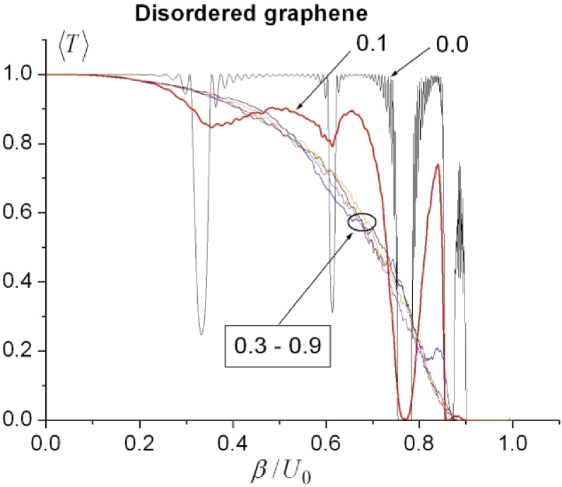
Figure 15: (color online) Mean transmission coefficient $\left\langle T(\beta)\right\rangle$ for graphene with geometrical disorder (section VI). Arrows with numbers mark the strength of disorder, $\Delta/\delta$.

VII Conclusions

We have studied the transport and localization of charge carriers in graphene superlattices produced by applying periodic and disordered potentials that depend on one coordinate. Simultaneously, the optical properties of analogue dielectric structures composed of traditional (right-handed, RH) dielectric and left-handed (LH) metamaterial layers was considered and compared with the charge transport in graphene. It was shown that in the Kronig-Penny-type periodic structures, a sort of total internal reflection can occur. In the case of a non-symmetric periodic array of alternating p-n and n-p junctions, along with the conduction bands and band gaps in the angular domain, there are also a discrete set of directions, in which the structures are resonantly transparent. In symmetric ($u_{1}=-u_{2}$, $\varepsilon=0$, and $\delta_{1}=\delta_{2}$) systems, the conduction zones disappear, and the angular spectrum of the transmission coefficient represents a discrete set of resonances, similar to the resonances in the symmetric ($n_{1}=-n_{2}$, $\delta_{1}=\delta_{2}$, and $Z_{1}\neq Z_{2}$) periodic alternating RH-LH dielectric structures. These features make the direction of the charge flux easily tunable by changing the applied voltage. The numerical experiments have shown that relatively weak disorder can drastically change the transmission properties of the underlaying periodic configurations. In the direction orthogonal to the layers created by a 1D random potential, the eigenstates are extended for all energies and a minimal conductivity remains non-zero, no matter how strong the disorder is. Away from the normal incidence, 1D random graphene systems manifest all features of disorder-induced strong localization. There exist a discrete random set of angles (or a discrete random set of energies for each given angle) for which the corresponding wave functions are exponentially localized. Depending on the type of the unperturbed system, the disorder could either suppress or enhance the transmission. The transmission of a graphene system built of alternating p-n and n-p junctions has anomalously narrow angular spectrum; is extremely sensitive to fluctuations of the applied potential; and, in some range of directions, it is practically independent of the amplitude of fluctuations of the potential. Our numerical results fit well the analytically calculated short wavelength asymptotics of the mean values of the corresponding transfer matrices. The main features of the charge transport in graphene subject to a disordered potential have been compared with those of the propagation of light in inhomogeneous dielectric media. This comparison has enabled better understanding of both physical processes.

References

- (1) M.I. Katsnelson and K.S Novoselov, Solid State Commun. 143, 3 (2007).
- (2) A.K. Geim and K.S. Novoselov, Nature Mat. 6, 183 (2007).
- (3) C-H. Parc, L. Yang, Y-W. Son, M. Cohen, and S. Louie, Nature Phys. 4, 213 (2008).
- (4) K.S. Novoselov, A.K. Geim, S.V. Morozov, D. Jiang, M.I. Katsnelson, I.V. Grigorieva, S.V. Dubonos, and A.A. Firsov, Nature (London) 438, 197 (2005).
- (5) A.H. Castro Neto, F. Guinea, N.M.R. Peres, K.S. Novoselov, and A.K. Geim, Rev. Mod. Phys. (in press), (2008); arXiv:cond-mat/0709.1163.
- (6) M.I. Katsnelson, K.S. Novoselov, and A.K. Geim, Nature Phys. 2, 620 (2006).
- (7) O. Klein, Z.Phys. 53, 157 (1929).
- (8) V.V. Cheianov, V. Fal’ko, and B.L. Altshuler, Science 315, 1252 (2007).
- (9) V.G. Veselago , Sov. Phys. Uspekhi. 10, 509 (1968) [Usp. Fiz. Nauk 92, 517 (1967)].
- (10) J.B. Pendry, Phys. Rev. Lett. 85, 3966 (2000).
- (11) N.M.R. Peres, F. Guinea, and A.H. Castro Neto, Phys. Rev. B 73, 125411 (2006).
- (12) J. Tworzydło, B. Trauzettel, M. Titov, A. Rycerz, and C.W.J. Beenakker, Phys. Rev. Lett. 96, 246802 (2006).
- (13) M. Titov, Europhys. Lett. 79, 17004 (2007).
- (14) P. San-Jose, E. Prada, and D.S. Golubev, Phys. Rev. B 76, 195445 (2007).
- (15) A.V. Rozhkov, S. Savel’ev, and F. Nori, arXiv:cond-mat/0808.1636.
- (16) F. Guinea, M.I. Katsnelson, and M.A.H. Vozmediano, Phys. Rev. B 77, 075422 (2008).
- (17) E. Rossi, S. Adam, and S.D. Sarma, arXiv:cond-mat/0809.1425.
- (18) Y. Zhang, Y.-W. Tan, H.L. Stormer, and P. Kim, Nature (London) 438, 201 (2005).
- (19) X-Z. Yan, C.S. Ting, Phys. Rev. Lett. 101, 126801 (2008).
- (20) For comparison of different definitions of localization and relevant terminology see math-loc .
- (21) C. de Oliveira, R. Prado, J. of Math. Phys. 46, 072105 (2005).
- (22) J.C. Slonczewski and P.R. Weiss, Phys. Rev. 109, 272 (1958).
- (23) G.W. Semenoff, Phys. Rev. Lett. 53, 2449 (1984).
- (24) V. Freilikher, B. Liansky, I. Yurkevich, A. Maradudin, and A. McGurn, Phys. Rev. E 51, 6301 (1995).
- (25) D. Dragoman and M. Dragoman, Quantum-classical analogies, Springer, Berlin, (2004).
- (26) P. Darancet, V. Olevano, and D. Mayou, arXiv:cond-mat/080.3553.
- (27) S. Tamura and F. Nori, Phys. Rev. B 41, 7941 (1990).
- (28) N. Nishiguchi, S. Tamura, and F. Nori, Phys. Rev. B 48, 2515 (1993).
- (29) N. Nishiguchi, S. Tamura, and F. Nori, Phys. Rev. B 48, 14426 (1993).
- (30) M. Born and E. Wolf, Principles of Optics, Cambridge University Press, Cambridge, UK, (1999).
- (31) M. Barbier, F. Peeters, P. Vasilopoulos, and M. Pereira, Jr, Phys. Rev. B 77, 115446 (2008).
- (32) C-H Park, L. Yang, Y-W Son, M. Cohen, and S. Louie, Phys. Rev. Lett. 101, 126804 (2008).
- (33) T.G. Pedersen, C. Flindt, J. Pedersen, N.A. Mortensen, A.-P. Jauho, and K. Pedersen, Phys. Rev. Lett. 100, 136804 (2008).
- (34) M. Diem, T. Koschny, and C. Soukoulis, arXiv:optics/0807.3351.
- (35) L. Wu, S. He, and L. Chen, Opt. Express 11, 1283 (1983).
- (36) L. Wu, S. He, and L. Shen, Phys. Rev. B 67, 235103 (2003).
- (37) R. Dragila, B. Luther-Davies, and S. Vukovic, Phys. Rev. Lett. 55, 1117 (1985).
- (38) J.M. Pereira, Jr., V. Mlinar, and F.M. Peeters, Phys. Rev. B 74, 045424 (2006).
- (39) V.A. Yampol’skii, S. Savel’ev, and F. Nori, New J. Phys. 10, 053024 (2008).
- (40) K. Nomura, M. Koshino, and S. Ryu, Phys. Rev. Lett. 99, 146806 (2007).
- (41) V. Freilikher, M. Pustilnik, and I. Yurkevich, Phys. Rev. B 53, 7413 (1996).
- (42) A. A. Asatryan, L.C. Botten, M.A. Byrne, V.D. Freilikher, S.A. Gredeskul, I.V. Shadrivov, R.C. McPhedran, and Y.S. Kivshar, Phys. Rev. Lett. 99, 193902 (2007).