Rare B decays with moving NRQCD and improved staggered quarks

$\>{}^{a}$, Eike H. Mรผllerb, Lew Khomskiia, Alistair Hartb, Ronald R. Horgana, Matthew Wingatea

aDAMTP, University of Cambridge, Wilberforce Road, Cambridge CB3 0WA, UK
bSUPA, School of Physics and Astronomy, University of Edinburgh, Edinburgh EH9 3JZ, UK

E-mail
Abstract:

We calculate form factors relevant for rare $B$ decays using moving-NRQCD for the $b$ quark and the AsqTad action for the light quarks. Moving NRQCD allows us to work directly with the physical $b$ quark mass and go to higher recoil momentum compared to standard NRQCD. Here, we show first results for the matrix elements and the operator matching coefficients. Some difficulties and possible ways of improvement are discussed.

1 Introduction

Decays of $B$ mesons via the flavour-changing-neutral-current transition bโ†’sโ†’๐‘๐‘ b\rightarrow s are particularly sensitive to possible new-physics contributions and provide tests of the CKM mechanism at the loop level. Measurements of exclusive modes like $B\rightarrow K^{*}\gamma$ have reached a good accuracy, and call for precise theoretical predictions. These are more difficult than for tree-level decays such as $B\rightarrow\pi l\nu$, since a large set of effective electroweak operators contributes and long-distance or spectator effects can be important. Nevertheless, the computation of hadronic form factors in lattice QCD is highly desirable and complements continuum approaches.

Matrix element Form factor Relevant decay(s)
$\langle P|\bar{q}\gamma^{\mu}b|B\rangle$ $f_{+},f_{0}$ $\left\{\begin{array}[]{l}B\to\pi\ell\nu\\ B\to K\ell^{+}\ell^{-}\end{array}\right.$
$\langle P|\bar{q}\sigma^{\mu\nu}q_{\nu}b|B\rangle$ $f_{T}$ ย ย ย ย ย Bโ†’Kโ€‹โ„“+โ€‹โ„“โˆ’โ†’๐ต๐พsuperscriptโ„“superscriptโ„“B\to K\ell^{+}\ell^{-}
$\begin{array}[]{c}\langle V|\bar{q}\gamma^{\mu}b|B\rangle\\ \langle V|\bar{q}\gamma^{\mu}\gamma^{5}b|B\rangle\end{array}$ $\begin{array}[]{c}V\\ A_{0},A_{1},A_{2}\end{array}$ $\left\{\begin{array}[]{l}B\to(\rho/\omega)\ell\nu\\ B\to K^{*}\ell^{+}\ell^{-}\end{array}\right.$
$\begin{array}[]{c}\langle V|\bar{q}\sigma^{\mu\nu}q_{\nu}b|B\rangle\\ \langle V|\bar{q}\sigma^{\mu\nu}\gamma^{5}q_{\nu}b|B\rangle\end{array}$ $\begin{array}[]{c}T_{1}\\ T_{2},T_{3}\end{array}$ $\left\{\begin{array}[]{l}B\to K^{*}\gamma\\ B\to K^{*}\ell^{+}\ell^{-}\end{array}\right.$
Table 1: Form factors for semileptonic and radiative $B$ decays.

We are currently working on the calculation of the form factors listed in Tableย 1. The combination of NRQCD and improved staggered actions for heavy-light mesons has already proven very successful in the calculation of form factors [1]. In order to extend the kinematic range to high recoil (lower $q^{2}$), we now use a moving-NRQCD (mNRQCD) action for the heavy quark. A brief discussion of our strategy can be found in [2], and a new detailed account of mNRQCD will be given in [3]. Here, we report on the progress in the computation of matrix elements and operator matching coefficients achieved so far.

2 Lattice methods

The matrix element $\langle F(p^{\prime})|J|B(p)\rangle$, where $F$ denotes the final pseudoscalar ($P$) or vector ($V$) meson and $J$ is the relevant current in the effective electroweak operator (see Tableย 1), can be extracted from the combination of the Euclidean 3-point correlator

CFโ€‹Jโ€‹Bโ€‹(๐ค(๐ช),๐ค(๐ฉ),x0,y0,z0)=โˆ‘๐ฒโˆ‘๐ณโŸจฮฆFโ€‹(x)โ€‹J(lat)โ€‹(y)โ€‹ฮฆBโ€ โ€‹(z)โŸฉโ€‹eโˆ’iโ€‹๐ฉโ€ฒโ‹…๐ฑโ€‹eโˆ’iโ€‹๐ค(๐ช)โ‹…๐ฒโ€‹eiโ€‹๐ค(๐ฉ)โ‹…๐ณsubscript๐ถ๐น๐ฝ๐ตsubscript๐ค๐ชsubscript๐ค๐ฉsubscript๐‘ฅ0subscript๐‘ฆ0subscript๐‘ง0subscript๐ฒsubscript๐ณdelimited-โŸจโŸฉsubscriptฮฆ๐น๐‘ฅsuperscript๐ฝlat๐‘ฆsuperscriptsubscriptฮฆ๐ตโ€ ๐‘งsuperscript๐‘’โ‹…๐‘–superscript๐ฉโ€ฒ๐ฑsuperscript๐‘’โ‹…๐‘–subscript๐ค๐ช๐ฒsuperscript๐‘’โ‹…๐‘–subscript๐ค๐ฉ๐ณC_{FJB}(\mathbf{k}_{(\mathbf{q})},\>\mathbf{k}_{(\mathbf{p})},\>x_{0},\>y_{0},\>z_{0})=\sum_{\mathbf{y}}\sum_{\mathbf{z}}\left\langle\Phi_{F}(x)\>J^{(\mathrm{lat})}(y)\>\Phi_{B}^{\dagger}(z)\right\rangle e^{-i\mathbf{p^{\prime}}\cdot\mathbf{x}}e^{-i\mathbf{k}_{(\mathbf{q})}\cdot\mathbf{y}}e^{i\mathbf{k}_{(\mathbf{p})}\cdot\mathbf{z}} (1)

with the two-point functions

$\displaystyle C_{BB}(\mathbf{k}_{(\mathbf{p})},\>x_{0},\>y_{0})$ $\displaystyle=$ โˆ‘๐ฑโŸจฮฆBโ€‹(x)โ€‹ฮฆBโ€ โ€‹(y)โŸฉโ€‹eโˆ’iโ€‹๐ค(๐ฉ)โ‹…(๐ฑโˆ’๐ฒ),subscript๐ฑdelimited-โŸจโŸฉsubscriptฮฆ๐ต๐‘ฅsuperscriptsubscriptฮฆ๐ตโ€ ๐‘ฆsuperscript๐‘’โ‹…๐‘–subscript๐ค๐ฉ๐ฑ๐ฒ\displaystyle\sum_{\mathbf{x}}\left\langle\Phi_{B}(x)\>\Phi_{B}^{\dagger}(y)\right\rangle e^{-i\mathbf{k}_{(\mathbf{p})}\cdot(\mathbf{x}-\mathbf{y})}, (2)
$\displaystyle C_{FF}(\mathbf{p^{\prime}},\>x_{0},\>y_{0})$ $\displaystyle=$ โˆ‘๐ฑโŸจฮฆFโ€‹(x)โ€‹ฮฆFโ€ โ€‹(y)โŸฉโ€‹eโˆ’iโ€‹๐ฉโ€ฒโ‹…(๐ฑโˆ’๐ฒ).subscript๐ฑdelimited-โŸจโŸฉsubscriptฮฆ๐น๐‘ฅsuperscriptsubscriptฮฆ๐นโ€ ๐‘ฆsuperscript๐‘’โ‹…๐‘–superscript๐ฉโ€ฒ๐ฑ๐ฒ\displaystyle\sum_{\mathbf{x}}\left\langle\Phi_{F}(x)\>\Phi_{F}^{\dagger}(y)\right\rangle e^{-i\mathbf{p^{\prime}}\cdot(\mathbf{x}-\mathbf{y})}. (3)

Here, $\Phi_{B}$ and $\Phi_{F}$ are suitable interpolating fields for the initial and final meson, and $J^{(\mathrm{lat})}$ is a lattice version of the current, obtained by operator matching (see section 3). For the light quarks, we convert from 1-component staggered to 4-component naive fields [4]. Due to the use of mNRQCD for the $b$ quark, the physical momenta $\mathbf{p}$ and $\mathbf{q}$ are related to the lattice momenta $\mathbf{k}_{(\mathbf{p})}$ and $\mathbf{k}_{(\mathbf{q})}$ by

$\displaystyle\mathbf{p}$ $\displaystyle=$ $\displaystyle\mathbf{k}_{(\mathbf{p})}+Z_{p}\>\gamma\>m_{b}\mathbf{v},$
$\displaystyle\mathbf{q}$ $\displaystyle=$ $\displaystyle\mathbf{k}_{(\mathbf{q})}+Z_{p}\>\gamma\>m_{b}\mathbf{v}$ (4)

where $Z_{p}\approx 1$ is the renormalisation of the external momentum, $\gamma=1/\sqrt{1-\mathbf{v}^{2}}$ and $\mathbf{v}$ is the boost velocity. One has $\mathbf{p^{\prime}}=\mathbf{p}-\mathbf{q}=\mathbf{k}_{(\mathbf{p})}-\mathbf{k}_{(\mathbf{q})}$. The physical energy $p_{0}=E_{B}$ of the $B$ meson is also shifted,

$\displaystyle E_{B}(\mathbf{p})=E_{\mathbf{v}}(\mathbf{k}_{(\mathbf{p})})+\Delta_{\mathbf{v}}$ (5)

where $E_{\mathbf{v}}(\mathbf{k}_{(\mathbf{p})})$ is the unphysical energy obtained from the fit to the correlator and $\Delta_{\mathbf{v}}$ is the velocity-dependent energy shift. Writing $t=|x_{0}-y_{0}|$ and $T=|x_{0}-z_{0}|$, the correlators are fitted by

$\displaystyle C_{FJB}(\mathbf{k}_{(\mathbf{q})},\>\mathbf{k}_{(\mathbf{p})},\>t,\>T)$ $\displaystyle\rightarrow$ $\displaystyle\sum_{k=0}^{K-1}\>\>\sum_{l=0}^{L-1}A_{kl}^{(FJB)}(-1)^{k\>t}(-1)^{l(T-t)}e^{-E^{\prime}_{k}t}e^{-E_{l}(T-t)},$ (6)
$\displaystyle C_{BB}(\mathbf{k}_{(\mathbf{p})},\>t)$ $\displaystyle\rightarrow$ $\displaystyle\sum_{l=0}^{L-1}A_{l}^{(BB)}(-1)^{l(t+1)}e^{-E_{l}t},$ (7)
$\displaystyle C_{FF}(\mathbf{p^{\prime}},\>t)$ $\displaystyle\rightarrow$ $\displaystyle 16\sum_{k=0}^{K-1}A_{k}^{(FF)}(-1)^{k(t+1)}e^{-E^{\prime}_{k}t}$ (8)

or equivalent parametrisations. Every other exponential comes with an oscillating pre-factor, as required by the use of naive quarks [4]. The correlator $C_{FF}$ receives an extra factor of 16 due to the trace over a $16\times 16$ taste matrix, while the heavy-light correlators $C_{BB}$ and $C_{FJB}$ receive contributions from only one taste [4]. The ground-state fit parameters are related to the matrix elements as follows:

$\displaystyle A_{00}^{(FJB)}$ $\displaystyle=$ {ZV2โ€‹EVโ€‹ZB2โ€‹EBโ€‹โˆ‘sฮตjโ€‹(pโ€ฒ,s)โ€‹โŸจVโ€‹(pโ€ฒ,ฮตโ€‹(pโ€ฒ,s))|J|Bโ€‹(p)โŸฉ,F=V,ZP2โ€‹EPโ€‹ZB2โ€‹EBโ€‹โŸจPโ€‹(pโ€ฒ)|J|Bโ€‹(p)โŸฉ,F=Pcasessubscript๐‘๐‘‰2subscript๐ธ๐‘‰subscript๐‘๐ต2subscript๐ธ๐ตsubscript๐‘ subscript๐œ€๐‘—superscript๐‘โ€ฒ๐‘ quantum-operator-product๐‘‰superscript๐‘โ€ฒ๐œ€superscript๐‘โ€ฒ๐‘ ๐ฝ๐ต๐‘๐น๐‘‰subscript๐‘๐‘ƒ2subscript๐ธ๐‘ƒsubscript๐‘๐ต2subscript๐ธ๐ตquantum-operator-product๐‘ƒsuperscript๐‘โ€ฒ๐ฝ๐ต๐‘๐น๐‘ƒ\displaystyle\left\{\begin{array}[]{ll}\displaystyle\frac{\sqrt{Z_{V}}}{2E_{V}}\frac{\sqrt{Z_{B}}}{2E_{B}}\sum_{s}\varepsilon_{j}(p^{\prime},s)\>\langle V\left(p^{\prime},\varepsilon(p^{\prime},s)\right)|\>J\>|B(p)\rangle,&F=V,\\ \displaystyle\frac{\sqrt{Z_{P}}}{2E_{P}}\frac{\sqrt{Z_{B}}}{2E_{B}}\>\langle P\left(p^{\prime}\right)|\>J\>|B(p)\rangle,&F=P\end{array}\right. (11)
$\displaystyle A_{0}^{(BB)}$ $\displaystyle=$ $\displaystyle\frac{Z_{B}}{2E_{B}}$ (12)
$\displaystyle A_{0}^{(FF)}$ $\displaystyle=$ {โˆ‘sZV2โ€‹EVโ€‹ฮตjโˆ—โ€‹(pโ€ฒ,s)โ€‹ฮตjโ€‹(pโ€ฒ,s),F=V,ZP2โ€‹EP,F=P.casessubscript๐‘ subscript๐‘๐‘‰2subscript๐ธ๐‘‰subscriptsuperscript๐œ€๐‘—superscript๐‘โ€ฒ๐‘ subscript๐œ€๐‘—superscript๐‘โ€ฒ๐‘ ๐น๐‘‰subscript๐‘๐‘ƒ2subscript๐ธ๐‘ƒ๐น๐‘ƒ\displaystyle\left\{\begin{array}[]{ll}\displaystyle\sum_{s}\frac{Z_{V}}{2E_{V}}\>\varepsilon^{*}_{j}(p^{\prime},s)\varepsilon_{j}(p^{\prime},s),&F=V,\\ \displaystyle\frac{Z_{P}}{2E_{P}},&F=P.\end{array}\right. (15)

The amplitudes $\sqrt{Z_{B}}$, $\sqrt{Z_{P}}$ and $\sqrt{Z_{V}}$ in (11) depend on the form of the interpolating fields $\Phi_{B}$, $\Phi_{P}$ and $\Phi_{V}$ and can be extracted from (12) and (15).

3 Operator matching

The continuum currents $J$ must be replaced by lattice currents $J^{(\mathrm{lat})}$ containing suitable matching coefficients to correct for the different ultraviolet behaviour of QCD and lattice mNRQCD. As only the high-energetic modes with $E\gtrsim m_{b}$ differ in the theories and ฮฑsโ€‹(mb)โ‰ช1much-less-thansubscript๐›ผ๐‘ subscript๐‘š๐‘1\alpha_{s}(m_{b})\ll 1, matching coefficients can be computed perturbatively.

We use tadpole-improved 1-loop lattice perturbation theory. The Feynman rules are generated automatically [5] and diagrams are evaluated using the Monte Carlo integrator VEGAS.

The first step is the computation of a set of heavy-quark renormalisation parameters from the self-energy diagrams: the zero-point energy $E_{0}$, the wavefunction renormalisation $Z_{\psi}$, the renormalisation of the mass $Z_{m}$ and the renormalisation of the boost velocity $Z_{v}$ [6, 3]. Results for the full improved $\mathcal{O}(\Lambda_{QCD}^{2}/m_{b}^{2})$ lattice mNRQCD action will be presented in [3].

Once these parameters are known, one can proceed with the calculation of matching coefficients. For the (axial-)vector currents, these have been computed in the static limit (i.e. neglecting $\mathcal{O}(\Lambda_{QCD}/m_{b})$ corrections in $J^{(\mathrm{lat})}$), and the calculation including the $\mathcal{O}(\Lambda_{QCD}/m_{b})$ corrections is underway [7]. In the following, we focus on the tensor current, which, in the continuum, is given by111For the matching calculation, we treat the light quark as massless; in this limit the matching coefficients for the last two operators in Tab.ย 1 are equal due to chiral symmetry.

$\displaystyle J_{7}^{\mu\nu}$ $\displaystyle=$ $\displaystyle\frac{e}{16\pi^{2}}m_{b}\;\overline{q}\sigma^{\mu\nu}b\qquad\mathrm{with}\quad\sigma^{\mu\nu}=\frac{i}{2}[\gamma^{\mu},\gamma^{\nu}].$ (16)

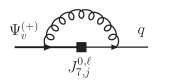
We work in the static limit. At this order in the heavy-quark expansion there are two operators with different Dirac structure in lattice mNRQCD. For the $\mu=0$ components one has

$\displaystyle J_{7,1}^{0\ell}$ $\displaystyle=$ $\displaystyle-\frac{e}{16\pi^{2}}m_{b}\sqrt{\frac{\scriptstyle 1+\gamma}{\scriptstyle 2\gamma}}\left(\overline{q}\sigma_{0\ell}\Psi_{v}^{(+)}\right),$
$\displaystyle J_{7,2}^{0\ell}$ $\displaystyle=$ $\displaystyle i\frac{e}{16\pi^{2}}m_{b}\>v\sqrt{\frac{\scriptstyle\gamma}{\scriptstyle 2(1+\gamma)}}\left(\overline{q}\sigma_{0\ell}\vec{\hat{v}}\cdot\vec{\gamma}\gamma_{0}\Psi_{v}^{(+)}\right)$ (17)

where $\Psi_{v}^{(+)}$ denotes the mNRQCD field with the antiquark components set to zero. On the lattice, these operators mix under renormalisation; the one-particle irreducible vertex correction that contributes in the static limit is shown in Fig. 2.

Refer to caption

Figure 1: Vertex correction diagram.

Refer to caption

Figure 2: Matching coefficients for the tensor current. The subtraction point is $\mu=1/a$.

Writing $J_{7,\pm}^{0\ell}=J_{7,1}^{0\ell}\pm J_{7,2}^{0\ell}$, we obtain the lattice operator

$\displaystyle J_{7}^{(\mathrm{lat})0\ell}$ $\displaystyle=$ (1+ฮฑsโ€‹c10โ€‹โ„“)โ€‹J7,10โ€‹โ„“+(1+ฮฑsโ€‹c20โ€‹โ„“)โ€‹J7,20โ€‹โ„“1subscript๐›ผ๐‘ superscriptsubscript๐‘10โ„“superscriptsubscript๐ฝ710โ„“1subscript๐›ผ๐‘ superscriptsubscript๐‘20โ„“superscriptsubscript๐ฝ720โ„“\displaystyle(1+\alpha_{s}c_{1}^{0\ell})J_{7,1}^{0\ell}+(1+\alpha_{s}c_{2}^{0\ell})J_{7,2}^{0\ell} (18)
$\displaystyle=$ (1+ฮฑsโ€‹c+0โ€‹โ„“)โ€‹J7,+0โ€‹โ„“+ฮฑsโ€‹cโˆ’0โ€‹โ„“โ€‹J7,โˆ’0โ€‹โ„“.1subscript๐›ผ๐‘ superscriptsubscript๐‘0โ„“superscriptsubscript๐ฝ70โ„“subscript๐›ผ๐‘ superscriptsubscript๐‘0โ„“superscriptsubscript๐ฝ70โ„“\displaystyle(1+\alpha_{s}c_{+}^{0\ell})J_{7,+}^{0\ell}+\alpha_{s}c_{-}^{0\ell}J_{7,-}^{0\ell}.

The matching coefficients $c_{\pm}^{0\ell}$ must be adjusted such that $J_{7}^{(\mathrm{lat})0\ell}$ has the same one-loop matrix elements as the tensor operator in the continuum theory. They depend on the lattice spacing and contain a logarithmic ultraviolet divergence as the tensor operator is not conserved.
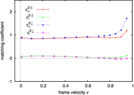
Results using an improved $\mathcal{O}(\Lambda_{QCD}/m_{b})$ mNRQCD action at $am=2.8$, $n=2$, the AsqTad action for the light quark and the Lรผscher-Weisz gluon action are shown in Fig. 2. The matching coefficient of the operator $J_{7,-}^{0\ell}$, which only arises at 1-loop level, is strongly suppressed and the dependence on the frame velocity is found to be small for all matching coefficients.

4 Details of the numerical calculations and first results

In our first computations of the 3-point functions (1) we used the local interpolating fields $\Phi_{B}(z)=\bar{q}^{\prime}(z)\gamma_{5}b(z)$ and $\Phi_{F}(x)=\bar{q}^{\prime}(x)\Gamma_{F}q(x)$ with $\Gamma_{P}=\gamma_{5},\>\Gamma_{V}=\gamma_{1,2,3}$. As in standard NRQCD, the heavy-quark Green function $G_{b}(y,z)$ can be obtained by solving an initial value problem. Let us consider the case $x_{0}>y_{0}>z_{0}$. Schematically, as initial value at $z_{0}$ we use the propagator of the light valence quark, $\gamma_{5}\>G_{q^{\prime}}(z,x)$, and then evolve the heavy-quark Green function up to the time slice $y_{0}$ where we perform the contraction with the various gamma matrices and the other light-quark propagator Gqโ€‹(x,y)=ฮณ5โ€‹Gqโ€ โ€‹(y,x)โ€‹ฮณ5subscript๐บ๐‘ž๐‘ฅ๐‘ฆsubscript๐›พ5superscriptsubscript๐บ๐‘žโ€ ๐‘ฆ๐‘ฅsubscript๐›พ5G_{q}(x,y)=\gamma_{5}G_{q}^{\dagger}(y,x)\gamma_{5}. This method only requires light-quark propagators with a fixed origin $x$, and, since the current is inserted only in the final contraction, allows the efficient simultaneous computation of arbitrary currents.

These initial calculations were done on 400 MILC gauge configurations of size $20^{3}\times 64$ with 2+1 flavours of light quarks, at $\beta=6.76$ and $a^{-1}\approx 1.6$ GeV. The light sea quark masses were $am_{u}=am_{d}=0.007$, aโ€‹ms=0.05๐‘Žsubscript๐‘š๐‘ 0.05am_{s}=0.05 and the light valence quark masses $am_{u}=am_{d}=0.007$, aโ€‹ms=0.04๐‘Žsubscript๐‘š๐‘ 0.04am_{s}=0.04 (we used the AsqTad action). On each configuration, we took four different origins $x$, and additionally averaged with the time-reversed process.

Even though we have implemented the full $\mathcal{O}(\Lambda_{QCD}^{2}/m_{b}^{2})$ mNRQCD action, we only used an $\mathcal{O}(\Lambda_{QCD}/m_{b})$ mNRQCD action here to save computer time. This is sufficiently accurate since we only considered currents in the static limit here. The heavy-quark mass was set to $am_{b}=2.8$ and the stability parameter was $n=2$. All lattice momenta and the boost velocity were always pointing in 1-direction. In this case, 21 combinations of operators/indices and final-state polarisations give non-zero contributions, and all the form factors listed in Table 1 can be extracted from them.

We performed Bayesian multi-exponential fits in the two variables $T$ and $t$. Gaussian priors for the ground state energies were taken from fit results of the corresponding two-point functions, with widths equal to the error from the fit result. The mNRQCD energy shift $\Delta_{\mathbf{v}}$ (see eq. (5)) was determined non-perturbatively from heavy-heavy meson dispersion relations (for those, the full mNRQCD action accurate to $v_{nr}^{4}$ in heavy-heavy power counting was used). A bootstrap analysis was used to determine the form factors and their statistical errors.

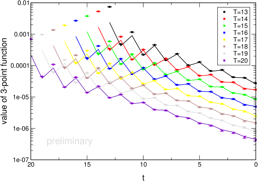
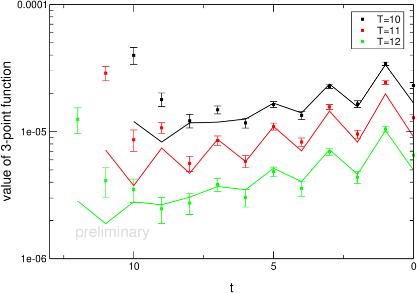
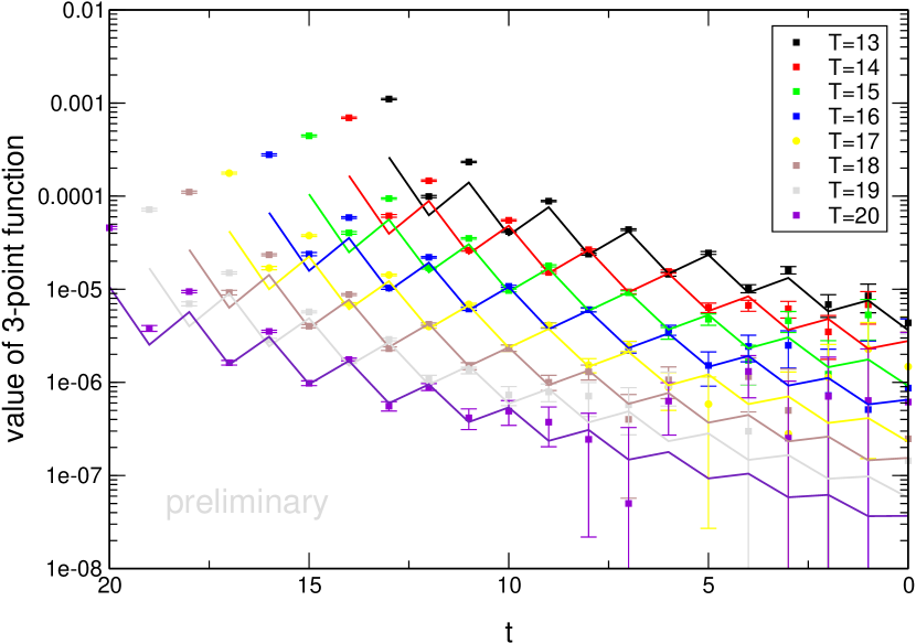
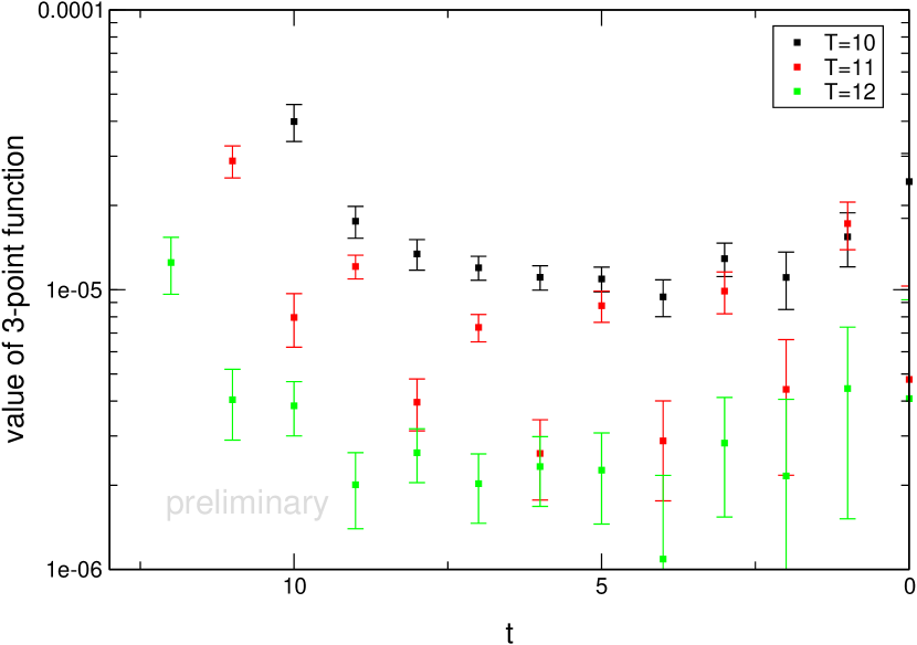
To give some examples, plots of the 3-point correlators โŸจฮฆKโ€‹sยฏโ€‹ฮณ0โ€‹bโ€‹ฮฆBโ€ โŸฉdelimited-โŸจโŸฉsubscriptฮฆ๐พยฏ๐‘ subscript๐›พ0๐‘superscriptsubscriptฮฆ๐ตโ€ \langle\>\>\Phi_{K}\>\>\>\bar{s}\gamma_{0}b\>\>\>\Phi_{B}^{\dagger}\>\>\rangle and โŸจฮฆKโˆ—โ€‹sยฏโ€‹ฯƒ13โ€‹bโ€‹ฮฆBโ€ โŸฉdelimited-โŸจโŸฉsubscriptฮฆsuperscript๐พยฏ๐‘ subscript๐œŽ13๐‘superscriptsubscriptฮฆ๐ตโ€ \langle\>\>\Phi_{K^{*}}\>\>\>\bar{s}\sigma_{13}b\>\>\>\Phi_{B}^{\dagger}\>\>\rangle at the largest $q^{2}$ (with $\mathbf{v}=0$) are shown in Fig. 4 and 4. The results for the tensor current in combination with the vector meson final state are much noisier. As expected, the statistical errors are seen to grow further when the recoil momentum is increased. In Fig. 6 and 6 we show the corresponding correlators at $\mathbf{v}=(0.4,0,0)$ and $\mathbf{k}_{(\mathbf{p})}=\frac{2\pi}{L}(1,0,0)$, $\mathbf{k}_{(\mathbf{q})}=\frac{2\pi}{L}(2,0,0)$. Note that for the fits shown here, 4..6 timeslices from the source/sink were skipped, so that $K=2$, $L=4$ (for the vector final state) or $K=1$, $L=3$ (for the pseudoscalar final state) was sufficient in (6). The results can probably be improved by extending the fitting range and using more exponentials.

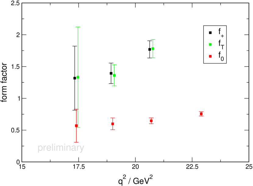
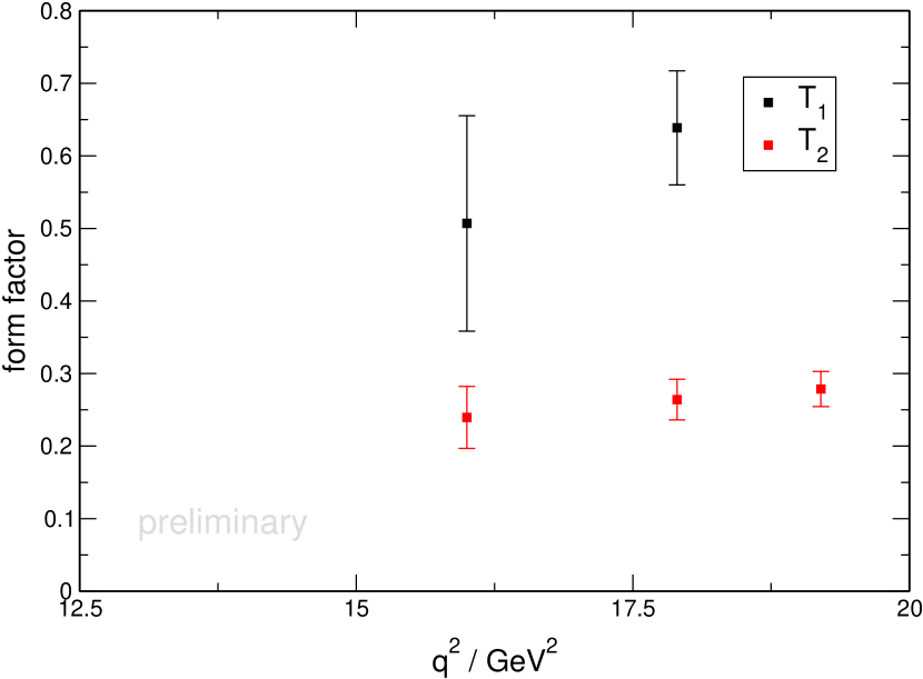
Finally, in Fig. 8 and 8 we show some first results for the form factors $f_{0}$, $f_{+}$, $f_{T}$ and $T_{1}$, $T_{2}$. Note that the momentum of the meson in the final state ($K$ or $K^{*}$) was exclusively set to the very small values $\mathbf{p^{\prime}}=0$ or $\mathbf{p^{\prime}}=\frac{2\pi}{L}(-1,0,0)$. This is made possible by the use of moving NRQCD.

Refer to caption

Figure 3: Three-point correlator โŸจฮฆKโ€‹sยฏโ€‹ฮณ0โ€‹bโ€‹ฮฆBโ€ โŸฉdelimited-โŸจโŸฉsubscriptฮฆ๐พยฏ๐‘ subscript๐›พ0๐‘superscriptsubscriptฮฆ๐ตโ€ \langle\>\>\Phi_{K}\>\>\>\bar{s}\gamma_{0}b\>\>\>\Phi_{B}^{\dagger}\>\>\rangle at $\mathbf{k}_{(\mathbf{p})}=0$, $\mathbf{k}_{(\mathbf{q})}=0$, $\mathbf{v}=0$. The fitting range is $T=14\>...\>18$ and $t=6\>...\>(T-5)$.

Refer to caption

Figure 4: Three-point correlator โŸจฮฆKโˆ—โ€‹sยฏโ€‹ฯƒ13โ€‹bโ€‹ฮฆBโ€ โŸฉdelimited-โŸจโŸฉsubscriptฮฆsuperscript๐พยฏ๐‘ subscript๐œŽ13๐‘superscriptsubscriptฮฆ๐ตโ€ \langle\>\>\Phi_{K^{*}}\>\>\>\bar{s}\sigma_{13}b\>\>\>\Phi_{B}^{\dagger}\>\>\rangleat $\mathbf{k}_{(\mathbf{p})}=0$, $\mathbf{k}_{(\mathbf{q})}=\frac{2\pi}{L}(1,0,0)$, $\mathbf{v}=0$. The fitting range is $T=8\>...\>20$ and $t=4\>...\>(T-4)$ (not all data shown for legibility).

Refer to caption

Figure 5: Three-point correlator โŸจฮฆKโ€‹sยฏโ€‹ฮณ0โ€‹bโ€‹ฮฆBโ€ โŸฉdelimited-โŸจโŸฉsubscriptฮฆ๐พยฏ๐‘ subscript๐›พ0๐‘superscriptsubscriptฮฆ๐ตโ€ \langle\>\>\Phi_{K}\>\>\>\bar{s}\gamma_{0}b\>\>\>\Phi_{B}^{\dagger}\>\>\rangle at $\mathbf{k}_{(\mathbf{p})}=\frac{2\pi}{L}(1,0,0)$, $\mathbf{k}_{(\mathbf{q})}=\frac{2\pi}{L}(2,0,0)$, $\mathbf{v}=(0.4,0,0)$. The fitting range is $T=14\>...\>18$ and $t=6\>...\>(T-5)$.

Refer to caption

Figure 6: Three-point correlator โŸจฮฆKโˆ—โ€‹sยฏโ€‹ฯƒ13โ€‹bโ€‹ฮฆBโ€ โŸฉdelimited-โŸจโŸฉsubscriptฮฆsuperscript๐พยฏ๐‘ subscript๐œŽ13๐‘superscriptsubscriptฮฆ๐ตโ€ \langle\>\>\Phi_{K^{*}}\>\>\>\bar{s}\sigma_{13}b\>\>\>\Phi_{B}^{\dagger}\>\>\rangleat $\mathbf{k}_{(\mathbf{p})}=\frac{2\pi}{L}(1,0,0)$, $\mathbf{k}_{(\mathbf{q})}=\frac{2\pi}{L}(2,0,0)$, $\mathbf{v}=(0.4,0,0)$. No reasonable fit was achieved yet.

Refer to caption

Figure 7: The form factors $f_{+}$, $f_{0}$, $f_{T}$ (points for $f_{+}$ and $f_{T}$ are offset horizontally for legibility). The points at lowest $q^{2}$ have $\mathbf{v}=(0.4,0,0)$, $\mathbf{k}_{(\mathbf{p})}=\frac{2\pi}{L}(1,0,0)$, $\mathbf{k}_{(\mathbf{q})}=\frac{2\pi}{L}(2,0,0)$.

Refer to caption

Figure 8: The form factors $T_{1}$, $T_{2}$. The points at lowest $q^{2}$ have $\mathbf{v}=(0.2,0,0)$, $\mathbf{k}_{(\mathbf{p})}=\frac{2\pi}{L}(1,0,0)$, $\mathbf{k}_{(\mathbf{q})}=\frac{2\pi}{L}(2,0,0)$.

5 Conclusions

Using moving-NRQCD and AsqTad actions, we have calculated matching coefficients for the heavy-light axial-, vector- and tensor currents in the static limit using 1-loop lattice perturbation theory, and performed first computations of form factors for rare $B$ decays. While moving NRQCD significantly reduces discretisation errors at low $q^{2}$, our initial results suffer from large statistical errors, overshadowing the advantages of the method. However, statistical errors do not constitute a fundamental obstacle and can be reduced further. The first step will be to extend the fitting range and include more exponentials. Then, we plan to work with random-wall sources, which were shown to provide considerable improvement for semileptonic decays at high recoil momentum [8]. We will also use smeared interpolating fields to reduce contributions from excited states, thereby improving the fits. Furthermore, note that our initial computations were done with lattice momenta pointing in the 1-direction only. Off-axial momenta and boost velocities will also allow lower values for $q^{2}$, for example by using the final meson momentum $\mathbf{p^{\prime}}=\frac{2\pi}{L}(-1,-1,\>\>0)$.

Once statistical errors are under control, we will study the dependence on the lattice spacing and the light quark masses. We also plan to include $\mathcal{O}(\Lambda_{QCD}/m_{b})$ operators in the matching calculations.

Acknowledgements

This work has made use of the resources provided by the Edinburgh Compute and Data Facility (which is partially supported by the eDIKT initiative), the Fermilab Lattice Gauge Theory Computational Facility and the Cambridge High Performance Computing Facility. We thank the MILC collaboration for making their gauge configurations publicly available.

References

  • [1] E.ย Dalgic, A.ย Gray, M.ย Wingate, C.ย T.ย H.ย Davies, G.ย P.ย Lepage and J.ย Shigemitsu, Phys.ย Rev.ย  D 73, 074502 (2006) [Erratum-ibid.ย  D 75, 119906 (2007)] [arXiv:hep-lat/0601021]
  • [2] S.ย Meinel, R.ย Horgan, L.ย Khomskii, L.ย C.ย Storoni and M.ย Wingate, PoS LAT2007, 377 (2007) [arXiv:0710.3101 [hep-lat]].
  • [3] [HPQCD and UKQCD Collaborations], Moving NRQCD for High Recoil Form Factors in Heavy Quark Physics, in preparation.
  • [4] M.ย Wingate, J.ย Shigemitsu, C.ย T.ย H.ย Davies, G.ย P.ย Lepage and H.ย D.ย Trottier, Phys.ย Rev.ย  D 67, 054505 (2003) [arXiv:hep-lat/0211014].
  • [5] A.ย Hart, G.ย M.ย von Hippel, R.ย R.ย Horgan and L.ย C.ย Storoni, J.ย Comput.ย Phys.ย  209, 340 (2005) [arXiv:hep-lat/0411026].
  • [6] A.ย Dougall, C.ย T.ย H.ย Davies, K.ย M.ย Foley and G.ย P.ย Lepage [HPQCD Collaboration and UKQCD Collaboration], Nucl.ย Phys.ย Proc.ย Suppl.ย  140, 431 (2005) [arXiv:hep-lat/0409088].
  • [7] L.ย Khomskii, Perturbation Theory for Quarks and Currents in Moving NRQCD on a Lattice, PhD thesis, in preparation.
  • [8] C.ย T.ย H.ย Davies, E.ย Follana, K.ย Y.ย Wong, G.ย P.ย Lepage and J.ย Shigemitsu, PoS LAT2007, 378 (2007) [arXiv:0710.0741 [hep-lat]].