From time series to complex networks: the visibility graph
Published in PNAS, vol. 105, no. 13 (2008) 4972-4975.

Resumen

In this work we present a simple and fast computational method, the visibility algorithm, that converts a time series into a graph. The constructed graph inherits several properties of the series in its structure. Thereby, periodic series convert into regular graphs, and random series do so into random graphs. Moreover, fractal series convert into scale-free networks, enhancing the fact that power law degree distributions are related to fractality, something highly discussed recently. Some remarkable examples and analytical tools are outlined in order to test the method’s reliability. Many different measures, recently developed in the complex network theory, could by means of this new approach characterize time series from a new point of view.

In this letter we introduce a new tool in time series analysis: the visibility graph. This algorithm maps a time series into a network. The main idea is to study into which extend the techniques and focus of graph theory are useful as a way to characterize time series. As will be shown below, this network inherits several properties of the time series, and its study reveals non trivial information about the series itself.

For illustrative purposes, in figure (1) we present a scheme of the visibility algorithm. In the upper zone we plot the first twenty values of a periodic series using vertical bars (the data values are displayed above the plot). Considering this as a landscape, we link every bar (every point of the time series) with all those that can be seen from the top of the considered one (gray lines), obtaining the associated graph (shown in the lower part of the figure). In this graph, every node corresponds, in the same order, to a series data, and two nodes are connected if there exists visibility between the corresponding data, that is to say, if there is a straight line that connects the series data, provided that this “visibility line” does not intersect any intermediate data height.

More formally, we can establish the following visibility criterium: two arbitrary data $(t_{a},y_{a})$ and $(t_{b},y_{b})$ will have visibility, and consequently will become two connected nodes of the associated graph, if any other data $(t_{c},y_{c})$ placed between them fulfills:

$$y_{c}<y_{b}+(y_{a}-y_{b})\frac{t_{b}-t_{c}}{t_{b}-t_{a}}\mathchar 46\relax$$ (1)

We can easily check that by means of the present algorithm, the associated graph extracted from a time series is always:
(i) connected: each node sees at least its nearest neighbors (left and right).
(ii) undirected: the way the algorithm is built up, there is no direction defined in the links.
(iii) invariant under affine transformations of the series data: the visibility criterium is invariant under rescaling of both horizontal and vertical axis, as well as under horizontal and vertical translations (see figure 2).
In a recent work [1], Zhang $\&$ Small (ZS) introduced another mapping between time series and complex networks. While the philosophy is similar to this work (to encode the time series in a graph in order to characterize the series using graph theory), there exist fundamental differences between both methods, mainly in what refers to the range of applicability (ZS only focus on pseudoperiodic time series, associating each series cycle to a node and defining links between nodes via temporal correlation measures, while the visibility graph can be applied to every kind of time series) and the graph connectedness (in ZS the giant component is assured only ad hoc, meanwhile the visibility graph is always connected by definition).

The key question is to know whether the associated graph inherits some structure of the time series, and consequently if the process which generated the time series may be characterized using graph theory. In a first step we will consider periodic series. As a matter of fact, the example plotted in figure 1 is nothing but a periodic series with period $4$. The associated visibility graph is regular, as long as it is constructed by periodic repetition of a pattern. The degree distribution of this graph is formed by a finite number of peaks related to the series period, much in the vein of the Fourier Power Spectrum of a time series. Generically speaking, all periodic time series are mapped into regular graphs, the discrete degree distribution being the fingerprint of the time series periods. In the case of periodic time series, its regularity seems therefore to be conserved or inherited structurally in the graph by means of the visibility map.

As an opposite to periodic series, in a second step we will tackle a series $R(t)$ of $10^{6}$ data extracted from an uniform distribution in $[0,1]$. Although one would expect in a first moment a Poisson degree distribution in this case (as for uncorrelated random graphs [2]), a random time series has indeed some correlation, since it is an ordered set. In fact, let $k_{t}$ be the connectivity of the node associated to the data $t$. If $k_{t}$ is large (related to the fact that the data has a large value and that consequently it has large visibility), one would expect that $k_{t+1}$ would be relatively small, since the time series is random and two consecutive data with a large value are not likely to occur. It is indeed due to these ’unlikely’ large values (the hubs) that the tail of the degree distribution deviates from the Poisson distribution. Two large values in the series data can be understood as two rare events in the random process. The time distribution of these events is indeed exponential [3, 4], therefore we should expect the tail of the degree distribution in this case to be exponential instead of Poissonian, as long as the form of this tail is related to the hub’s distribution.

In the left side of figure 3 we depict the first 250 values of $R(t)$. In the right side we plot the degree distribution $P(k)$ of its visibility graph. The tail of this distribution fits quite well an exponential distribution, as expected. Note at this point that time series extracted randomly from other distributions than uniform have also been addressed. In every case the algorithm captures the random nature of the series, and the particular shape of the degree distribution of the visibility graph is related to the particular random process [4].

Hitherto, ordered (periodic) series convert into regular graphs, and random series convert into exponential random graphs: order and disorder structure in the time series seem to be inherited in the topology of the visibility graph. Thus, the question arises: What kind of visibility graph is obtained from a fractal time series? This question is in itself interesting at the present time. Recently, the relationship between self-similar and scale-free networks [5, 10, 11, 12, 13] has been intensively discussed [6, 7, 8, 9]. While complex networks [10] usually exhibit the Small-World property [14] and cannot be consequently size-invariant, it has been recently shown [6] that applying fitted box-covering methods and renormalization procedures, some real networks actually exhibit self-similarity. So, whereas self-similarity seems to imply scale-freeness, the opposite is not true in general.

In order to explore these issues in more detail, the following two fractal series will be considered: the well-known Brownian motion $B(t)$ and the Conway series [15]. While the Brownian motion represents a well-known case of self-affinity (indeed, the following relation holds: $B(t)=a^{1/2}B(t/a)$), the Conway series $a(n)-n/2$ is the recursively generated fractal series from:

$$a(1)=a(2)=1$$

$$a(n)=a(a(n-1))+a(n-a(n-1));\ n>2\mathchar 46\relax$$

In figure 4 we have plotted the behavior of these series, the degree distribution $P(k)$ of their respective visibility graphs and their mean path length $L(N)$ as a function of the series length. First, both series have visibility graphs with degree distributions that correspond to power laws of the shape $P(k)\sim k^{-\alpha}$, where we get different exponents in each case: this result enhances the fact that in the context of the visibility algorithm, power law degree distributions (that is, scale free networks [10, 11, 12, 13]) arise naturally from fractal series. Moreover, this relation seems to be robust as long as the preceding examples show different kinds of fractality: while $B(t)$ stands for a stochastic self-affine fractal, the Conway series is a deterministic series recursively generated. On the other hand, while the Brownian visibility graph seems to evidence the Small-World effect (right top figure 4) as $L(N)\sim\log(N)$, the Conway series shows in turn a self-similar relation (right bottom figure 4) of the shape $L(N)\sim N^{\beta}$. This fact can be explained in terms of the so called hub repulsion phenomenon [8]: visibility graphs associated to stochastic fractals such as the Brownian motion or generic noise series do not evidence repulsion between hubs (in these series it is straightforward that the data with highest values would stand for the hubs, and these data would have visibility between each other), and consequently won’t be fractal networks following Song et al. [8]. On the other hand, the Conway series actually evidence hub repulsion: this series is concave-shaped and consequently the highest data won’t in any case stand for the hubs; the latter ones would be located much likely in the monotonic regions of the series, which are indeed hidden from each other (effective repulsion) across the series local maxima. The Conway visibility graph is thus fractal.
Since a fractal series is characterized by its Hurst exponent, we may argue that the visibility graph can actually distinguish different types of fractality, something that will be explored in detail in further work. Note at this point that some other fractal series have been also studied (Q series [16], Stern series [17], Thue-Morse series [18], etc) with similar results. Moreover, observe that if the series under study increases its length, the resulting visibility graph can be interpreted in terms of a model of network growth and may eventually shed light into the fractal network formation problem.

In order to cast light into the relation between fractal series and power law distributions, in the left part of figure 5 we present a deterministic fractal series generated by iteration of a simple pattern of three points. The series starts (step 0) with three points (A,B,C) of coordinates $(0,1)$, $(1,1/3)$ and $(2,1/3)$ respectively. In step p, we introduce $2^{p+1}$ new points with height $3^{-p-1}$ and distanced $3^{-p}$. The series form a self-similar set: applying an isotropic zoom of horizontal scale $3^{p}$ and vertical scale $3^{p}$ to the pattern of order p, we recover the original pattern.

Note that this time series is not data uniformly spaced as the previous examples. However its usefulness is set on the fact that it is simple enough to handle it analytically, that is to say, to find the degree distribution of its visibility graph. The main idea is to find a recurrence behavior in the way that a given node increases its connectivity when the fractal step (that is to say, the fractal size) is increased [19]. Then we calculate how many nodes (self-similar to it) appear in each step, and from both relations we come to a degree distribution for these kind of nodes.
First, from a quick visual exploration of left figure 5 one comes to the conclusion that nodes A and B have typically the same degree. In the other hand, the degree of node C can be decomposed in two terms, the left degree (due to visibility of nodes at the left of C) and right degree. The degree of A and B is the same as the right degree of C (statistically speaking, A and B increase their connectivity as the fractal size increases much in the way of the right part of C). Thereby, the degree of C provides the whole information of the system. We will quote $K_{r}(C,n)$ the right degree of node C in a n-step fractal (respectively, $K_{l}(C,n)$ stands for the left degree).
Applying the visibility criterium, one can geometrically find that

$$K_{r}(C,n)=\sum_{m=1}^{n}\frac{1}{m}\sum_{d|m}\mu(d)\cdot 2^{m/d},$$ (3)

where $\mu$ is the Moëbius function. Note that this summation agrees with the number of irreducible polynomials of degree at most $n$ over the Galois field GF(2) [20], something which deserves an in-depth investigation. This expression can be approximated by

$$K_{r}(C,n)\sim 2^{4n/5}\mathchar 46\relax$$ (4)

On the other hand, there is a recurrence in the left degree that reads

$$K_{l}(C,n)=2K_{l}(C,n-1)+1,$$ (5)

whose leading term is

$$K_{l}(C,n)\sim 2^{n}\mathchar 46\relax$$ (6)

The node $C$ will thus have a degree $K(C)=K_{r}(C,n)+K_{l}(C,n)$. In figure 5 (right) we plot the values of $K_{r}$ (circles) and $K_{l}$ (squares) as a function of the fractal size (the number of iterations $n$). Numerical values are plotted as the outer circles and squares, while the inner circles and squares come from plotting equations (3,5). Note that both formulas reproduce the numerical data. The straight lines correspond to the approximation equations (4) and (6). Now, in a generic step p, $2^{p}$ nodes which are self-similar to C appear (by construction). Those nodes will have a degree $K(C,n-p)=2^{\frac{4}{5}(n-p)}+2^{n-p}$ that, for large values of $n-p$, can be approximated to $K(C,n-p)\simeq 2^{n-p}$ . Defining $f(K)$ as the degree distribution, we get that $f\big{(}K(C,n-p)\big{)}=2^{p}$, and with the change of variable $u\equiv 2^{n-p}$, it is easy to come into:

$$f(u)\sim u^{-1},$$ (7)

that is, the degree distribution related to the C-nodes is a power law.
Although this simple example doesn’t provide a general explanation of why fractality is traduced into power law distributions, it may stand as a generic way of dealing with deterministic fractal series generated by iteration.

Once the visibility method has been presented, some remarks can be stated: note that typically two series that only differ by an affine transformation will have the same visibility graph; in this sense the algorithm absorbs the affine transformation. Furthermore, it is straightforward to see that that some information regarding the time series is inevitably lost in the mapping from the fact that the network structure is completely determined in the (binary) adjacency matrix. For instance, two periodic series with the same period as $T_{1}=\{\mathchar 46\relax\mathchar 46\relax,3,1,3,1,\mathchar 46\relax\mathchar 46\relax\}$ and $T_{2}=\{\mathchar 46\relax\mathchar 46\relax,3,2,3,2,\mathchar 46\relax\mathchar 46\relax\}$ would have the same visibility graph albeit being quantitatively different. While the spirit of the visibility graph is to focus on time series structural properties (periodicity, fractality, etc), the method can be trivially generalized using weighted networks (where the adjacency matrix isn’t binary and the weights determine the slope of the visibility line between two data) if we eventually need to quantitatively distinguish time series like $T_{1}$ and $T_{2}$ for instance.

While in this paper we have only tackled undirected graphs, note that one could also extract a directed graph (related to the temporal axis direction) in such a way that for a given node one should distinguish two different connectivities: an ingoing degree $k_{in}$, related to how many nodes see a given node $i$, and an outgoing degree $k_{out}$, that is the number nodes that node $i$ sees. In that situation, if the direct visibility graph extracted from a given time series is not invariant under time reversion (that is, if $P(k_{in})\neq P(k_{out})$), one could assert that the process that generated the series is not conservative. In a first approximation we have studied the undirected version and the directed one will be eventually addressed in further work.

There are some direct applications of the method that can be put forward. The relation between the exponent of the degree distributions and the Hurst exponent of the series will be addressed in further work. In particular, it turns out that the method presented here constitutes a reliable tool to estimate Hurst exponents, as far as a functional relation between the Hurst exponent of a fractal series and the degree distribution of its visibility graph holds [21]. Note that the estimation of Hurst exponents is an issue of major importance in data analysis that is yet to be completely solved (see for instance [22]). Fractional Brownian motions, a concept of great interest in a large variety of fields ranging from electronic devices to Biology, will also be considered in relation with the preceding point.
Moreover, the ability of the algorithm to detect not only the difference between random and chaotic series but also the spatial location of inverse bifurcations in chaotic dynamical systems is another fundamental issue that will also be at the core of further investigations [21]. Finally, the visibility graph characterizes non trivial time series and in that sense, the method may be relevant in specific problems of different garments, such as human behavior time series recently put forward [23].

In summary, a brand new algorithm that converts time series into graphs is presented. The structure of the time series is conserved in the graph topology: periodic series convert into regular graphs, random series into random graphs and fractal series into scale-free graphs. Such characterization goes beyond, since different graph topologies arise from apparently similar fractal series. In fact, the method captures the hub repulsion phenomenon associated to fractal networks [8] and thus distinguishes scale free visibility graphs evidencing Small-World effect from those showing scale invariance.
With the visibility algorithm a natural bridge between complex networks theory and time series analysis is now built.

We want to acknowledge the comments from the editor and two anonymous referees. The research was supported by grant FIS2006-08607 from the Spanish Ministry of Science.

Figura 1: Example of a time series ($20$ data) and the associated graph derived from the visibility algorithm. In the graph, every node corresponds, in the same order, to a series data. The visibility rays between the data define the links connecting nodes in the graph.

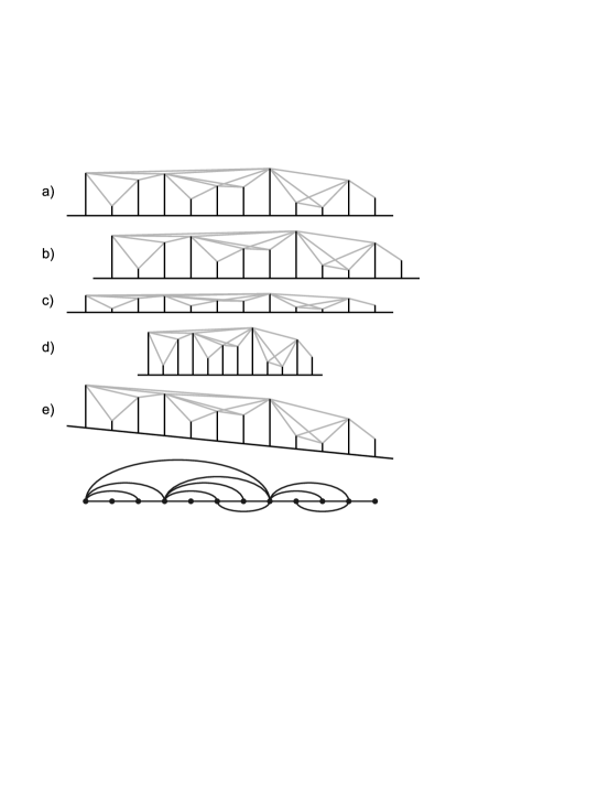
Figura 2: The visibility graph of a time series remains invariant under several transformation of the time series: a) original time series with visibility links b) translation of the data c) vertical rescaling d) horizontal rescaling e) addition of a linear trend to the data. As can be seen in the botom figure, in all these cases the visibility graph remains invariant.

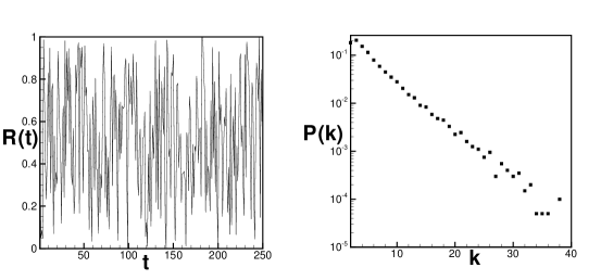
Figura 3: Left figure: First 250 values of $R(t)$, where $R$ is a random series of $10^{6}$ data extracted from U[0,1]. Right figure: degree distribution $P(k)$ of the visibility graph associated to $R(t)$ (plotted in semi-log). While the beginning of the curve approaches the result of a Poisson process, the tail is clearly exponential. This behavior is due to data with large values (rare events), which are the hubs.

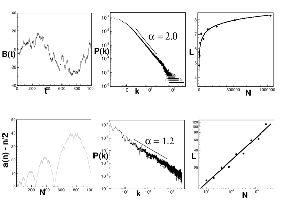
Figura 4: Upper part, from left to right: First 4000 data from a Brownian series of $10^{6}$ data. In the middle, the degree distribution of the visibility graph associated to the Brownian motion. This one is a power law $P(k)\sim k^{-\alpha}$ with $\alpha=2{,}00\pm 0{,}01$. In the right part of the figure we plot the mean path length of this network as a function of the network size N. The best fitting provides a logarithmic scaling $L(N)=1{,}21+0{,}51\log(N)$. This network shows Small-World effect in addition to be scale-free. Bottom part, from left to right: First $10^{5}$ data from a Conway series of $4\cdot 10^{6}$ data. In the middle, the degree distribution of the visibility graph associated to the Conway series. This one is a power law $P(k)\sim k^{-\alpha}$ with $\alpha=1{,}2\pm 0{,}1$. The mean path length as a function of the size N is depicted in the right part of the figure. The best fitting provides a power law scaling $L(N)=0{,}76N^{0{,}38}$. Then, this network is scale-invariant.

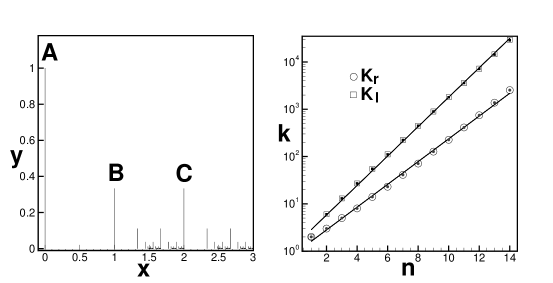
Figura 5: Left: Fractal series obtained by iteration of the original pattern (points A,B,C) with $p=10$ steps. Right: Values of $K_{r}$ (circles) and $K_{l}$ (squares) as a function of the fractal size, related to equations (3,5). Note that the plot is log-linear: the relation is thus exponential. The straight lines correspond to the approximations deduced in equations (4,6).

- [1] J. Zhang, M. Small, Phys. Rev. Lett. 96, 238701 (2006).
- [2] B. Bollobás, Modern Graph Theory, Springer-Verlag, New York Inc. (1998).
- [3] W. Feller, An Introduction to Probability Theory and its Applications, John Willey and Sons, Inc. (1971).
- [4] This feature will be adressed in further work.
- [5] A.L. Barabási, R. Albert, Science 286, 509 (1999).
- [6] C. Song, S. Havlin, H.A. Makse, Nature 433, 392 (2005).
- [7] K.I. Goh, G. Salvi, B. Kahng, D. Kim, Phys. Rev. Lett. 96 (2006).
- [8] C. Song, S. Havlin, H.A. Makse, Nat. Phys. 2,275 (2006).
- [9] J.S.Kim, K.I. Goh, G. Salvi, E. Oh, B. Kahng, D. Kim, Phys. Rev. E 75, 016110 (2007).
- [10] R. Albert, A.L. Barabási, Rev. Mod. Phys. 74 (2002).
- [11] M.E.J. Newman, SIAM Review 45 (2003) 167-256.
- [12] S. Dorogovtsev, J.F.F Mendes, Advances in Physics 51, 4 (2002).
- [13] S. Bocaletti, V. Latora, Y. Moreno, M. Chávez and D.U. Hwang, Phys. Reports 424 (2006) 175-308.
- [14] D.J. Watts and S.H. Strogatz, Nature 393, 440-442 (1998).
- [15] J. Conway, Some Crazy Sequences, Lecture at ATT Bell Labs (1988).
- [16] D. Hofstadter, Gödel, Escher, Bach, New York: Vintage Books, pp. 137-138 (1980).
- [17] M.A. Stern, J. Reine Angew. Math., 55, pp. 193-220 (1858).
- [18] M.R. Schroeder, Fractals, Chaos, and Power Laws, New York: W. H. Freeman (1991).
- [19] A.L. Barabási, E. Ravasz, and T. Vicsek, Physica A 299, 559-564 (2001).
- [20] K.H. Hicks, G.L. Mullen, and I. Sato, Distribution of irreducible polynomials over , in Finite Fields with Applications to Coding Theory, Cryptography and Related Areas (Oaxaca, 2001), 177-186, Springer, Berlin, 2002.
- [21] To be published.
- [22] T. Karagiannis, M. Molle and M. Faloutsos, Internet Computing, IEEE 8, 5 (2004).
- [23] A. Vázquez, J. Gama Oliveira, Z. Desz, K. Goh, I. Kondor and A.L. Barabási, Phys. Rev. E 73, 036127 (2006).