Density matrix renormalization group approach to two-fluid open many-fermion systems

Abstract

We have extended the density matrix renormalization group (DMRG) approach to two-fluid open many-fermion systems governed by complex-symmetric Hamiltonians. The applications are carried out for three- and four-nucleon (proton-neutron) systems within the Gamow Shell Model (GSM) in the complex-energy plane. We study necessary and sufficient conditions for the GSM+DMRG method to yield the correct ground state eigenvalue and discuss different truncation schemes within DMRG. The proposed approach will enable configuration interaction studies of weakly-bound and unbound strongly interacting complex systems which, because of a prohibitively large size of Fock space, cannot be treated by means of the direct diagonalization.

I Introduction

The theoretical description of weakly bound and unbound states in atomic nuclei requires a rigorous treatment of many-body correlations in the presence of scattering continuum and decay channels Jac_d ; Jac_o ; ppnp . Many-body states located close to the particle emission threshold display unusual properties such as, e.g., halo and Borromean structures, clusterization phenomena, and cusps in various observables resulting from the strong coupling to the continuum space. These peculiar features cannot be described in the standard shell model (SM) in which the single-particle (s.p.) basis is usually derived from an infinite well such as the harmonic oscillator potential. Indeed, resonance and scattering states, which play a decisive role in the structure of weakly bound/unbound states, are not properly treated within the standard SM formalism.

The solution of the configuration-interaction problem in the presence of continuum states has been recently advanced in the real-energy continuum SM Kar ; Rot ; Volya and in the complex-energy SM, the so-called Gamow Shell Model (GSM) Mic02a ; Bet02 ; Bet04 ; Mic06 ; Hag06 . In the GSM, the s.p. basis is given by the Berggren ensemble containing Gamow states and the non-resonant continuum of scattering states. The scattering states are distributed along a contour defined in the complex $k$-plane and, together with the Gamow states, form a complete set Berggren . In practice, the contour is discretized and the many-body basis is spanned by the Berggren ensemble. As in standard SM applications, the dimension of the many-body valence space increases dramatically with the number of valence nucleons and the size of the s.p. basis. Moreover, the use of the Berggren ensemble implies complex-symmetric matrices for the representation of the Hermitian Hamilton operator. Consequently, efficient numerical methods are needed to solve the many-body Schrödinger equation of GSM. The DMRG approach is ideally suited to optimize the size of the scattering space in the GSM problem as the properties of the non-resonant shells vary smoothly along the scattering contour.

The DMRG method was first introduced to overcome the limitations of the Wilson-type renormalization group to describe strongly correlated 1D lattice systems with short-range interactions dmrg1 (see recent reviews Rev1 ; Rev2 ; Rev3 ). More recently, by reformulating the DMRG in a s.p. basis, several applications to finite Fermi systems like molecules pap2 ; chan , superconducting grains pap3 ; delft , quantum dots pap4 ; weiss , atomic nuclei pap1 , and fractional quantum Hall systems Fei have been reported. While most of the DMRG studies were focused on equilibrium properties in strongly correlated closed quantum systems characterized by Hermitian density matrices, non-equilibrium systems involving non-Hermitian and non-symmetric density matrices can also be treated pap6 . Nuclear applications of DMRG in the context of the standard SM, both in the $M$-scheme and in the angular-momentum conserving $J$-scheme, have also been reported pap5 ; pitsan ; pitsan1 with mixed success. In the previous study Rot2 , we reported the first application of the DMRG method in the context of the GSM and showed that in this case the method provides a highly accurate description of broad resonances in the neutron-rich nuclei with few valence particles.

The present study is an extension of the previous work Rot2 to the case where both protons and neutrons are included in the valence space. Several significant improvements over Ref.  Rot2 have been made concerning the DMRG algorithm and numerical implementation. Our work is organized as follows. In Sec. II, we briefly recapitulate the GSM formalism and the generalized variational principle behind it. Section III describes the DMRG method in the $J$-scheme as applied to the open-system formalism of the GSM. Practical applications of the GSM+DMRG method are presented in Sec. IV. Illustrative calculations are carried out for ⁷Li (three-nucleon systems) and ⁸Li (four-nucleon systems). We study the impact of different starting conditions on the DMRG result and introduce two different truncation schemes in the DMRG procedure and discuss their virtues. The truncation schemes are compared with the GSM benchmark diagonalization results. The resulting efficient calculation scheme opens a window for extending calculations to systems beyond the current limits of direct diagonalization. The conclusions of our work are contained in Sec. V.

II The Gamow Shell Model

The s.p. basis used in the GSM formalism is generated by a finite depth potential. It forms a complete set of states in the sense of the Berggren completeness relation Berggren :

$$\sum_{n=b,d}|\tilde{u}_{n}\rangle\langle u_{n}|+\int_{L^{+}}|\tilde{u}_{k}\rangle\langle u_{k}|=1,$$ (1)

where the discrete sum includes s.p. bound (negative-energy) resonant states ($b$) and positive-energy decaying resonant states ($d$). These states are the poles of the corresponding one-body scattering matrix. The integration in Eq. (1) is performed along a contour $L^{+}$ defined in the complex $k$-plane that is located below the resonant states included in the basis (see Fig. 1). In general, different contours can be used for each $\ell,j$ partial wave.

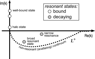
Figure 1: Illustration of the Berggren completeness relation (1) in the complex $k$-plane. The bound states are located on the positive imaginary axis. The weakly bound halo states lie close to the origin. The positive-energy resonant states are located in the fourth quadrant. Those with a small imaginary part can be interpreted as resonances. The complex-$k$ shells on the contour $L^{+}$ represent the non-resonant scattering continuum.

By discretizing continuum states on $L^{+}$ a finite s.p. basis is obtained. The many-body basis is obtained in the usual way by constructing product states (Slater determinants) from this discrete s.p. set. We assume in the following that the nucleus can be described as a system of $n_{\pi}$ protons and $n_{\nu}$ neutrons evolving around a closed core. Within this picture, the GSM Hamiltonian $\hat{H}$ reads:

$$\hat{H} = \sum_{i=1}^{n_{\pi}+n_{\nu}}\left[\frac{{\bf{{p_{i}}^{2}}}}{2\mu}+U_{i}\right]+\sum_{j>i=1}^{n_{\pi}+n_{\nu}}V_{ij},$$ (2)

where ${\bf{{p_{i}^{2}}}}/{2\mu}$ is the s.p. kinetic energy operator, $\mu$ is the reduced mass of the nucleon+core system, $U_{i}$ is the finite-depth, one-body potential, and $V_{ij}$ is the two-body residual interaction.

The GSM Hamiltonian (2) is complex symmetric. According to the complex variational principle moisey1 ; moisey , a complex analog to the usual variational principle for self-conjugated Hamiltonians, the Rayleigh quotient

$$E[\Phi]=\frac{\langle\Phi^{*}|\hat{H}|\Phi\rangle}{\langle\Phi^{*}|\Phi\rangle}$$ (3)

is stationary around any eigenstate $|\Phi_{0}\rangle$ of $\hat{H}$:

$$\hat{H}|\Phi_{0}\rangle=E[\Phi_{0}]|\Phi_{0}\rangle.$$ (4)

That is, at $|\Phi\rangle$=$|\Phi_{0}\rangle$ the variation of the functional $E[\Phi]$ is zero:

$$\delta_{\Phi}{E[\Phi]}_{\Phi=\Phi_{0}}=0.$$ (5)

It should be noted moisey1 ; moisey that the complex variational principle is a stationary principle rather than an upper or lower bound for either the real or imaginary part of the complex eigenvalue. However, it can be very useful when applied to the squared modulus of the complex eigenvalue moisey2 . Indeed,

$$\delta_{\Phi}{|E|^{2}}=\delta_{\Phi}{(E^{*}E)}=E^{*}\delta_{\Phi}{E}+E\delta_{\Phi}{E^{*}}=0$$ (6)

at $|\Phi\rangle$=$|\Phi_{0}\rangle$ because of analyticity of $E[\Phi]$.

III The Density Matrix Renormalization Group method for the Gamow Shell Model

Let us consider a nucleus with $n_{\pi}$ active protons and $n_{\nu}$ active neutrons and let us denote by $|J^{\pi}\rangle$ the eigenstate of $\hat{H}$ having angular momentum $J$ and parity $\pi$. As $|J^{\pi}\rangle$ is the many-body pole of the scattering matrix of $\hat{H}$, the contribution from scattering shells on $L^{+}$ to the many-body wave function is usually smaller than the contribution from the resonant orbits. Based on this observation, the following separation is usually performed Rot2 : the many-body states constructed from the s.p. poles form a subspace $A$ (the so-called ‘reference subspace’), and the remaining states containing contributions from non-resonant shells form a complement subspace $B$. As we shall discuss later in Sections IV.1 and IV.2, this intuitive definition of the reference subspace may be insufficient for describing certain classes of eigenstates. In such cases, states in $A$ have to be constructed both from the s.p. poles and selected scattering shells.

At the first stage of the GSM+DMRG method, called ’the warm-up phase’, the scattering shells are gradually added to the reference subspace to create the subspace $B$. This process is described in the next section.

III.1 Warm-up phase of GSM+DMRG

One begins by constructing all states $|k\rangle_{A}$ forming the reference subspace $A$. The set of those states shall be denoted as $\{k_{A}\}$. The many-body configurations in $A$ can be classified in different families $\{n;j_{A}^{\pi}\}$ according to their number of nucleons $n$, total angular momentum $j_{A}$, and parity $\pi$. In the following, we shall omit the parity label in the notation of a given family. States with a number of protons (neutrons) larger than $n_{\pi}$ ($n_{\nu}$) are not considered since they do not contribute to the many-body states in the composition of subspaces $A$ and $B$.

All possible matrix elements of suboperators of the two-body Hamiltonian (2) acting in $A$, expressed in the second quantization form, are calculated and stored:

$$\{O\} = \{a^{\dagger},(a^{\dagger}\,\widetilde{a})^{K},(a^{\dagger}a^{\dagger})^{K},((a^{\dagger}a^{\dagger})^{K}\widetilde{a})^{L},$$ (7)

$$(a^{\dagger}a^{\dagger})^{K}(\widetilde{a}\widetilde{a})^{K}\},$$

with $a^{\dagger}$ and $\widetilde{a}$ being the nucleon creation and annihilation operators in resonant shells. The GSM Hamiltonian is then diagonalized in the reference space to provide the zeroth-order approximation $|\Psi_{J}\rangle^{(0)}$ to $|J^{\pi}\rangle$. This vector, called ‘reference state’, plays an important role in the GSM+DMRG truncation algorithm.

In the next step, the subspace of the first scattering shell $(lj)_{1}$ belonging to the discretized contour $L^{+}$ is added. Within this shell, one constructs all possible many-body states $\{(lj)^{n_{B}}_{1}\}$, denoted as $|i\rangle_{B}$, grouped in $\{n_{B};j_{B}\}$ families. Matrix elements of suboperators (7) acting on $|i\rangle_{B}$ are computed. By coupling states in $A$ with the states $|i_{B}\rangle$, one constructs the set $\{k_{A}\otimes i_{B}\}^{J}$ of states having fixed $J^{\pi}$. This ensemble serves as a basis in which the GSM Hamiltonian is diagonalized. Of course at this stage, the resulting wave function is a rather poor approximation of $|J^{\pi}\rangle$ as only one scattering shell has been included. The target state $|\Psi_{J}\rangle$ is selected among the eigenstates of $\hat{H}$ as the one having the largest overlap with the reference vector $|\Psi_{J}\rangle^{(0)}$. Based on the expansion

$$|\Psi_{J}\rangle=\sum_{k_{A},i_{B}}c^{k_{A}(j_{A})}_{i_{B}(j_{B})}\{|k_{A}(j_{A})\rangle\otimes|i_{B}(j_{B})\rangle\}^{J},$$ (8)

by summing over the reference subspace $A$ for a fixed value of $j_{B}$, one defines the reduced density matrix Mcdmrg :

$$\rho^{B}_{i_{B}i^{\prime}_{B}}(j_{B})\equiv\sum_{k_{A}}c^{k_{A}(j_{A})}_{i_{B}(j_{B})}c^{k_{A}(j_{A})}_{i^{\prime}_{B}(j_{B})}.$$ (9)

By construction, the density matrix $\rho^{B}$ is block-diagonal in both $j_{B}$. In the warm-up phase, the reference subspace becomes the ‘medium’ for the ‘system’ part in the $B$ subspace.

Truncation in the system sector is dictated by the density matrix. In standard DMRG applications for Hermitian problems where the eigenvalues of $\rho$ are real non-negative, only the eigenvectors corresponding to the largest eigenvalues are kept during the DMRG process. Within the metric defining the Berggren ensemble, the GSM density matrix is complex-symmetric and its eigenvalues are, in general, complex. In the straightforward generalization of the DMRG algorithm to the complex-symmetric case Rot2 , one retains at most ${N}_{\rm opt}^{(0)}$ eigenstates of $\hat{\rho}^{B}$,

$$\hat{\rho}^{B}(j_{B})|\alpha\rangle_{B}=w_{\alpha}|\alpha\rangle_{B},$$ (10)

having the largest nonzero values of $|w_{\alpha}|$. Due to the normalization of $|\Psi_{J}\rangle$, the sum of all (complex) eigenvalues of $\hat{\rho}_{B}$ is equal to 1:

$$Tr(\hat{\rho}^{B})\equiv\sum_{\alpha}w_{\alpha}=1,$$ (11)

i.e., the imaginary part of the trace vanishes exactly.

Expressing the eigenstates $|\alpha\rangle_{B}$ in terms of the vectors $|i\rangle_{B}$ in $B$:

$$|\alpha\rangle_{B}=\sum_{i}d^{\alpha}_{i}|i\rangle_{B},$$ (12)

all matrix elements of the suboperators in these optimized states,

$${}_{B}\langle\alpha|O|\beta\rangle_{B}=\sum_{i,i^{\prime}}d^{\alpha}_{i}d^{\beta}_{i^{\prime}}~{}_{B}\langle i|O|i^{\prime}\rangle_{B},$$ (13)

are recalculated and stored.

Figure 2: Schematic illustration of the GSM+DMRG procedure during the $s^{th}$ step of the warm-up phase. States $\{k_{A}\}$ from $A$, previously optimized states $\alpha_{B}$, and states $\{(lj)_{s}\}$ constructed by occupying the $s^{th}$ shell with $n$ particles are coupled to generate the new set of states $\{k_{A}\otimes i_{B}\}^{J}=\{k_{A}\otimes\{\alpha_{B}\otimes(lj)_{s}^{n}\}\}^{J}$.

The warm-up procedure continues by adding to the system part the configurations containing particles in the second scattering shell $(lj)_{2}$. As in the first step, one constructs all many-body states $\{(lj)^{n}_{2}\}$ within this new shell and calculates corresponding matrix elements of suboperators (7). The new vectors $|i\rangle_{B}$ in the system sector are then obtained by coupling the states $|\alpha\rangle_{B}$ calculated in the first step with the vectors $|\{(lj)^{n}_{2}\}\rangle$.

Following the same prescription as before, one constructs the set $\{k_{A}\otimes i_{B}\}^{J}$ of states coupled to $J^{\pi}$ in which the Hamiltonian is diagonalized. As in the previous step, the new target state for the calculation of the reduced density matrix $\rho_{B}$ is defined as the one with maximum overlap with the reference state. Again, at most ${N}_{\rm opt}^{(0)}$ eigenvectors of $\rho_{B}$ are retained and all matrix elements of suboperators for these optimized states are recalculated. This procedure, illustrated schematically in Fig. 2, continues until the last shell in $B$ is reached, providing a first guess for the wave function of the system in the whole ensemble of shells. At this point, all s.p. states have been considered, and all suboperators of the Hamiltonian $\hat{H}$ acting on states saved after truncation in $B$ have been computed and stored. The warm-up phase ends and the so-called sweeping phase begins.

III.2 Sweeping phase of GSM+DMRG

Starting from the last scattering shell $(lj)_{last}$, the procedure continues in the reverse direction (the ‘sweep-down’ phase) using the previously stored information. At this stage, the meaning of the medium and system parts changes as compared to the warm-up phase.

In the sweeping phase, the states $|k_{A}\rangle$ of the reference subspace $A$ and the states $|{i_{prev}\rangle}$ generated in the warm-up phase form the medium. The corresponding basis is:

$$|\Phi_{J_{part}}(k,i_{prev})\rangle=\{|k_{A}\rangle\otimes|i_{prev}\rangle\}^{J_{part}}.$$ (14)

The system part is generated by adding the scattering shells one at a time.

The sweep-down process begins by constructing all possible states $|i\rangle$ from the shell $(lj)_{last}$ and calculating the corresponding suboperators of $\hat{H}$. A new basis coupled to $J^{\pi}$ is then formed by coupling states $|\Phi_{J_{part}}\rangle$ with $|i(j_{B})\rangle$.

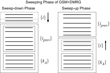
Figure 3: Schematic illustration of the coupling between different configurations during the sweeping phase of GSM+DMRG. Left: sweep-down phase. Here, configurations $\{k_{A}\}$ are coupled with previously generated configurations $\{i_{prev}\}$ and with $\{i\}$ states. Right: sweep-up phase. Here, configurations $\{k_{A}\}$ are coupled with $\{i\}$ and with configurations $\{i_{prev}\}$ in $B$ generated in a previous sweep-down phase.

The representation of $\hat{H}$ in this basis is constructed using the Wigner-Eckart theorem by coupling suboperators acting in $A$, $\{i_{prev}\}$, and $\{i\}$ (the set of states $|i\rangle$). As before, the target state

$$|\Psi_{J}\rangle=\sum_{k,i_{prev},i}c_{k,i_{prev},i}^{J_{part},j_{B}}\{|\Phi_{J_{part}}(k,i_{prev})\rangle\otimes|i(j_{B})\rangle\}^{J}$$ (15)

is identified by picking up the eigenstate of $\hat{H}$ having the largest overlap with the reference state $|\Psi_{J}\rangle^{(0)}$. The density matrix is then constructed

$$\rho^{B}_{ii^{\prime};j_{B}}=\sum_{k,i_{prev},J_{part}}c^{(J_{part},j_{B})}_{k,i_{prev},i}c^{(J_{part},j_{B})}_{k,i_{prev},i^{\prime}}$$ (16)

and diagonalized for each value of $j_{B}$. At this point, the truncation can be done in two different ways. In the first truncation method (i) at most $N_{\rm opt}$ eigenvectors of the density matrix with the largest nonzero moduli of eigenvalues are kept. This is precisely the truncation technique that has been employed in the warm-up phase. The actual number of states retained may vary since one considers only eigenvectors with nonzero eigenvalues. The second method (ii), based on the identity (11), is a generalization of the dynamical block selection approach Leg03 . Here we focus on controlling the numerical error by selecting in each step of the procedure $\rho$, $N_{\rho}$ vectors with the largest moduli of the eigenvalues so that the condition

$$\left|1-Re\left(\sum_{\alpha=1}^{N_{\rho}}w_{\alpha}\right)\right|<\epsilon$$ (17)

is satisfied. The quantity $\epsilon$ in (17) can be viewed as the truncation error of the reduced density matrix. It is worth noting that while the trace of the reduced density matrix is strictly equal to one (11), this is no longer the case for the restricted sum of eigenvalues in (17). In particular, the real part of the reduced trace may be greater than one and the imaginary part may be nonzero. For that reason, in Eq. (17) one considers the real part of the partial trace. The smaller $\epsilon$, the larger number $N_{\rho}$ of eigenvectors must be kept. In particular, for $\epsilon$=0, all eigenvectors with non-zero eigenvalues are retained. One should emphasize that $N_{\rho}$ may change from one step to another. Section IV discusses the convergence of the GSM+DMRG procedure with respect to $N_{\rm opt}$ and $\epsilon$.

The matrix elements (13) in eigenvectors $|\alpha\rangle_{B}$ saved after the truncation are recalculated and stored. The procedure continues by adding the next shells one by one until the first scattering shell is reached. At each step during the sweep-down phase, all suboperators of $\hat{H}$ are stored. The sweep-down phase of GSM+DMRG is schematically illustrated in the left portion of Fig. 3.

At this point, the procedure is reversed, and a sweep in the upward direction (the ‘sweep-up’ phase) begins. Using the information previously stored, a first shell is added, then a second one, etc. (see Fig. 3, right panel). The medium now consists of states in the reference subspace $A$ and states $\{i_{prev}\}$ in $B$ that were generated during a previous sweep-down phase. The sweeping sequences continue until convergence for target eigenvalue is achieved.

IV Applications of the GSM+DMRG method

This work describes the first GSM+DMRG treatment of open-shell proton-neutron nuclei. As illustrative examples, we take ${}^{7}\rm{Li}$ and ${}^{8}\rm{Li}$ described schematically as interacting nucleons outside the closed core of ⁴He. The neutron one-body potential in Eq. (2) is a Woods-Saxon (WS) potential with radius $R_{0}=2$ fm and diffuseness $d=0.65$ fm. The spin-orbit strength $V_{\rm so}=7.5$ MeV and the depth of the central potential $V_{0}$=47 MeV are fixed to reproduce the experimental energies and widths of $3/2_{1}^{-}$ and $1/2_{1}^{-}$ resonances in ⁵He. For the protons, the same WS average potential is supplemented by the Coulomb potential generated by a uniformly charged sphere of radius $R_{0}$ and charge $Q$=+2e.

The two-body interaction in (2) is represented by a finite-range Surface Gaussian Interaction (SGI) Mic04 :

$$V_{i,j}^{J,T} = V_{0}(J,T)\exp\left[-\left(\frac{{\bf{r_{1}}}-{\bf{r_{2}}}}{\mu}\right)^{2}\right]$$ (18)

$$\times \delta(|{\bf{r_{1}}}|+|{\bf{r_{2}}}|-2R_{0}).$$

The strengths $V_{0}(J,T)$ are the same as in Ref. Mic04 . The $T$=0 couplings depend linearly on the number of valence neutrons $N_{v}$:

$$V_{0}^{1,0}=\alpha_{10}-\beta_{10}(N_{v}-1),$$

$$V_{0}^{3,0}=\alpha_{30}-\beta_{30}(N_{v}-1),$$ (19)

where $\alpha_{10}=-600~{}{\rm MeV}\cdot{\rm fm}^{3}$, $\beta_{10}=-50~{}{\rm MeV}\cdot{\rm fm}^{3}$, $\alpha_{30}=-625~{}{\rm MeV}\cdot{\rm fm}^{3}$, and $\beta_{30}=-100~{}{\rm MeV}\cdot{\rm fm}^{3}$.

The above set of parameters has not been optimized to reproduce the actual structure of ⁷Li and ⁸Li. Our choice of interaction is motivated by the fact that the main purpose of this study is to test the DMRG procedure for proton-neutron systems for which the exact GSM diagonalization is still possible. In this context, “our” ⁷Li and ⁸Li systems should be viewed as three- and four-nucleon cases, respectively.

Following the method described in Ref. Mic04 , s.p. bases for protons and neutrons are generated by their respective spherical Hartree-Fock (HF) potentials corresponding to the GSM Hamiltonian (2). Neutron and proton valence spaces include the $0p_{3/2}$ HF poles as well as the scattering shells $\{p_{3/2}\}_{\rm c}$ in the complex $k$-plane, and the $\{p_{1/2}\}_{\rm c}$, $s_{1/2}$, and $d_{5/2}$ real-energy continua.

The $L_{\nu;p_{3/2}}^{+}$ ($L_{\pi;p_{3/2}}^{+}$) contour, along which the scattering $\nu p_{3/2}$ ($\pi p_{3/2}$) shells are distributed, is defined by a triangle with vertices at: $(Re(k),Im(k))=(0.0,0.0),(0.17,-0.1),(2,0.0)$, and a segment along the $Re(k)$-axis from (2.0,0.0) to (8.0,0.0) (in units of fm^-1). Each segment of these contours is discretized with two points corresponding to the abscissa of the Gauss-Legendre quadrature. Hence, we take 6 non-resonant continuum shells from $\{p_{3/2}\}_{\rm c}$ both for protons and neutrons. The real-energy $p_{1/2}$ continuum shells are distributed along the segment [(0,0), (8,0)] which is discretized with 6 points for protons and neutrons. The real-energy $s_{1/2}$ and $d_{5/2}$ continua are included in the valence space as well. They are distributed along the real $k$-axis along the segment [(0,0), (3,0)]. We take six $\{s_{1/2}\}_{\rm c}$ and $\{d_{5/2}\}_{\rm c}$ discretization points, both for protons and neutrons. The $0s_{1/2}$ poles are not included in the valence space as they are assumed to be occupied in the core of ⁴He. The total number of shells $N_{\rm sh}$ in the GSM configuration space is then equal to 50.

IV.1 The three-nucleon case: $J^{\pi}=3/2^{-}$ ground state of ⁷Li

The s.p. basis of ${}^{7}\rm{Li}$ is generated by the HF potential (calculated separately for protons and neutrons and for each partial wave). It contains bound s.p. $p_{3/2}$ states at energies $-$5.605 MeV (neutrons) and $-$7.098 MeV (protons). These s.p. states generate the pole space in the many-body GSM framework and the reference subspace $A$ in DMRG. As discussed above, the total number of resonant ($p_{3/2}$) and non-resonant ($\{p_{3/2}\}_{\rm c}$, $\{p_{1/2}\}_{\rm c}$, $\{s_{1/2}\}_{\rm c}$, $\{d_{5/2}\}_{\rm c}$) shells for protons and neutrons is 50. The dimension of the Lanczos space spanned by one valence proton and two valence neutrons in these 50 shells, i.e., the dimension of the GSM matrix, is $D$=7,796. The ground state energy $E_{\rm ex}=(-26.6620,0.2486)$ MeV has a non-vanishing, unphysical imaginary part. This spurious width comes from the fact that the discretization along the contours is not precise enough to effectively fulfill the completeness relation (1). This problem will be addressed in Sec. IV.1.3 by increasing the number of points along the contour. In what follows, we shall study the convergence of the GSM+DMRG method by varying either the number of eigenvectors $N_{\rm opt}$ kept during the sweeping phase (see Sec. IV.1.1), or the precision $\epsilon$ of the density matrix (see Sec. IV.1.2).

IV.1.1 DMRG truncation with fixed $N_{\rm opt}$

The number of eigenvectors of $\hat{\rho}_{B}$ with the largest nonzero moduli of eigenvalues kept at each iteration during the warm-up phase is limited to ${N}_{\rm opt}^{(0)}$=26. This number corresponds to the total number of states $\{n;j_{B}\}$ in the subspace $B$ that can be coupled with states in $A$ to yield configurations with $J^{\pi}=3/2^{-}$.

The actual number of eigenvectors kept in the warm-up phase may be less than ${N}_{\rm opt}^{(0)}$ since most of eigenvectors have vanishing eigenvalues. The non-resonant continuum shells involved in $B$ are ordered according to the sequence:

$$\{\dots\pi p_{3/2}^{(i)},~{}\nu p_{3/2}^{(i)},~{}\pi p_{1/2}^{(i)},~{}\nu p_{1/2}^{(i)},$$

$$\pi s_{1/2}^{(i)},~{}\nu s_{1/2}^{(i)},~{}\pi d_{5/2}^{(i)},~{}\nu d_{5/2}^{(i)}\dots\},$$ (20)

where index $i$ denotes the position of scattering shells on their respective contours, beginning with those closest to the $k$=0 origin.

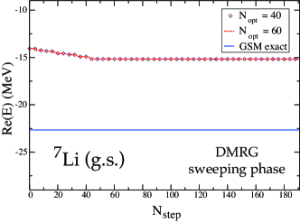
Figure 4: The ground-state energy of ⁷Li as a function of the step number in the sweeping phase, $N_{\rm step}$. For both values of $N_{\rm opt}$, the maximum number of eigenvectors kept during the warm-up phase is $N_{\rm opt}^{(0)}$=26. The step zero corresponds to the result obtained at the end of the warm-up phase. The solid line marks the exact GSM value obtained by means of the direct Lanczos diagonalization.

Figure 4 illustrates the convergence of the GSM+DMRG procedure with respect to the step number in the sweeping phase for $N_{\rm opt}$=40 and 60. The results are identical for both values of $N_{\rm opt}$, and the DMRG ground-state energy converges to the value of $Re(E_{\rm DMRG})=-$15.176 MeV. This exceeds by $\sim$7 MeV the exact GSM value of $Re(E_{\rm ex})$=$-$22.662 MeV, obtained by the direct Lanczos diagonalization of the GSM Hamiltonian.

Clearly, when applied to the case shown in Fig. 4, the GSM+DMRG procedure breaks down. The reason for this failure is not related to a too small value of $N_{\rm opt}$: indeed, in the case $N_{\rm opt}=60$ the largest number of eigenvectors of the density matrix with non-zero eigenvalues is equal to 50. The GSM+DMRG iterative method is trapped in a local minimum, a not uncommon feature of the standard DMRG procedure. A further increase of $N_{\rm opt}$ does not change the final results which is fully converged. To understand the origin of the failure, let us analyze the GSM+DMRG wave function in some detail. To this end, the $J^{\pi}=3/2^{-}$ g.s. wave function of ⁷Li is decomposed as follows:

$$|\Psi\rangle=c_{p^{3}}|p^{3}\rangle+c_{s^{2}p}|s^{2}p\rangle+c_{d^{2}p}|d^{2}p\rangle+c_{spd}|spd\rangle,$$ (21)

where $c_{\nu}$’s are the amplitudes associated with different three-nucleon GSM configurations $|\nu\rangle$. The (real parts) of squared amplitudes $c^{2}_{\nu}$ are shown in Table 1 for the GSM+GDMRG wave function corresponding to $N_{\rm opt}$=60 and for the exact GSM wave function.

Conf.	GSM+DMRG	Exact GSM
$p^{3}$	0.9922	0.9239
$s^{2}p$	0.0003	0.0051
$d^{2}p$	0.0075	0.0644
$spd$	0.0000	0.0066

Table 1: Real part of the squared shell-model amplitudes in the $J^{\pi}=3/2^{-}$ ground state wave function of ⁷Li obtained in GSM+DMRG ($N_{\rm opt}=60$) and through the exact Lanczos diagonalization.

As compared to the exact result, the $|p^{3}\rangle$ parentage amplitude is overestimated and the $|spd\rangle$ component is totally absent in the GSM+DMRG wave function. The latter can be understood by observing that (i) only shells with $l$=1 span the reference subspace $A$, and (ii) during the GSM+DMRG procedure, scattering shells are added one by one. Consequently, when the first positive-parity shell (in our case, a $\pi s_{1/2}$ shell, see (20)) is added, the $|spd\rangle$ component cannot be generated as the first $d_{5/2}$ shell is added only later. When the first $d_{5/2}$ non-resonant shell is included, the $|spd\rangle$ configuration cannot be generated either, because states with one particle in previously considered $s$-shells are not kept in the process of optimization due to the parity conservation. Therefore, the $|spd\rangle$ configuration never enters the DMRG wave function; hence, GSM+DMRG converges to a wrong solution.

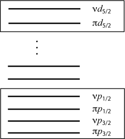
Figure 5: Schematic illustration of the reference subspace $A^{\prime}$ during the warm-up phase of GSM+DMRG for $J^{\pi}=3/2^{-}$ wave functions of ⁷Li. In addition to the $\pi(0p_{3/2})$, $\nu(0p_{3/2})$, $\pi(0p_{1/2})$, and $\nu(0p_{1/2})$ poles, two scattering shells $\pi d_{5/2}$ and $\nu d_{5/2}$ are now included to generate $|spd\rangle$ configurations during the DMRG procedure. See text for more details.

To prevent this pathological behavior, we add to the reference subspace $A$ two positive-parity scattering shells $\pi d_{5/2}$ and $\nu d_{5/2}$ to form a new reference subspace $A^{\prime}$ (see Fig. 5). We arbitrarily choose the last $\pi d_{5/2}$ and $\nu d_{5/2}$ shells in the sequence (20). (As we shall see later, any other positive parity shells can be chosen as well.) The role played by the additional positive parity shells is to generate missing SM couplings in the wave function. The new reference subspace $A^{\prime}$ is used for the construction of the set $\{k_{A^{\prime}}\otimes i_{B}\}$ and the density matrix $\hat{\rho}^{B}$. At each iteration during the warm-up phase, the density matrix contains the correlations due to the additional positive-parity orbits. In this way we assure that no possible couplings are missing during the warm-up phase. We use the same reference state as before, i.e., $|\Psi_{J}^{0}\rangle$ (which is only generated by the resonant shells) to select the target state $|\Psi_{J}\rangle$ among the eigenstates of $\hat{H}$. By the time the first sweep starts, the two shells $(\pi d_{5/2},\nu d_{5/2})$ are included in $B$ and the procedure is carried out as was described in Sec. III with the reference subspace $A$.

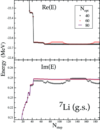
Figure 6: The GSM+DMRG ground state energy (real part, top; imaginary part, bottom) of ⁷Li for $N_{\rm opt}$=40, 60, and 80 as a function of the step number during the sweeping phase. Two non-resonant continuum shells ($\pi d_{5/2},\nu d_{5/2}$) are included in the reference subspace during the warm-up phase ($N_{\rm opt}^{(0)}$=26).

Real and imaginary parts of the ground state energy, obtained using the extended reference subspace $A^{\prime}$ of Fig. 5, are plotted in Fig. 6 for different values of $N_{\rm opt}$. For $N_{\rm opt}$=40, one can see pronounced quasi-periodic oscillations in both real and imaginary parts of the energy. These oscillations have the periodicity of 96 steps corresponding to two consecutive sweeps: sweep-down and sweep-up, each consisting of 48 steps. The energy oscillations rapidly diminish with increasing $N_{\rm opt}$, and the calculated energy $E_{\rm DMRG}$ converges to the GSM benchmark result: $E_{\rm ex}=(-26.6620,0.2486)$ MeV. For $N_{\rm opt}$=80, the deviation from the benchmark result is less than 1 keV for the real part of the energy, and less than 0.1 keV for the corresponding imaginary part.

The rank $d_{\rm H}^{\rm max}$ of largest matrix to be diagonalized grows almost linearly with $N_{\rm opt}$, from $d_{\rm H}^{\rm max}$=716 for $N_{\rm opt}=40$ ($\sim 9.1$ % of the dimension $D$ of the GSM matrix) to $d_{\rm H}^{\rm max}$=1469 ($\sim 19$ % of $D$) for $N_{\rm opt}$=80. One should keep in mind that ${\rm d}_{\rm H}^{\rm max}$ is almost independent of the continuum discretization density Rot2 , i.e., the number of scattering shells considered. Hence, the ratio ${\rm d}_{\rm H}^{\rm max}/D$ decreases rapidly with the number of valence shells Rot2 .

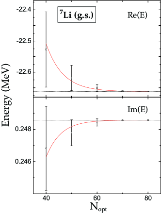
Figure 7: Average value of the ground state energy (top: real part; bottom: imaginary part) of ⁷Li in GSM+DMRG for different values of $N_{\rm opt}$. Error bars correspond to the difference between extremum values of $Re(E_{\rm DMRG})$ (top) and $Im(E_{\rm DMRG})$ (bottom) at the fourth sweep. Two scattering shells ($\pi d_{5/2},\nu d_{5/2}$) are included in the reference subspace during the warm-up phase ($N_{\rm opt}^{(0)}$=26).

The GSM+DMRG energy averaged over steps of the fourth sweep, as well as the minimum and maximum energy value reached during this sweep, are plotted in Fig. 7 for various $N_{\rm opt}$. As $N_{\rm opt}$ increases, the amplitude of energy, defined as the difference between the maximum and the minimum of real (top) or imaginary (bottom) part of GSM+DMRG energy during the fourth sweep, decreases monotonously. Moreover, with increasing $N_{\rm opt}$, both real and imaginary parts of the average energy converge exponentially to the exact value. Results of $\chi^{2}$-analysis are shown by solid lines in Fig. 7. Asymptotic values extracted in this way, $Re(E^{(\infty)}_{\rm DMRG})=-26.6622\pm 0.0002$ MeV and $Im(E_{\rm DMRG}^{(\infty)})=0.248580\pm 0.000004$ MeV, reproduce the exact GSM result very well. The feature of an exponential convergence of the step-averaged GSM+DMRG energies may be useful when estimating eigenvalues based on results obtained with relatively small $N_{\rm opt}$.

To illustrate how the generalized variational principle (6) works, let us consider the energy with the greatest modulus, $E_{\rm max}$, calculated in DMRG during the last sweep. The values of $E_{max}$ and $E_{\rm ave}$, the energy averaged during the last sweep (corresponding to Fig 7), are shown in Table 2 for different $N_{\rm opt}$. One can clearly see that the closer the wave function calculated with DMRG is to the exact wave function as $N_{\rm opt}$ increases, the larger $|E_{\rm max}|$ is. Hence, in this case, the modulus of energy reaches a maximum at the local extremum of the functional $E[\Phi]$ corresponding to the ground state energy of ⁷Li.

The convergence to the exact value is faster by considering $E_{\rm max}$ for each truncation $N_{\rm opt}$ instead of selecting the average value $E_{\rm ave}$ (cf. Table 2). The real part $Re(E_{\rm max})$ converges exponentially to $Re(E^{(\infty)}_{\rm DMRG})=-26.6621\pm 0.0002$ MeV while the imaginary part of $E_{\rm max}$ doesn’t follow the exponential behavior.

$N_{\rm opt}$.	$|E_{\rm max}|$	$Re(E_{\rm max})$	$Im(E_{\rm max})$	$Re(E_{\rm ave})$	$Im(E_{\rm ave})$
40	22.6489	-22.6475	0.2470	-22.5270	0.2468
50	22.6605	-22.6591	0.2484	-22.61844	0.2478
60	22.6631	-22.6617	0.2485	-22.6510	0.2484
70	22.6634	-22.6620	0.2486	22.6609	0.2486
80	22.6634	-22.6620	0.2486	-22.6619	0.2486

Table 2: Modulus, real and imaginary part of $E_{\rm max}$ defined as the DMRG energy with the greatest modulus during the last sweep. The real and imaginary parts of the average energy $E_{\rm ave}$ at the fourth sweep (corresponding to the case presented in Fig 7 are also shown for comparison.

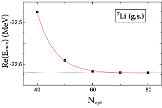
Figure 8: Real part of the ground state energy of ⁷Li as a function of $N_{\rm opt}$. For each $N_{\rm opt}$, the energy with the largest modulus during the last sweep $E_{\rm max}$ is selected. Two scattering shells ($\pi d_{5/2},\nu d_{5/2}$) are included in the reference subspace during the warm-up phase ($N_{\rm opt}^{(0)}$=26).

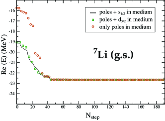
Figure 9: The real part of the ground state energy of ⁷Li as a function of $N_{\rm step}$. The solid line shows results obtained using an extended reference space spanned on the $(p_{3/2},p_{1/2})$ poles space and two ($\pi s_{1/2},\nu s_{1/2}$) scattering shells. Results depicted by squares have been obtained using a standard setup for an extended reference subspace as in Fig. 6. Open circles show results obtained with a reference subspace spanned on the $(p_{3/2},p_{1/2})$ poles and demanding that at least one state from each $\{n;j_{B}\}$ family is kept during the warm-up phase. The values of $N_{\rm opt}^{(0)}$=26 and $N_{\rm opt}$=80 were used in all cases. See text for more details.

The choice of positive-parity scattering shells to be included in the reference subspace is somehow arbitrary. The only important point is that by including both positive and negative parity shells during the warm-up phase, one can generate many-body configurations that would not appear otherwise. For that reason, one can replace $d_{5/2}$ with $s_{1/2}$ scattering shells without changing the outcome of the GSM+DMRG procedure. To illustrate this, Fig. 9 shows the GSM+DMRG results with the extended reference subspace $A^{\prime}$ containing either two $(\pi s_{1/2},\nu s_{1/2})$ or $(\pi d_{5/2},\nu d_{5/2})$ scattering shells. It is seen that the converged value of the GSM+DMRG energy is the same in both cases.

A different way to generate the missing components of the wave function is to demand that at each step during the warm-up phase at least one state from each $\{n;j_{B}\}$ family is kept after truncation. We take up to $N_{\rm opt}^{(1)}$ eigenvectors of the density matrix with largest nonzero eigenvalues, where $N_{\rm opt}^{(1)}$ is equal to the number of different families $\{n;j_{B}\}$ which contribute to the GSM+DMRG wave function. If certain families are not represented in this set of eigenvectors, we add one state for each such family even if the corresponding eigenvalue equals zero. Hence, the actual number of vectors kept during the warm-up phase almost always exceeds $N_{\rm opt}^{(1)}$. Using this additional condition, one may employ a standard setup for the reference subspace (i.e., $A$ is spanned by s.p. poles). Results using this GSM+DMRG strategy are also shown in Fig. 9. The minimal number of states which are kept in the warm-up phase is, in this case, $N_{\rm opt}^{(1)}$=26. In spite of a rather different energy at the beginning of the sweeping phase, the exact GSM+DMRG energy is reproduced. Moreover, the use of an extended reference subspace improves convergence. The rank of the largest matrix to be diagonalized in this case, $d_{\rm H}^{\rm max}$=1469, is independent of the algorithm chosen.

IV.1.2 Truncation governed by the trace of the reduced density matrix

In the examples described in Sec. IV.1.1, the maximum number of states $N_{\rm opt}$ is kept fixed at each step of the sweeping phase. This does not mean that the number of eigenvectors retained in the sweeping phase is always constant or equal $N_{\rm opt}$; only the eigenvectors of the density matrix with non-vanishing eigenvalues are kept. In this section, we shall investigate the GSM+DMRG algorithm in which the number of states $N_{\rho}$ kept at any step in the sweeping phase depends on the condition (17) for the trace of the density matrix. The real part of the $J^{\pi}=3/2^{-}_{1}$ eigenvalue in ⁷Li is shown in Fig. 10 for several values of $\epsilon$. As in the previous examples, the reference subspace $A^{\prime}$ is spanned by the HF poles and two scattering shells $(\pi d_{5/2},\nu d_{5/2})$. In the warm-up phase, we keep $N_{\rm opt}^{(1)}$ eigenvectors of the density matrix (up to 26) and additionally require that at least one state of each $\{n;j_{B}\}$ family is retained. As before, $N_{\rm opt}^{(1)}$ is equal to the number of different $\{n;j_{B}\}$ families so the total number of eigenvectors kept at each iteration step is greater or equal to $N_{\rm opt}^{(1)}$. For low-precision calculations ($\epsilon=10^{-4}$), the resulting energy oscillates and approaches a value which deviates from the correct result by $\sim$1.9 MeV. The amplitude of oscillations as a function of $N_{\rm step}$ quickly decreases with decreasing $\epsilon$. For $\epsilon=10^{-8}$, the precision of the converged GSM+DMRG energy value is $\simeq$ 0.2 keV for both real and imaginary parts.

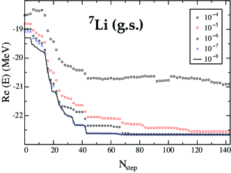
Figure 10: The ground state energy (real part) of ⁷Li as a function of the step number during the sweeping phase for five values of the truncation error $\epsilon$ of the reduced density matrix, see Eq. (17). Two scattering shells ($\pi d_{5/2},\nu d_{5/2}$) are included in the reference subspace during the warm-up phase.

Obviously, the dimension of the largest matrix to be diagonalized depends on the required truncation error $\epsilon$. In the studied case, $d_{\rm H}^{\rm max}$ changes from 273 for $\epsilon=10^{-4}$ to 1327 for $\epsilon=10^{-8}$ with the average number of vectors kept during the sweeping phase increasing from $\sim$15 to $\sim$46. In the truncation scenario with fixed $N_{\rm opt}$, the number of saved vectors, averaged over one sweep, is $\sim$59 for $N_{\rm opt}$=80. In general, for the same precision of GSM+DMRG energies, the average number of vectors kept during the sweeping phase is smaller if the truncation is done dynamically according to the trace of density matrix than by fixing the maximum number of eigenvectors $N_{\rm opt}$.

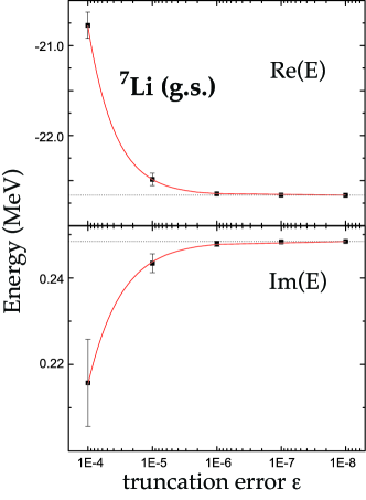
Figure 11: The ground state average energy (top: real part; bottom: imaginary part) of ${}^{7}Li$ as a function of the truncation error $\epsilon$ of the reduced density matrix. Two scattering shells ($\pi d_{5/2},\nu d_{5/2}$) are included in the reference subspace during the warm-up phase. Error bars correspond to a difference between the extremum values of $Re(E_{\rm DMRG})$ at the third sweep. The solid line shows the results of $\chi^{2}$ analysis, assuming power-law convergence (22).

The GSM+DMRG energy averaged over steps of the third sweep as well as the minimum and maximum energy reached during this sweep are plotted in Fig. 11 as a function of $\epsilon$. The GSM+DMRG error, i.e., the energy difference with respect to the exact GSM result, decreases fast with decreasing $\epsilon$. The real and imaginary parts of DMRG energy satisfy to a good approximation the power law

$$Re\left(E_{\rm DMRG}\right)=Re\left(E_{\rm ex}\right)+\alpha\epsilon^{\beta}$$ (22)

proposed in Ref. Leg03 to control the accuracy of the DMRG method for Hermitian problems. The results of a $\chi^{2}$-fit to Eq. (22) are shown in Fig. 11. The asymptotic values extracted in this way are $Re(E^{(\infty)}_{\rm DMRG})=-26.66192\pm 2\cdot 10^{-5}$ MeV and $Im(E_{\rm DMRG}^{(\infty)})=0.24844\pm 3\cdot 10^{-5}$ MeV and agree very well with the exact GSM energy.

In Table 3 we compare the average complex energy $E_{\rm ave}$ at the third sweep for different values of $\epsilon$ (corresponding to Fig 11 and the complex energy $E_{\rm max}$ (the energy with the greatest modulus during the last sweep). As in the previous case where $N_{opt}$ was fixed, the modulus of $E_{\rm max}$ reaches a maximum when $E_{\rm max}$ is equal to the exact GSM energy. As can be seen in Fig. 12, the real part of $E_{\rm max}$ exhibits a power-law behavior with an extrapolated value equal to $Re(E^{(\infty)}_{\rm DMRG})=-26.660.5\pm 0.0012$ MeV.

$\epsilon$.	$|E_{\rm max}|$	$Re(E_{\rm max})$	$Im(E_{\rm max})$	$Re(E_{\rm ave})$	$Im(E_{\rm ave})$
$10^{-4}$	20.9221	-20.9209	0.2240	-20.7751	0.2157
$10^{-5}$	22.5575	-22.5562	0.2416	-22.4870	0.2434
$10^{-6}$	22.6532	-22.6519	0.2485	-22.6474	0.2479
$10^{-7}$	22.6621	-22.6607	0.2481	-22.6602	0.2483
$10^{-8}$	22.6632	-22.6618	0.2486	-22.6618	0.2484

Table 3: Modulus, real and imaginary part of $E_{\rm max}$ defined as the energy having the greatest modulus during the last sweep. The real and imaginary parts of the average energy $E_{average}$ at the fourth sweep (see Fig 11) are also shown for comparison.

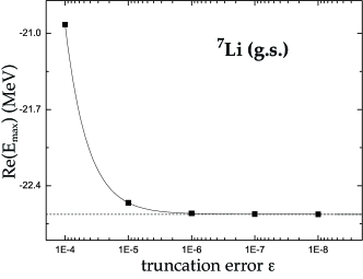
Figure 12: Real part of the ground state energy of ⁷Li as a function of $\epsilon$. At each $\epsilon$, the energy is selected according to the greatest modulus during the last sweep.

IV.1.3 Treatment of spurious width

As mentioned in Sec. IV.1, the imaginary part of the GSM energy $E_{\rm ex}=(-26.6620,0.2486)$ MeV is non-physical for it has a negative width. This is due to the fact that the contour discretization is not sufficiently precise to guarantee the completeness relation (1). This spuriosity can be taken care of by increasing the number of points along the integration contour. In the largest calculation we have done for the ground state of ⁷Li, we took 67 points along the contour $L_{\pi;p_{3/2}}^{+}$, 24 along $L_{\pi;p_{3/2}}^{+}$, and 12 points along the contours $L_{\pi;s_{1/2}}^{+}$ and $L_{\pi;d_{5/2}}^{+}$. The neutron valence space is the same as the proton space except for the contour $L_{\nu;p_{3/2}}^{+}$ where 74 points are considered. The model space corresponds to 239 shells and the dimension of the ground state $J^{\pi}=3/2^{-}$ GSM Hamiltonian matrix is 1,459,728.

In order to perform calculations within this huge valence space, we have developed a parallel version of the DMRG code. At each step during the DMRG procedure, calculations of the matrix elements of the suboperators (7) and hamiltonian (2) are distributed among the processors. Our calculations were carried out on the CRAY XT4 Jaguar supercomputer at the Oak Ridge National Laboratory.

The real part of the ground state energy and the fit according to the relation (22) are plotted in Fig 13. For each $\epsilon$ the energy $E_{\rm max}$ with the greatest modulus during the third sweep is considered. The extrapolated value is $Re(E^{(\infty)}_{\rm DMRG})=-21.6834\pm 0.0010$ MeV. The real part of $E_{max}$ for $\epsilon=5\cdot 10^{-10}$ is -21.6820  MeV and the amplitude during the last sweep is 2.275  keV; hence, convergence has almost been reached. Here, the largest matrix has a dimension 3,348. The imaginary part (which does not follow the power law behavior) varies from 0.00100  MeV at $\epsilon=10^{-7}$ to 0.00075  MeV at $\epsilon=5\cdot 10^{-10}$ (its amplitude during the last sweep is 0.065  keV). This example nicely demonstrates the validity of the many-body completeness relation in GSM.

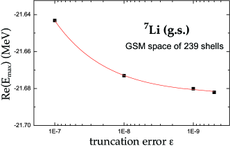
Figure 13: Real part of the ground state energy of ⁷Li in a model space made of 239 shells. At each $\epsilon$, the energy is selected according to the greatest modulus during the third sweep. See text for details.

IV.2 The four-nucleon case: $J^{\pi}=2^{+}$ ground state of ⁸Li

The GSM Hamiltonian for ⁸Li is the same as for ⁷Li, the only modification being the change of $T$=0 couplings in Eq. (19) due to the different number of neutrons $N_{v}$=3. The HF procedure yields two bound s.p. states: $e_{p_{3/2}}=-8.556$ MeV and $e_{p_{3/2}}=-12.788$ MeV, for neutrons and protons, respectively. Shells of the non-resonant continuum are distributed in the complex $k$-plane using the same contours and the same discretization scheme as in the ⁷Li case. The dimension of the Lanczos space spanned by one valence proton and three valence neutrons in 50 shells, i.e., the dimension of the GSM matrix in ⁸Li, is $D$=170,198. The GSM+DMRG results presented in this section are obtained using the truncation criterion (17). As discussed in Sec. IV.1.2, this criterion is somewhat more efficient than the condition based on fixing the maximum number of eigenvectors $N_{\rm opt}$.

The truncation method employed in the warm-up phase follows that of Sec. IV.1.1. The reference subspace $A^{\prime}$ is spanned by the pole states and two scattering shells ($\pi d_{5/2},\nu d_{5/2}$). We take up to 50 eigenvectors of the density matrix with the largest nonzero eigenvalues. If certain $\{n;j_{B}\}$ families are not represented in this set of eigenvectors, we add one state for each such family even if the corresponding eigenvalue equals zero. In the sweeping phase, we follow the truncation strategy of Sec. IV.1.2.

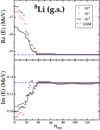
Figure 14: The real part of the ground state energy of ⁸Li as a function of step number during the sweeping phase. Results are shown for different values of the truncation error $\epsilon$. Two non-resonant continuum shells ($\pi d_{5/2},\nu d_{5/2}$) are included in the reference subspace during the warm-up phase.

Figure 14 shows the DMRG+GSM results for ⁸Li for three values of $\epsilon$. The exact energy of the $2^{+}_{1}$ state obtained by the direct Lanczos diagonalization of the GSM matrix is $E_{\rm ex}=(-19.19451,0.13361)$ MeV. The corresponding energies averaged over the third sweep are plotted in Fig. 15. For $\epsilon=10^{-4}$, the largest matrix to be diagonalized has a rank $d_{\rm H}^{\rm max}$=1,446 ($\sim 0.8$% of $D$). For $\epsilon=10^{-8}$, one obtains $E_{\rm DMRG}=(-19.19415,0.13355)$ MeV, i.e. the real part of the GSM+DMRG energy deviates only by 0.4 keV from the exact value, while for the imaginary part, the deviation is less than 0.06 keV. The largest matrix to be diagonalized in this case has a rank ${\rm d}_{\rm H}^{\rm max}$=20,535 ($\sim 12$ % of $D$).

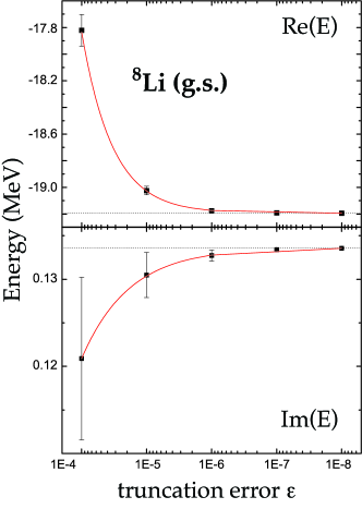
Figure 15: Similar as in Fig. 11 except for the ground state average energy of ⁸Li.

V Conclusions

This work describes the first application of the DMRG method to two-fluid, open many-fermion systems represented by complex-symmetric Hamiltonians. Calculations were carried out for proton-neutron systems ⁷Li (three-nucleon problem) and ⁸Li (four-nucleon problem). As compared to our previous work Rot2 , two significant improvements of the GSM+DMRG technique have been made. The first improvement concerns the recognition of the appropriate target state in the warm-up phase. The second development relates to the truncation strategy in the sweeping phase.

There are situations in which the DMRG procedure yields a fully converged but incorrect solution. In order to understand and prevent this pathological behavior, we studied a necessary and sufficient condition for the GSM+DMRG method to yield a correct eigenvalue. The essential condition is to assure that all possible couplings in the many-body wave function, allowed by the symmetries of the problem and the configuration space, are present in the warm-up phase. We propose different strategies to guarantee this crucial requirement.

Two truncation schemes for the number of retained vectors in the sweeping phase of DMRG were investigated: the fixed-$N_{\rm opt}$ scheme (Sec. IV.1.1) and the dynamic truncation (Sec. IV.1.2). We conclude that the two strategies are to a large extent equivalent; they both exhibit the excellent convergence properties to the benchmark GSM result. In both cases, one finds the quasi-periodic oscillations of GSM+DMRG energy as a function of $N_{\rm step}$ with extensive plateaux.

The GSM+DMRG energy averaged over one sweep exhibits excellent exponential convergence with $N_{\rm opt}$ which allows to deduce the asymptotic value with good precision. Also, $E_{\rm DMRG}$ exhibits excellent convergence as a function of the truncation error $\epsilon$. This feature makes it possible to control the accuracy of GSM+DMRG calculations.

The dynamic truncation, fixing a condition on the trace of the reduced density matrix, yields results of similar accuracy for ⁷Li and ⁸Li, i.e., for systems having very different configuration spaces. This offers a possibility to compare the convergence in different quantal systems at the same value of $\epsilon$.

The encouraging features of the proposed GSM+DMRG approach open the window for systematic and high-precision studies of complex, weakly bound nuclei, such as halo systems, which require large configuration spaces involving s.p. states of different parities (both in the pole space and in the scattering space). Generally, the improvements of the DMRG approach proposed in this work can be of interest in the context of other multiparticle open quantum systems, as well as for other DMRG calculations involving non-Hermitian Hamiltonians.

VI Acknowledgements

We thank Gaute Hagen for usefull discussions. This work was supported by the U.S. Department of Energy under Contract Nos. DE-FG02-96ER40963 (University of Tennessee), DE-AC05-00OR22725 with UT-Battelle, LLC (Oak Ridge National Laboratory), and DE-FG05-87ER40361 (Joint Institute for Heavy Ion Research), by the Spanish DGI under grant No. FIS2006-12783-c03-01, and by the CICYT-IN2P3 cooperation. Computational resources were provided by the National Center for Computational Sciences at Oak Ridge and the National Energy Research Scientific Computing Facility.

References

- (1) J. Dobaczewski and W. Nazarewicz, Phil. Trans. R. Soc. Lond. A 356, 2007 (1998).
- (2) J. Okołowicz, M. Płoszajczak, and I. Rotter, Phys. Rep. 374, 271 (2003).
- (3) J. Dobaczewski, N. Michel, W. Nazarewicz, M. Płoszajczak, and J. Rotureau, Prog. Part. Nucl. Phys. 59, 432 (2007).
-
(4)
K. Bennaceur, F. Nowacki, J. Okołowicz and M. Płoszajczak, Nucl. Phys. A 651,289 (1999);
K. Bennaceur, F. Nowacki, J. Okołowicz, and M. Płoszajczak, Nucl. Phys. A 671, 203 (2000). -
(5)
J. Rotureau, J. Okołowicz, and M. Płoszajczak, Phys. Rev. Lett. 95, 042503 (2005);
J. Rotureau, J. Okołowicz, and M. Płoszajczak, Nucl. Phys. A 767, 13 (2006). - (6) A. Volya and V. Zelevinsky, Phys. Rev. C 74, 064314 (2006).
-
(7)
N. Michel, W. Nazarewicz, M. Płoszajczak, and K. Bennaceur, Phys. Rev. Lett. 89, 042502 (2002);
N. Michel, W. Nazarewicz, M. Płoszajczak, and J. Okołowicz, Phys. Rev. C 67, 054311 (2003). -
(8)
R. Id Betan, R.J. Liotta, N. Sandulescu, and T. Vertse, Phys. Rev. Lett. 89, 042501 (2002);
R. Id Betan, R.J. Liotta, N. Sandulescu, and T. Vertse, Phys. Rev. C 67, 014322 (2003). - (9) R. Id Betan, R.J. Liotta, N. Sandulescu, and T. Vertse, Phys. Lett. B 584, 48 (2004).
- (10) N. Michel, W. Nazarewicz, M. Płoszajczak, and J. Rotureau, Phys. Rev. C 74, 054305 (2006).
- (11) G. Hagen, M. Hjorth-Jensen, and N. Michel, Phys. Rev. C 73, 064307 (2006).
-
(12)
T. Berggren, Nucl. Phys. A 109, 265 (1968);
T. Berggren and P. Lind, Phys. Rev. C 47, 768 (1993). - (13) S.R. White, Phys. Rev. Lett. 69, 2363 (1992); Phys. Rev. B 48, 10345 (1993).
- (14) J. Dukelsky and S. Pittel, Rep. Prog. Phys. 67, 513 (2004).
- (15) U. Schollwöck, Rev. Mod. Phys. 77, 259 (2005).
- (16) K. Hallberg, Adv. Phys. 55, 477 (2006).
- (17) S.R. White and R. L. Martin, J. Chem Phys. 110, 4127 (1999).
- (18) D. Ghosh, J. Hachmann, T. Yanai, and G.K. Chan, J. Chem. Phys. 128 144117 (2008).
- (19) J. Dukelsky and G. Sierra, Phys. Rev. Lett. 83, 172 (1999).
- (20) D. Gobert, U. Schollwöck, and J. von Delft, Eur. Phys. J. B 38, 501 (2004).
- (21) N. Shibata and D. Yoshioka, Phys. Rev. Lett. 86, 5755 (2001).
- (22) Y. Weiss and R. Berkovits, Solid State Commun. 145, 585 (2008).
- (23) J. Dukelsky, S. Pittel, S.S. Dimitrova, and M.V. Stoitsov, Phys. Rev. C 65, 054319 (2002).
- (24) A.E. Feiguin, E. Rezayi, C. Nayak, and S. Das Sarma, Phys. Rev. Lett. 100, 166803 (2008).
- (25) E. Carlon, M. Henkel, and U. Schollwöck, Eur. J. Phys. B 12, 99 (1999).
- (26) T. Papenbrock and D.J. Dean, J. Phys. G 31, S1377 (2005).
- (27) S. Pittel and N. Sandulescu, Phys. Rev. C 73, 014301 (R) (2006).
- (28) S. Pittel, B. Thakur, and N. Sandulescu, arXiv:0808.1303 (2008).
- (29) J. Rotureau, , N. Michel, W. Nazarewicz, M. Płoszajczak, and J. Dukelsky, Phys. Rev. Lett. 97, 110603 (2006).
- (30) N. Moiseyev, P.R. Certain, and F. Weinhold, Mol. Phys. 36, 1613 (1978).
- (31) N. Moiseyev, Phys. Rep. 302, 212 (1998).
- (32) N. Moiseyev, Chem. Phys. Lett. 99, 364 (1983).
- (33) Ö. Legeza, J. Röder, and B.A. Hess, Phys. Rev. B 67, 125114 (2003).
- (34) Y. Suzuki and Wang Jing Ju, Phys. Rev. C 41, 736 (1990).
- (35) N. Michel, W. Nazarewicz, and M. Płoszajczak, Phys. Rev. C 70, 064313 (2004).
- (36) I. McCulloch and M. Gulacsi, Europhys. Lett. 57, 852 (2002).