Magnetically-Regulated Fragmentation Induced by Nonlinear Flows and Ambipolar Diffusion
Abstract
We present a parameter study of simulations of fragmentation regulated by gravity, magnetic fields, ambipolar diffusion, and nonlinear flows. The thin-sheet approximation is employed with periodic lateral boundary conditions, and the nonlinear flow field (“turbulence”) is allowed to freely decay. In agreement with previous results in the literature, our results show that the onset of runaway collapse (formation of the first star) in subcritical clouds is significantly accelerated by nonlinear flows in which a large-scale wave mode dominates the power spectrum. In addition, we find that a power spectrum with equal energy on all scales also accelerates collapse, but by a lesser amount. For a highly super-Alfvénic initial velocity field with most power on the largest scales, the collapse occurs promptly during the initial compression wave. However, for trans-Alfvénic perturbations, a subcritical magnetic field causes a rebound from the initial compression, and the system undergoes several oscillations before runaway collapse occurs. Models that undergo prompt collapse have highly supersonic infall motions at the core boundaries. Cores in magnetically subcritical models with trans-Alfvénic initial perturbations also pick up significant systematic speeds by inheriting motions associated with magnetically-driven oscillations. Core mass distributions are much broader than in models with small-amplitude initial perturbations, although the disturbed structure of cores that form due to nonlinear flows does not guarantee subsequent monolithic collapse. Our simulations also demonstrate that significant power can (if present initially) be maintained with negligible dissipation in large-scale compressive modes of a magnetic thin sheet, in the limit of perfect flux freezing.
keywords:
ISM: clouds , ISM: magnetic fields , MHD , stars: formationPACS:
97.10.Bt , 98.38.Am , 98.38.Dq, , , and
1 Introduction
Magnetic fields and supersonic turbulence are two mechanisms that are commonly invoked for the regulation of star formation in our Galaxy to the observationally estimated rate of yr-1 (see McKee, 1989). This is at least one hundred times less than the rate implied by the gravitational fragmentation timescale of the molecular gas in the Galaxy calculated from its mean density. Put another way, the global Galactic star formation efficiency (SFE) is about 1% of molecular gas per free-fall time. Interestingly, the same SFE also applies to nearby individual star-forming regions such as the Taurus molecular cloud (Goldsmith et al., 2008). The relatively low Galactic SFE is one fundamental constraint on the global properties of star formation. The existence of a broad-tailed core mass function (CMF) that is a lognormal with a possible power-law high-mass tail, is another. In fact, the observed form of the CMF (e.g. Motte et al., 1998) is similar to that of the stellar initial mass function, the IMF. Other important star formation constraints specifically applying to cores include the generally subsonic relative infall motions (Tafalla et al., 1998; Williams et al., 1999; Lee et al., 2001; Caselli et al., 2002), the low (subsonic or transonic) systematic core speeds (André et al., 2007; Kirk et al., 2007), and the somewhat non-circular projected shapes (Myers et al., 1991; Jones et al., 2001). The relatively low speeds are an important property since the cores are embedded in molecular clouds whose overall internal random motions are highly supersonic.
Since most stars form in clusters or loose groups, it seems clear that some sort of fragmentation process is at work in those regions. There are several qualitatively distinct modes of fragmentation to consider. The simplest process is gravitational fragmentation, which can be divided into cases with mass-to-flux ratios that are supercritical (gravity-dominated) and subcritical (ambipolar-diffusion-driven). An alternate and distinct star formation mechanism is turbulent fragmentation, dominated by nonlinear flows, which can also occur in clouds with supercritical and subcritical mass-to-flux ratios. The limit of highly supercritical clouds also corresponds to super-Alfvénic turbulence in the case that turbulent and gravitational energies have comparable magnitude. This limit has been advocated by Padoan & Nordlund (2002). However, we favor the transcritical and trans-Alfvénic cases on theoretical and observational grounds, as discussed in Section 4. For a more complete understanding of star formation, a study of the interplay of magnetic fields, turbulence, and ambipolar diffusion is therefore of great importance. In this paper, we carry out an extensive parameter survey of magnetic field strengths and initial nonlinear perturbations, facilitated by our use of the thin-sheet approximation, and discuss the consequences of our results. Such broad parameter studies remain out of reach for fully three-dimensional non-ideal MHD simulations (Kudoh & Basu, 2008; Nakamura & Li, 2008).
In a previous paper (Basu et al. 2009, hereafter BCW; see also Basu & Ciolek 2004), we studied the nonlinear evolution of gravitational fragmentation initiated by small-amplitude perturbations, including the effects of magnetic fields and ambipolar diffusion. An extensive parameter study was performed, encompassing the supercritical, transcritical, and subcritical cases, and also accounting for varying levels of cloud ionization and external pressure. Some main findings of that paper were that fragment spacings in the nonlinear phase agree with the predictions of linear theory (Ciolek & Basu, 2006), and that the time to runaway collapse from small-amplitude white-noise initial perturbations is up to ten times the growth time calculated from linear theory. Ciolek & Basu (2006) showed that transcritical gravitational fragmentation can lead to significantly larger size and mass scales than either the supercritical or subcritical limits. BCW found that CMFs for regions with a single uniform initial mass-to-flux ratio are sharply peaked, but that the sum of results from simulations with a variety of initial mass-to-flux ratios near the critical value can produce a broad distribution. This represents a way to get a broad CMF, of the type observed, without the need for nonlinear forcing. Importantly, only a narrow initial distribution of initial mass-to-flux ratio is needed to create a relatively broad CMF. Additionally, BCW showed that different ambient mass-to-flux ratios in different regions lead to observationally distinguishable values of infall motions, core shapes, and magnetic field line curvature. Kudoh et al. (2007) have recently performed three-dimensional simulations of gravitational fragmentation with magnetic fields and ambipolar diffusion, and verified some of the main findings of the thin-sheet models. Particularly, they also found the dichotomy between subsonic maximum infall speeds in subcritical clouds and somewhat supersonic speeds in supercritical clouds.
The inclusion of nonlinear (hereafter, “turbulent”) initial conditions to fragmentation models including ambipolar diffusion was introduced by Li & Nakamura (2004) and Nakamura & Li (2005), employing the thin-sheet approximation. They found that the timescale of star formation was reduced significantly by the initial motions with power spectrum (Li & Nakamura, 2004), to become yr for an initially somewhat subcritical cloud rather than yr. By continuing to integrate past the collapse of the first core through the use of an artificially stiff equation of state for surface densities 10 times greater than the initial value, they found that magnetic fields nevertheless prevented most material from collapsing to form stars. Kudoh & Basu (2008) have verified that the mode of turbulence-accelerated magnetically-regulated star formation also occurs in a fully three-dimensional simulation. While three-dimensional simulations are resource-limited, and large parameter studies cannot yet be performed, Kudoh & Basu (2008) showed that this mode of star formation proceeds though an initial phase of enhanced ambipolar diffusion created by the small length scale generated by the large-scale compression associated with the initial perturbation. If this is not sufficient to raise the maximum mass-to-flux ratio above the critical value, there is a rebound to lower densities. However, the highest density regions remain well above the initial mean density, and here the ambipolar diffusion proceeds in a quasistatic manner ( assuming force balance between gravity and magnetic forces - see Mouschovias & Ciolek 1999) but at an enhanced rate due to the raised density.
In this paper, we study the effect of large-amplitude nonlinear initial perturbations on the evolution of a thin sheet whose evolution is regulated by magnetic fields and ambipolar diffusion. We focus on the early stages of prestellar core formation and evolution, and do not integrate past the runaway collapse of the first core. Therefore, the effects of protostellar feedback through outflows do not need to be added. These simplifications allow us to run a large number of simulations. We perform an extensive parameter study and also study many realizations of models with a single set of parameters, since the initial turbulent state is inherently random. Some important questions that we can address and which have not been answered in previous papers are as follows. In which parameter space do nonlinear velocity fields lead to prompt collapse, and in which cases can magnetic fields cause a rebound from the first compressions? How sensitively does the time until runaway collapse depend upon the values of different parameters? What is the effect of different power spectra of perturbations? Is there a qualitative difference between Alfvénic and super-Alfvénic perturbations? How do velocity profiles in the vicinity of cores vary in the different scenarios? What are the systematic speeds of cores?
Our paper is organized in the following manner. The model is described in Section 2, results are given in Section 3, and a discussion of results, including speculation and implications for global star formation in a molecular cloud are given in Section 4. We summarize our results in Section 5.
2 Physical and Numerical Model
We employ the magnetic thin-sheet approximation, as laid out in detail in several previous papers (Ciolek & Mouschovias, 1993; Ciolek & Basu, 2006; Basu et al., 2009). Physically, we are modeling the dense mid-layer of a molecular cloud, and ignoring the more rarefied envelope of the cloud. We assume isothermality at all times. The basic equations governing the evolution of a model cloud (conservation of mass and momentum, Maxwell’s equations, etc.) are integrated along the vertical axis from to . In doing so, a “one-zone approximation” is used, in which all quantities are taken to be independent of height within the sheet. The volume density of neutrals is calculated from the vertical pressure balance equation
| (1) |
where is the isothermal sound speed, is the column density of neutrals, is the external pressure on the sheet, and and represent values of magnetic field components at the top surface of the sheet, .
We solve normalized versions of the magnetic thin-sheet equations. The unit of velocity is taken to be , the column density unit is , and the unit of acceleration is , equal to the magnitude of vertical acceleration above the sheet. Therefore, the time unit is , and the length unit is . From this system we can also construct a unit of magnetic field strength, . The unit of mass is . Here, is the uniform neutral column density of the background state. Typical values of our units are given in the Appendix. With these normalizations, the equations used to determine the evolution of a model cloud are
| (2) | |||||
| (3) | |||||
| (4) | |||||
| (5) | |||||
| (6) | |||||
| (7) | |||||
| (8) | |||||
| (9) | |||||
| (10) | |||||
| (11) | |||||
| (12) | |||||
| (13) | |||||
| (14) |
In the above equations, is the planar magnetic field at the top surface of the sheet, is the velocity of the neutrals in the plane, and is the corresponding velocity of the ions. The operator is the gradient in the planar directions within the sheet. The quantities and are the scalar gravitational and magnetic potentials in the plane of the sheet, derived in the limit that the sheet is infinitesimally thin. The vertical wavenumber is a function of wavenumbers and in the plane of the sheet, and the operators and represent the forward and inverse Fourier transforms, respectively, which we calculate numerically using an FFT technique. Terms of order in , the magnetic force per unit area, are not written down for the sake of brevity, but are included in the numerical code; their exact form is given in Sections 2.2 and 2.3 of Ciolek & Basu (2006). All terms proportional to are generally very small.
The Eq. (7) above makes use of relations for the neutral-ion collision time and the ion density , as described in BCW:
| (15) | |||||
| (16) |
Furthermore, Eq. (7) uses the normalized initial mass density (in units of ) , where is defined below.
Our basic equations contain three dimensionless free parameters: is the dimensionless (in units of the critical value for gravitational collapse) mass-to-flux ratio of the reference state; is the dimensionless neutral-ion collision time of the reference state, and expresses the effect of ambipolar diffusion; is the ratio of the external pressure acting on the sheet to the vertical self-gravitational stress of the reference state.
Each numerical model is carried out within a square computational domain spanning the region and . Periodic boundary conditions are imposed in the and directions. We choose a domain size for all models presented in this paper, so that it is four times wider than the wavelength of maximum growth rate for an isothermal nonmagnetic and unpressured sheet, (see Ciolek & Basu 2006; BCW). The computational domain has zones in each direction, with unless stated otherwise. Some results utilizing greater are presented in Section 3.4.
Gradients in our simulation box are approximated using second-order accurate central differencing. Advection of mass and magnetic flux is prescribed by using the monotonic upwind scheme of van Leer (1977). These forms of spatial discretization convert the system of partial differential equations to a system of ordinary differential equations (ODE’s), with one ODE for each physical variable at each cell. Time-integration of this large coupled system of ODE’s is performed by using an Adams-Bashforth-Moulton predictor-corrector subroutine (Shampine, 1994). Numerical solution of Fourier transforms and inverse transforms, necessary to calculate the gravitational and magnetic potentials and at each time step (see Eqs. [12] and [14]), is done by using fast Fourier transform techniques. Further details of our numerical technique are given by BCW.
The initial conditions of our model include a “turbulent” velocity field added to our background state of uniform column density and vertical magnetic field strength . The velocity field is generated in Fourier space using the usual practice adopted by e.g. Stone et al. (1998) for three-dimensional models and Li & Nakamura (2004) for thin-sheet models. For a physical grid consisting of zones in each direction, the wavenumbers and in Fourier space consist of the discrete values , where . For each pair of and , we assign a Fourier velocity amplitude chosen from a Gaussian distribution and scaled by the power spectrum , where . The phase is chosen from a uniform random distribution in the interval . The resulting Fourier velocity field is then transformed back into physical space. The distributions of each of and are chosen independently in this manner, and each is rescaled so that the rms amplitude of the field is equal to . For , the resulting velocity field has most of its power in a large-scale flow component. We have experimented with various values of and find that the results are generally similar as long as . Distinct results are found in the case of flat spectrum perturbations (), which we present for comparison. Finally, we note that velocity fields generated in the above manner are compressive. Hence, we have also studied one model with but the Fourier space amplitudes chosen so that and satisfy .
Therefore, our turbulent initial conditions introduce the additional dimensionless free parameters and , while our simulation box introduces the parameters and grid size .
3 Results
| Model | Spectrum | ||||||
|---|---|---|---|---|---|---|---|
| 1 | 0.5 | 0.0 | 0.1 | 2.0 | 2.9 | ||
| 2 | 0.5 | 0.2 | 0.1 | 4.0 | 2.9 | 0.8 | |
| 3 | 0.5 | 0.2 | 0.1 | 3.0 | 2.9 | 30 | |
| 4 | 0.5 | 0.2 | 0.1 | 2.0 | 2.9 | 31 | |
| 5 | 0.5 | 0.2 | 0.1 | 1.0 | 2.9 | 50 | |
| 6 | 0.5 | 0.2 | 0.1 | 0.5 | 2.9 | 58 | |
| 7 | 0.5 | 0.2 | 10.0 | 2.0 | 1.0 | 8.5 | |
| 8 | 0.5 | 0.2 | 0.1 | (div0) | 2.0 | 2.9 | 23 |
| 9 | 0.5 | 0.2 | 0.1 | 2.0 | 2.9 | 56 | |
| 10 | 0.5 | 0.1 | 0.1 | 2.0 | 2.9 | 92 | |
| 11 | 0.5 | 0.4 | 0.1 | 2.0 | 2.9 | 8.1 | |
| 12 | 0.5 | 1.0 | 0.1 | 2.0 | 2.9 | 1.8 | |
| 13 | 1.0 | 0.2 | 0.1 | 2.0 | 1.7 | 1.8 | |
| 14 | 1.0 | 0.2 | 0.1 | 1.0 | 1.7 | 4.3 | |
| 15 | 1.0 | 0.2 | 0.1 | 0.5 | 1.7 | 12 | |
| 16 | 1.0 | 0.2 | 0.1 | 2.0 | 1.7 | 33 | |
| 17 | 2.0 | 0.2 | 0.1 | 2.0 | 1.2 | 1.3 |
Table 1 contains a summary of models in our parameter study. For each model, we list the values of the free parameters , the form of the turbulent power spectrum, the turbulent velocity amplitude , the magnetosound speed in the initial state of the model, and the calculated duration of the simulation, . The initial magnetosound speed is calculated from the other parameters of the model, and its relation to can act as a useful diagnostic. Following Ciolek & Basu (2006) we use
| (17) |
where is the square of the normalized (to ) initial Alfvén speed, and is the square of a normalized initial effective sound speed that includes the effect of external pressure, and follows from Eq. (8). Model 7 has because for , the large external pressure contributes significant opposition to the restoring force of internal pressure in the initial state (see discussion in Ciolek & Basu, 2006).
Our simulations are terminated as soon as , corresponding to runaway gravitational collapse of the first core. For models with , this also corresponds to a volume density enhancement by a factor . We have verified with high resolution runs to greater values of that the collapse does indeed continue. Collapsing regions are also invariably gravity-dominated, having locally supercritical mass-to-flux ratios and net accelerations that point toward the density peak. This includes cases of prompt collapse, i.e. when collapse occurs in localized regions due to strong shocks associated with the turbulent flow field, in a time less than . The values of do vary somewhat from one realization of the initial state to another, and in many cases represent an average value from many simulations. We have run each model at least five separate times, and some have been run significantly many more times, as described below. Model 1, which evolves under flux-frozen conditions (), cannot be terminated in the usual manner. Since the initial mass-to-flux ratio is also subcritical for this model (), gravitational runaway collapse is not possible unless there is significant numerical magnetic diffusion. That simulation ran past without runaway collapse or any notable artificial flux dissipation, thus providing an excellent verification of the accuracy of our code. While some models undergo many oscillations before eventual runaway collapse of density peaks, others undergo prompt collapse. Although the models that undergo prompt collapse may be considered to be artificially forced into collapse by large-scale flows in the initial conditions, we nevertheless present them here as interesting limiting cases. Models 4, 13, and 17 constitute a special set of models with our standard neutral-ion coupling parameter , external pressure , turbulent velocity amplitude , but varying initial mass-to-flux ratio parameter , respectively. Model 4 is run 15 times, and models 13 and 17 are run 25 times (with unique random realizations of the initial velocity field), in order to compile statistics on the core mass distributions using the techniques described by BCW. Model 4 can in some sense be considered our “standard” model since we are most interested in the acceleration of collapse in subcritical clouds due to nonlinear supersonic velocity perturbations. Model 8 is similar to model 4 but has the divergence-free initial velocity field. Model 3 is on the brink of either prompt collapse or a longer-term evolution leading to runaway collapse, and can sometimes go into prompt collapse (see Section 4). For this reason, we ran the model over 15 times in order to yield a that is a characteristic value for all but a few runs that do go into prompt collapse.
3.1 Global Properties
 |
 |
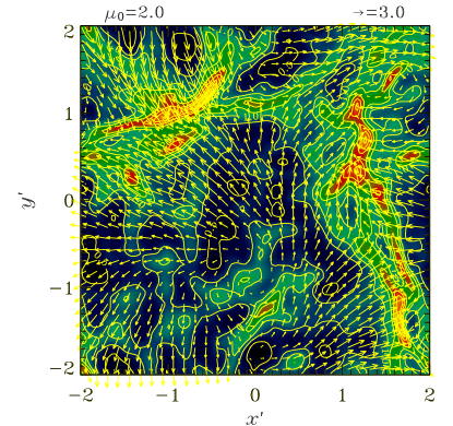 |
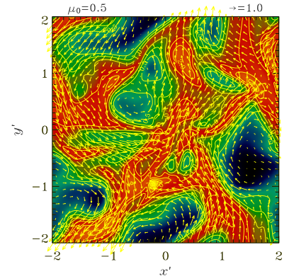
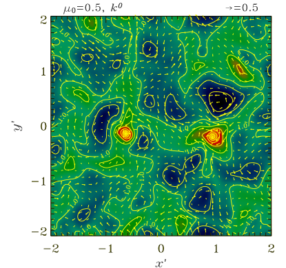
Fig. 1 shows images of column density overlaid with column density contours and velocity vectors, for realizations of models 4 (top left), 13 (top right), and 17 (bottom left). Each snapshot is at the end of the simulation, when , but occurs at a different time , as indicated in Table 1. The maximum speeds in the simulation region are quite different at the end of the three simulations even though all three start with perturbations characterized by . Therefore, the velocity vector plots each have a different normalization, with the horizontal or vertical distance between footpoints of vectors corresponding to , , and for the three models with , and respectively. To understand the difference in maximum speeds, it is important to understand the different course of evolution in each model.
The model 4, with , has a strong enough magnetic field that the initial compression driven by the large-scale flow of the nonlinear velocity field does not lead to prompt collapse in any region. The magnetic field causes a rebound after the initial compression. The densest regions never reexpand fully to the initial background density, and instead undergo oscillations in density until continuing ambipolar diffusion leads to the creation of regions of supercritical mass-to-flux ratio. These regions then undergo runaway collapse. For model 4, this occurs at a representative , meaning that there is sufficient time for the initial velocity field to have damped significantly, since we do not replenish turbulent energy in these simulations. This is why the velocity amplitude is much smaller at the end of the simulation than in the other two runs. However, the maximum value is still supersonic (), and there are strong systematic flow fields in the simulation. In contrast, when starting with small-amplitude initial perturbations (BCW), the maximum infall speeds are subsonic. In that case, runaway collapse also occurred much later, at . The color table and column density contours for model 4, when compared to those for models 13 and 17, reveal that the gas is not as compressed and filamentary as in those cases, due to the rebound from the initial extreme compressions.
The images, contours, and velocity vectors for models 13 () and 17 () reveal that the initial strong compression leads to immediate runaway collapse within highly compressed filaments. The velocity field has highly ordered supersonic compressive infall motions. The runaway collapse is occurring at times and , respectively, essentially as soon as the initial flow creates a large-scale compression. Although kinetic energy is efficiently dissipated behind the shock fronts, there is hardly enough time for a large reduction of the global kinetic energy. Therefore, the maximum speeds at the end of the simulation ( for model 13 and for model 17) are quite similar to the initial maximum values.
 |
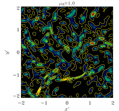 |
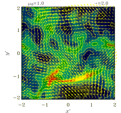
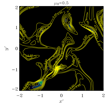
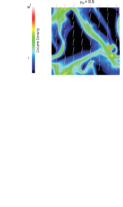
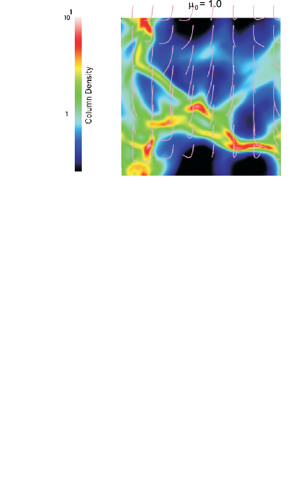
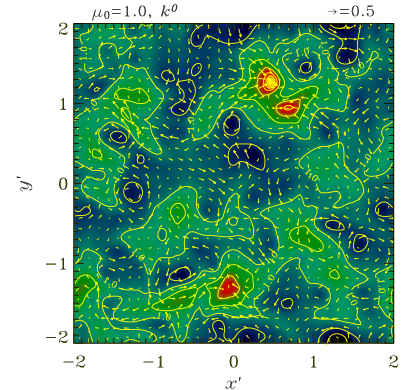
Fig. 2 shows images of the mass-to-flux ratio at the end of the simulations of models 4 and 13. The end states have a combination of subcritical and supercritical regions. Subcritical regions are shown in black, and a color table is applied to the supercritical regions on both panels. The left panel illustrates that the supercritical regions of the initially significantly subcritical () cloud are created within the filamentary regions generated by the large-scale compressions. In contrast, the initially critical () model has widespread supercritical regions generated by the small-scale modes of turbulence, as well as the most supercritical regions in the compressed layers. The former effect of widespread patches of mildly supercritical gas is possible due to the marginal nature of the critical () initial state. Physically, we might expect the cloud with to lead to a cluster of stars soon after the runaway collapse of the first cores. On the other hand, the significantly subcritical cloud with would show only isolated star formation in the compressed layers and have to wait a much longer time before ambipolar diffusion leads to clustered star formation in the remainder of the cloud.
 |
 |
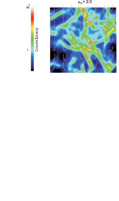 |
Fig. 3 shows the end states of models 4, 13, and 17 in different realizations (i.e. starting with a different but statistically equivalent initial velocity field) than shown in Fig. 1. A color table shows the column density of the final state, and magnetic field lines above the sheet are also illustrated. These lines are generated in the manner described in BCW. The image of sheet surface and field lines above are viewed from an angle of from the sheet normal direction. Animations of the evolution of the sheet surface density, with field lines appearing in the last frame, are available online. Clearly, the models which suffer prompt collapse ( and ) show the most curvature of field lines since the field is dragged inward by the strong initial compression wave. In contrast, the cloud with (top left) undergoes a rebound and several oscillations before runaway collapse can occur. This allows the magnetic field to straighten out again. The ultimate collapse of the first core is due to ambipolar drift of neutrals past field lines, so the field is not significantly distorted by this process. However, a legacy of the initial compression is that the mass-to-flux ratio is no longer spatially uniform, and significant column density structure exists even if the magnetic field is not very distorted.
The relative amounts of field line curvature in the cloud and within dense cores are quantified by , where is the magnitude of the planar magnetic field at any location on the sheet-like cloud. Hence, is the angle that a field line makes with the vertical direction at any location at the top or bottom surface of the sheet. To quantify the differences in field line bending from subcritical to transcritical to supercritical clouds, we note that representative realizations of models 4, 13, and 17, with , have average values , and maximum values (probing the most evolved core in each simulation) . Of these, only the model with shows similar values of as a corresponding model with initial small-amplitude perturbations. For models with small-amplitude initial perturbations, BCW found that yields representative values , and .
 |
 |
 |
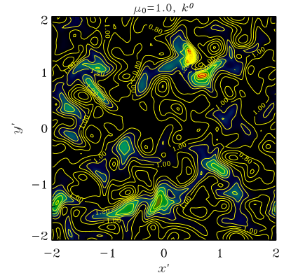 |
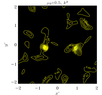
The evolution of models with flat spectrum () initial perturbations is distinct from the cases with negative exponent, so we present the results from models 9 and 16 in Fig. 4. In these models, as in model 4, but the large-scale flow does not dominate the initial condition. Therefore, the small-scale modes contribute more significantly to enhance ambipolar diffusion. This enhancement of ambipolar diffusion due to small-scale irregularities is similar to the mechanism studied analytically by Fatuzzo & Adams (2002) and Zweibel (2002). We study only models with and in order to focus on the enhanced ambipolar diffusion. The values of for these models are and respectively. These are significantly longer time scales than in the corresponding models with . However, they are much shorter than in models with the same background state and linear initial perturbations (studied by BCW), in which case is and for and , respectively.
Fig. 4 shows the column density and mass-to-flux ratio at the end of simulations of model 9 and 16. The input turbulence acts to increase the rate of ambipolar diffusion, but the turbulence also decays away. By the time of runaway collapse, the cloud structure and kinematics more closely resembles the case of small-amplitude initial perturbations than the case of nonlinear-flow-induced fragmentation (models 4 and 13). Representative values of the maximum speed of neutrals at the time of runaway collapse are for model 9 and for model 16. Both values are closer to the values and when starting with small-amplitude initial perturbations (BCW) than for the cases of nonlinear-flow-induced fragmentation, in which case and , respectively. The bottom panels show the mass-to-flux ratio at the end of simulations of model 9 and 16. The subcritical model 9 has only isolated pockets of supercritical cores, as well as emerging cores which still have subcritical but enhanced mass-to-flux ratio. The image is similar to the corresponding image when starting with small-amplitude perturbations (Fig. 9 of BCW), but the cores are not circular in shape. The fragmentation scale also seems related to that of the small-amplitude perturbation model, although many fragments are just beginning to emerge and may take a much longer time to develop fully. The corresponding image for model 16 shows that the initially critical () state leads to many regions of supercritical mass-to-flux ratio. The emerging fragment pattern has less resemblance to the corresponding case that starts from small amplitude perturbations (Fig. 9 of BCW) than for . Nevertheless, a fragmentation scale is more apparent than for the case of nonlinear-flow-induced fragmentation shown in Fig. 2. The relatively low amount of remaining turbulence at the end of both simulations means that new cores will develop on the non-accelerated ambipolar diffusion time scale, leading to a significant age spread of star formation. In the nonlinear initial condition models, with or spectrum, we may identify the initial cores with an early phase of star formation that is induced by turbulence, and the emerging cores with a later phase of star formation that can grow from lingering small-amplitude perturbations. In this way, our model could be in qualitative agreement with the empirical scenario advocated by Palla & Stahler (2000).
3.2 Time Evolution


Fig. 5 shows the time evolution of maximum column density for four models and of the maximum mass-to-flux ratio for three models, all having . It clearly shows that for subcritical clouds: (1) fragmentation by runaway collapse does not occur under conditions of flux-freezing (dash-dotted line; the simulation actually runs past without runaway collapse); (2) small-amplitude (linear) perturbations result in the classical quasistatic evolution requiring a time ; (3) flat spectrum () nonlinear perturbations that result in a collapse time that is shorter by a factor ; (4) power-law () spectrum nonlinear perturbations that result in a rapid collapse that is shorter than the linear case by a factor . Of course, the exact values of will depend on and other parameters such as and . For the fourth case above, it may depend on the box size as well, since that sets the scale of the largest mode in the simulation. This figure corresponds to Fig. 1 of Kudoh & Basu (2008), which shows results for some three-dimensional models. In their figure, the volume density and plasma (counterparts to and in our thin-sheet model) undergo some variations due to vertical oscillations of the cloud, before eventually increasing rapidly. Our model follows the integrated quantities through the layer and therefore does not include the effect of vertical oscillations. Nevertheless, the timescale of evolution and eventual runaway collapse are in good agreement where comparisons can be made. Our thin-sheet model allows a broader parameter study than currently possible using three-dimensional simulations.
Fig. 6 shows the time evolution of maximum column density and maximum mass-to-flux ratio for three models with . The model with small amplitude (linear) initial perturbations corresponds to model 3 of BCW. The other ones are model 13 and model 16 of this paper. The same three qualitatively distinct evolutionary modes occur as for the case of . A notable difference is that collapse occurs immediately during the first compression in the case of nonlinear-flow-induced fragmentation, at . There is no rebound from the first compression as occurs when .
Fig. 7 illustrates the effect of varying levels of ionization on the fate of nonlinear-flow-induced fragmentation. This is represented by differing values of , with corresponding to flux-freezing and differing values of corresponding to different initial ionization fractions (see Appendix). The standard model with corresponds to a canonical ionization fraction (Tielens, 2005). Our results show that may indeed vary significantly due to variations in , easily spanning the range of yr to yr for typical values of units and input parameters. Clearly, a definitive understanding of the influence of magnetic fields awaits further insight into ionization levels in molecular clouds.
3.3 Core Properties
Two important observed properties of dense cores are the kinematics of infall motions, and the distribution of core masses. The latter suffers from some ambiguity due to the different possible definitions of a “core”, or more specifically, how to define a core “boundary”. Here we describe the most basic features of our simulated cores.
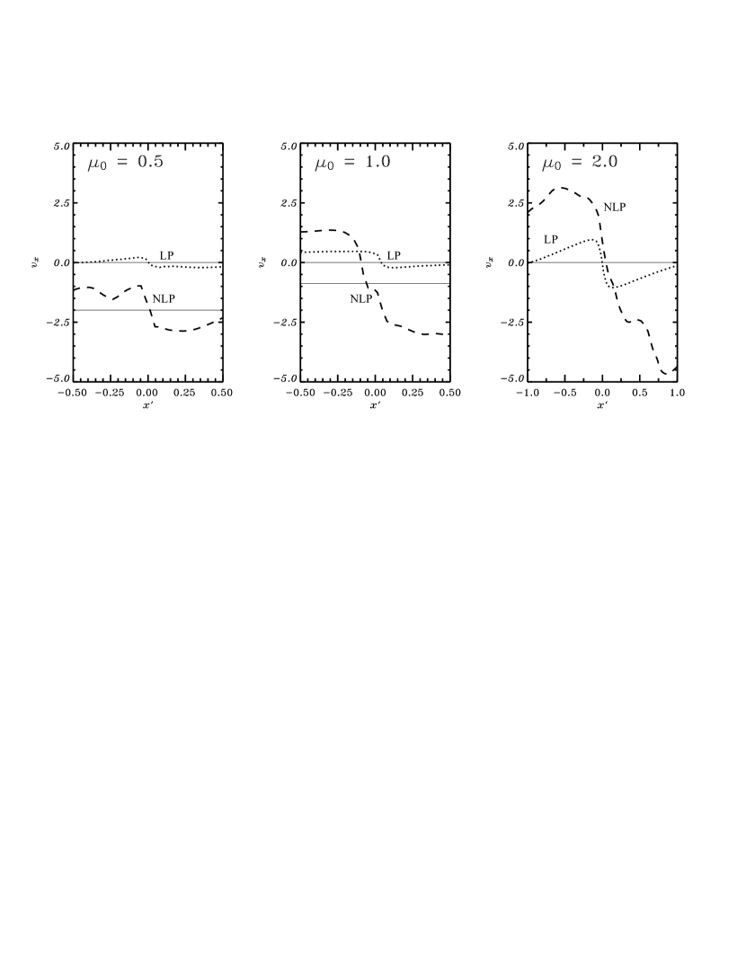
Fig. 8 shows the velocity profiles (using dashed lines) in the vicinity of cores that are obtained in simulations of models 4, 13, and 17, with , and 2.0, respectively. They are measured along a line in the -direction that passes through the column density peak. Also shown (in dotted lines) for each value of is a profile of -velocity through a core that is formed in a simulation with small-amplitude (linear) perturbations (BCW), but otherwise the same parameters as the other model shown in the same panel. The horizontal solid lines in each panel pass through the “midplane” of the velocity profiles, and allow one to read off the systematic -velocity of the core. For the cases of initial linear perturbations, the increasing sequence of leads to ever increasing maximum infall speeds, from about half the sound speed up to mildly supersonic values. There is also evidence of infall speeds increasing towards the core centers, due to gravitational acceleration. For the cases of initial nonlinear perturbations (these models all have a spectrum), the sequence of increasing leads to greater relative infall speeds onto the cores. These motions are supersonic in all cases, and constitute an important observationally-testable consequence of nonlinear-flow-induced fragmentation. The models with greater have greater infall speeds because they undergo collapse during the first compression, with most of the initial input turbulent energy still intact, i.e. there has not been much time for turbulent decay. Also note that there is no evidence for an accelerating flow in these cases, which would be a signature of gravitationally-driven motions. Thus, these models demonstrate flow-driven core formation, rather than gravitationally-driven core formation. For the model with there is essentially no systematic core speed, since the collapse occurs very quickly at the intersection of two colliding flows. At the other limit of a significantly subcritical cloud (), the initial compression is followed by a rebound due to the strong magnetic restoring forces. The core forms later within the region of high density that is undergoing oscillatory motions. The systematic speed of the core relative to the simulation box is supersonic (about twice the sound speed in this model), although the relative speed of infall onto the core is subsonic or transonic. The large systematic core speeds for subcritical clouds constitute another observationally-testable consequence of nonlinear-flow-induced fragmentation. The case of is intermediate in features between the and models, but is actually closer to the model since the collapse occurs very quickly, with . This is very close to the value for the model.
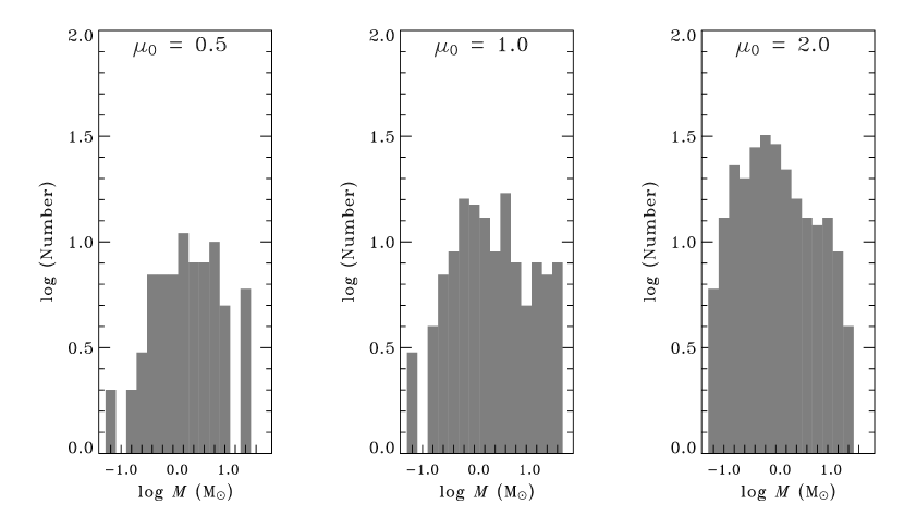
Fig. 9 shows the histograms of core masses, defined as masses enclosed within regions that have surrounding a column density peak. These are measured at the end of each simulation, for 15 separate realizations of model 4, and 25 each of models 13 and 17. Simulations of model 4 () and model 13 () produce an average of five identifiable cores per simulation, while model 17 () produces an average of ten cores per simulation. For details about our thresholding technique used to obtain core masses, see BCW. The histograms reveal that for any fixed value of , the distribution of core masses is much broader than the corresponding histogram of masses for fixed and initial small-amplitude (linear) perturbations. See Fig. 8 of BCW for the latter, which show a very sharp descent beyond the preferred mass scale. There are many more high-mass cores that are formed in these models. However, an examination of Figs. 1 and 3 reveals that many of the cores have very elongated and irregular shapes, so that they may yet break up into multiple fragments. In BCW, we proposed that a broad CMF may be caused by a distribution of initial mass-to-flux ratio values within a cloud. That remains an alternative scenario to that of “turbulent fragmentation” explored here and in several previous publications (Padoan et al., 1997; Klessen, 2001; Gammie et al., 2003; Tilley & Pudritz, 2007).
3.4 Turbulent Dissipation

The rate of dissipation of turbulent energy has been studied extensively in a series of three-dimensional simulations (e.g. Stone et al., 1998; Mac Low et al., 1998; Mac Low, 1999; Ostriker et al., 2001). See also the reviews by Mac Low & Klessen (2004), Elmegreen & Scalo (2004), and McKee & Ostriker (2007). In this Section, our goal is to briefly present some information about the turbulent decay in our simulations. These may be of interest because our simulations differ in their use of the thin-sheet approximation and the use of high-order adaptive time-stepping that is part of our implementation of the method of lines technique (see BCW). Nevertheless, we do also obtain relatively rapid turbulent dissipation in most models, as presented in the various figures in this Section.
We present results for the decay of kinetic energy in our simulation box. However, the total energy in the simulation box is not conserved, due to radiative losses implied by our isothermal assumption, and also due to work done by the external pressure and magnetic forces associated with the field components and at the cloud’s top and bottom surfaces. Nevertheless, the amount of turbulent kinetic energy present in a cloud has important observational implications, so we illustrate its evolution here in several figures. We also use the kinetic energy evolution as a means of exploring the effect of numerical resolution in our simulations.
Fig. 10 shows the evolution of kinetic energy (defined as the sum of over all cells of a simulation), normalized to initial values , for models 4, 6, and 13. Note that the values of differ from model to model. The model with does not have much chance to lose kinetic energy because collapse occurs right away, during the first turbulent compression. For models with , there is a rebound from the initial compression, and this is indicated by the oscillations of . Furthermore, there is an overall systematic decay of so that it is significantly reduced in one sound crossing time of the initial half-thickness of the cloud, , where we have used Eq. (30) of BCW to relate to . The decaying oscillations of are consistent with the qualitative picture obtained from the animation of model 4 that accompanies Fig. 3. Some of our realizations do show an increase in during the last stage of evolution, due to the conversion of gravitational energy into kinetic energy of systematic infall onto one or more cores.
Fig. 11 shows the effect of resolution on the decay of kinetic energy. Our standard simulations have , and numerical experiments with and demonstrate that while some more kinetic energy is retained in those cases, the overall pattern of decay and oscillations of is maintained. We note that each simulation has a unique random but statistically equivalent initial state.
Fig. 12 reveals the additional effect on the kinetic energy evolution of two interesting limits. In one case, we perform the numerical experiment of starting with a divergence-free (non-compressive) initial velocity field, even though turbulence in the interstellar medium is thought to be highly compressive (McKee & Ostriker, 2007). For this case, a plot of for the evolution of model 8 (dashed line) reveals that the kinetic energy still decays, but that the cloud does not undergo large-scale oscillations during the process. These oscillations occur in the compressible case due to the restoring force of the magnetic field when compressed into filamentary structures. This does not occur in the incompressible model in a globally coherent manner, although locally compressive motions are generated during the evolution and turbulent decay does occur rapidly, as in the other models. The dash-dotted line reveals the interesting evolution in the case of flux-freezing (model 1; ). Here the initially compressive velocity field leads to an initial rapid decay of turbulence through shocks, but large-scale oscillatory modes remain in the simulation box for indefinite periods of time. These modes have a root mean squared velocity amplitude and contain roughly half the initial input energy. Why do these modes not decay away? The lack of ambipolar diffusion means there is no dissipation of modes in which the restoring force is due to the magnetic field. The spectrum means that the largest modes dominate, and these also suffer negligible numerical dissipation in our scheme. The restoring force that drives the waves is provided largely by the magnetic tension associated with the magnetic field external to the sheet. While the case of a thin sheet may not be generalizable to three dimensional molecular clouds, we feel this result is an important pointer to processes that may in fact be occurring in real clouds. That is, the external magnetic field, anchored in the Galactic interstellar medium, may allow the outer parts of clouds (effectively flux-frozen due to UV ionization - see Ciolek & Mouschovias 1995) to maintain long-lived oscillations that are then identified observationally as “turbulence”. This idea has long been advocated by Mouschovias (1975, 1987). We note that this result could not be obtained in periodic box simulations that contain no effect of an external medium, and leave a more thorough assessment of this effect to a forthcoming paper.


4 Discussion
We have performed a parameter study of fragmentation of a dense sheet aided by the presence of initial nonlinear velocity perturbations. In most models, the power spectrum of fluctuations is , so that the initial conditions impose primarily a large-scale flow to the system. We have also studied the case of nonlinear perturbations with power spectrum , in which the small-scale fluctuations play a bigger role. Of the two modes, the latter is more similar to gravitational fragmentation arising from small-amplitude perturbations, as studied extensively in our previous paper (BCW). The main difference is an accelerated time scale for core formation. This is particularly apparent for the cases with subcritical initial mass-to-flux ratio, in which case the nonlinear fluctuations enhance ambipolar diffusion (see Fatuzzo & Adams, 2002; Zweibel, 2002). For the case of nonlinear-flow-induced fragmentation, originally studied by Li & Nakamura (2004) and Nakamura & Li (2005), we find that the induced structures are highly filamentary and go into direct collapse for supercritical clouds. For critical, and more so for subcritical clouds, the initial compression may be followed by a rebound and oscillations which eventually lead to runaway collapse in dense pockets where enhanced ambipolar diffusion has created supercritical conditions. What determines the outcome? For any given field strength, there is a threshold initial velocity amplitude above which prompt collapse will take place. An examination of model outcomes in Table 1 reveals that, for a fixed standard initial ionization fraction defined by , prompt collapse takes place when (see models 2, 13, and 17). Indeed, the model 3, which has , is actually prone to go into prompt collapse () in some realizations, but undergoes several oscillations before runaway collapse in most cases (with representative value ). We can say that significantly super-Alfvénic perturbations are associated with prompt collapse, for both subcritical and supercritical model clouds. This criterion does not apply to models with initial power spectrum , since the kinetic energy does not get channeled toward a large-scale compression wave. It also does not apply to model 7 (), since its low value of is very specific to the external-pressure-dominated initial state, but not representative of the signal speed in the high-density regions that are subsequently generated.
The highly filamentary structure of clouds in which prompt collapse takes place is a source of concern when comparing with maps of observed molecular clouds. This was noted by Li & Nakamura (2004), who commented that clouds with weak magnetic field and supersonic turbulence as modeled (i.e. power spectrum, having most power on the largest scales) would appear too filamentary in comparison with observations. Our study extends this concern also to models with strong magnetic field if the turbulence is highly super-Alfvénic, since prompt collapse occurs in highly compressed filaments without a chance for them to rebound. Since the weak magnetic field cases also have by design a velocity amplitude that is super-Alfvénic, we can say that super-Alfvénic turbulence in all cases may have problems with excessive filamentarity. There is another problem with large amounts of turbulent forcing; the relative infall motions onto the cores are highly supersonic (see Fig. 8), and at odds with observed core infall motions (Tafalla et al., 1998; Williams et al., 1999; Lee et al., 2001; Caselli et al., 2002), which are subsonic or at best transonic. Of course, both of these problems are set up artificially in our simulations through nonlinear forcing associated with the initial conditions. In other simulations of driven super-Alfvénic turbulence (Padoan & Nordlund, 2002), such forcing continues at all times and the above features are always present.
If the highly turbulent and/or super-Alfvénic models pose difficulties for dense core formation, then how does one account for the highly supersonic motions observed in molecular clouds (e.g. Solomon et al., 1987)? The answer is likely that they exist in the lowest density envelopes of the molecular clouds and therefore should not be input into local models of dense subregions, as we do in some cases here. Our super-Alfvénic models in a periodic simulation box demonstrate a limiting case, and help establish that such models cannot be applied directly to explain observed star-forming regions. In a global scenario, the dense regions that form cores will be less turbulent than the larger low-density envelopes. The low-density regions can support highly turbulent motions while denser regions have lower velocity dispersion, as demonstrated in 1.5 dimensional global models of molecular cloud turbulence (Kudoh & Basu, 2003, 2006).
Our Fig. 9 shows that the core mass distribution is relatively broad for any given value of for nonlinear-flow-induced fragmentation ( spectrum of velocity fluctuations). This repeats the qualitative findings of many earlier studies in three-dimensions (Padoan et al., 1997; Klessen, 2001; Gammie et al., 2003; Tilley & Pudritz, 2007). This scenario of turbulent fragmentation is a plausible mechanism to generate broad CMFs of the type observed. It remains an open question whether this kind of CMF is related to the IMF since the cores are often highly irregular in shape, and it is not clear that they will collapse monolithically. Alternative methods to generate broad IMFs or CMFs are the global effect of competitive accretion (Bonnell et al., 2003; Bate et al., 2003), a temporal spread of core accretion lifetimes (Myers, 2000; Basu & Jones, 2004), or a distribution of initial mass-to-flux ratios in a cloud (BCW). Future work by the astrophysical community may clarify the relative roles of these processes.
5 Summary
We have studied the effect of initial nonlinear velocity perturbations on the formation of dense cores in isothermal sheet-like layers that may be embedded within larger molecular cloud envelopes. Our simulation box is periodic in the lateral () directions and typically spans four nonmagnetic (Jeans) fragmentation scales in each of these directions. The initial input turbulent energy is allowed to decay freely. The simulations reveal a wide range of outcomes. We emphasize the following main results of the paper:
-
1.
Time Evolution to Runaway. Subcritical model clouds can undergo accelerated ambipolar diffusion in two different ways. For nonlinear initial velocity perturbations in which small-scale modes contain a large portion of the energy, the onset of runaway collapse occurs sooner by a factor in our typical models. For nonlinear perturbations with most energy on the largest scales (hereafter, nonlinear flows), the runaway collapse can be sped up by a greater factor, for our typical models. Supercritical clouds undergo prompt collapse whenever nonlinear flows are present. Subcritical model clouds may also be pushed into prompt collapse by nonlinear flows that are significantly super-Alfvénic.
-
2.
Morphology of Clouds. Supercritical model clouds whose evolution is initiated by nonlinear flows have a highly filamentary structure. Subcritical clouds with initial nonlinear but trans-Alfvénic or sub-Alfvénic flows have a markedly less filamentary structure. In these cases, magnetic fields cause a rebound from the initial compression, and several oscillations occur before the runaway collapse of the first cores. Subcritical clouds with initially super-Alfvénic nonlinear flows promptly develop highly filamentary structure with embedded collapsing cores.
-
3.
Velocity Profiles. Supercritical and transcritical model clouds which are driven into prompt collapse have highly supersonic infall speeds at the core boundaries, while subcritical model clouds typically have transonic or subsonic infall speeds (relative to the velocity centroid) onto cores. In the subcritical cases, the cores can have larger systematic motions than in supercritical models, because the cores form within regions undergoing oscillatory motions. We believe that the large infall motions in the models with super-Alfvénic nonlinear flows may disqualify them as viable models for core formation, given current observational results.
-
4.
Core Mass Distributions. Core formation initiated by nonlinear flows leads to broader core mass functions than found in earlier studies of fragmentation initiated by small-amplitude perturbations. This applies to models of any fixed initial mass-to-flux ratio . However, the ultimate relation of such a core mass function to the stellar initial mass function is not settled due to the irregular shape of the fragments created by nonlinear flows. These fragments may in turn break up into multiple objects at a later stage.
-
5.
Turbulent Decay. Supersonic initial velocity perturbations lead to an initially rapid decay of kinetic energy in all models, on a time scale similar to the sound crossing time across the half-thickness of the sheet. This rapid decay of turbulence is in agreement with a wide variety of previous results in the literature. However, subcritical model clouds can undergo oscillations that reduce the decay rate of kinetic energy at later times. Furthermore, in the limit of excellent neutral-ion coupling (flux-freezing), as may be present in UV-ionized molecular cloud envelopes, large-scale wave modes may survive for very long times.
Acknowledgements
We thank the anonymous referee for comments which improved the discussion of results. We also thank Stephanie Keating for creating color images and animations using the IFRIT package developed by Nick Gnedin. SB was supported by a grant from the Natural Sciences and Engineering Research Council (NSERC) of Canada. JW was supported by an NSERC Undergraduate Summer Research Award.
Appendix A Typical Values of Units and Other Quantities
Typical values of our units are
| (18) | |||||
| (19) | |||||
| (21) | |||||
| (22) |
Here, we have used , where is the mean molecular mass of a neutral particle for an H2 gas with a 10% He abundance by number. Furthermore, we may calculate the number density of the background state as
| (23) |
The dimensional background reference magnetic field strength for a given model is simply . Finally, the ionization fraction () in the cloud may be expressed as
| (24) |
References
- André et al. (2007) André, P., Belloche, A., Motte, F., Peretto, N. 2007. A&A 472, 519.
- Basu & Ciolek (2004) Basu, S., Ciolek, G. E. 2004. ApJ 607, L39.
- Basu et al. (2009) Basu, S., Ciolek, G. E., Wurster, J. 2009. NewA 14, 221 (BCW).
- Basu & Mouschovias (1995) Basu, S., Mouschovias, T. Ch. 1995. ApJ 453, 271.
- Basu & Jones (2004) Basu, S., Jones, C. E. 2004. MNRAS 347, L47.
- Bate et al. (2003) Bate, M. R., Bonnell, I. A., Bromm, V. 2003. MNRAS 339, 577.
- Bonnell et al. (2003) Bonnell, I. A., Bate, M. R., Vine, S. G. 2003. MNRAS 343, 413.
- Caselli et al. (2002) Caselli, P., Walmsley, C. M., Zucconi, A., Tafalla, M., Dore, L., Myers, P. C. 2002. ApJ 565, 331.
- Ciolek & Basu (2006) Ciolek, G. E., Basu, S. 2006. ApJ 652, 442.
- Ciolek & Mouschovias (1993) Ciolek, G. E., Mouschovias, T. Ch. 1993. ApJ 454, 194.
- Ciolek & Mouschovias (1995) Ciolek, G. E., Mouschovias, T. Ch. 1995. ApJ 418, 774.
- Elmegreen & Scalo (2004) Elmegreen, B. G., Scalo, J. 2004. ARAA 42, 211.
- Fatuzzo & Adams (2002) Fatuzzo, M., Adams, F. C. 2002. ApJ 570, 210.
- Gammie et al. (2003) Gammie, C. F., Lin, Y.-T., Stone, J. M., Ostriker, E. C. 2003. ApJ 592, 203.
- Goldsmith et al. (2008) Goldsmith, P. F., Heyer, M., Narayanan, G., Snell, R., Li, D., Brunt, C. 2008. ApJ 680, 428.
- Jones et al. (2001) Jones, C. E., Basu, S., Dubinski, J. 2001. ApJ 551, 387.
- Kirk et al. (2007) Kirk, H., Johnstone, D., Tafalla, M. 2007. ApJ 668, 1042.
- Klessen (2001) Klessen, R. S. 2001. ApJ 556, 837.
- Kudoh & Basu (2003) Kudoh, T., Basu, S. 2003. ApJ 595, 842.
- Kudoh & Basu (2006) Kudoh, T., Basu, S. 2006. ApJ 642, 270.
- Kudoh & Basu (2008) Kudoh, T., Basu, S. 2008. ApJ 679, L79.
- Kudoh et al. (2007) Kudoh, T., Basu, S., Ogata, Y., Yabe, T. 2007. MNRAS 380, 499.
- Lee et al. (2001) Lee, C. W., Myers, P. C., Tafalla, M. 2001. ApJS 136, 603.
- Li & Nakamura (2004) Li, Z.-Y., Nakamura, F. 2004. ApJ 609, L83.
- McKee (1989) McKee, C. F. 1989. ApJ 345, 782.
- McKee & Ostriker (2007) McKee, C. F., Ostriker, E. C. 2007. ARAA 45, 565.
- Mac Low et al. (1998) Mac Low, M.-M., Klessen, R. S., Burkert, A., Smith, M. D. 1998. Phys. Rev. Lett. 80, 2754.
- Mac Low (1999) Mac Low, M.-M. 1999. ApJ 524, 169.
- Mac Low & Klessen (2004) Mac Low, M.-M., Klessen, R. S. 2004. Rev. Mod. Phys. 76, 125.
- Motte et al. (1998) Motte, F., André, P., Neri, R. 1998. A&A 336, 150.
- Mouschovias (1975) Mouschovias, T. Ch. 1975. PhD Thesis. Berkeley.
- Mouschovias (1987) Mouschovias, T. Ch. 1987. In: Morfil, G., Scholer, M. (Eds.), Physical Processes in Interstellar Clouds. Reidel, Dordrecht, p. 453.
- Mouschovias & Ciolek (1999) Mouschovias, T. Ch., Ciolek, G. E. 1999. In: Lada, C. J., Kylafis, N. (Eds.), The Origin of Stars and Planetary Systems. Kluwer, Dordrecht, p. 305.
- Myers (2000) Myers, P. C. 2000. ApJ 530, L119.
- Myers et al. (1991) Myers, P. C., Fuller, G. A., Goodman, A. A., Benson, P. J. 1991. ApJ 376, 561.
- Nakamura & Li (2005) Nakamura, F., Li, Z.-Y. 2005. ApJ 631, 411.
- Nakamura & Li (2008) Nakamura, F., Li, Z.-Y. 2008. ApJ 687, 354.
- Ostriker et al. (2001) Ostriker, E. C., Stone, J. M., Gammie, C. F. 2001. ApJ 546, 980.
- Padoan et al. (1997) Padoan, P., Nordlund, A., Jones, B. J. T. 1997. MNRAS 288, 145.
- Padoan & Nordlund (2002) Padoan, P., Nordlund, A. 2002. ApJ 576, 870.
- Palla & Stahler (2000) Palla, F., Stahler, S. W. 2000. ApJ 540, 255.
- Shampine (1994) Shampine, L. F. 1994. Numerical Solution of Ordinary Differential Equations. Chapman & Hall, New York.
- Solomon et al. (1987) Solomon, P. M., Rivolo, A. R., Barrett, J., Yahil, A. 1987. ApJ 319, 730.
- Stone et al. (1998) Stone, J. M., Gammie, C. F., Ostriker, E. C. 1998. ApJ 508, L99.
- Tafalla et al. (1998) Tafalla, M., Mardones, D., Myers, P. C., Caselli, P., Bachiller, R., Benson, P. J. 1998. ApJ 504, 900.
- Tielens (2005) Tielens, X. 2005. The Physics and Chemistry of the Interstellar Medium. Cambridge Univ. Press, Cambridge.
- Tilley & Pudritz (2007) Tilley, D. A., & Pudritz, R. E. 2007. MNRAS 382, 73.
- van Leer (1977) van Leer, B. 1977. JCP 23, 276.
- Williams et al. (1999) Williams, J. P., Myers, P. C., Wilner, D. J., DiFrancesco, J. 1999. ApJ 513, L61.
- Zweibel (2002) Zweibel, E. G. 2002. ApJ 567, 962.