Inverse Spin Hall Effect Driven by Spin Motive Force

Abstract

The spin Hall effect is a phenomenon that an electric field induces a spin Hall current. In this Letter, we examine the inverse effect that, in a ferromagnetic conductor, a charge Hall current is induced by a spin motive force, or a spin-dependent effective ‘electric’ field ${\bm{E}}_{\rm s}$, arising from the time variation of magnetization texture. By considering skew-scattering and side-jump processes due to spin-orbit interaction at impurities, we obtain the Hall current density as $\sigma_{\rm SH}{\bm{n}}\times{\bm{E}}_{\rm s}$, where ${\bm{n}}$ is the local spin direction and $\sigma_{\rm SH}$ is the spin Hall conductivity. The Hall angle due to the spin motive force is enhanced by a factor of $P^{-2}$ compared to the conventional anomalous Hall effect due to the ordinary electric field, where $P$ is the spin polarization of the current. The Hall voltage is estimated for a field-driven domain wall oscillation in a ferromagnetic nanowire.

Introduction: Magnetization dynamics induced by an electric current flowing in a nano-structured ferromagnet has been studied intensively for a decade because of the enormous application potentialities called spintronics. It has been well recognized that such phenomena are due to spin torques Berger92 ; Slonczewski96 that localized spins of $d$-electrons in a ferromagnet are exerted by conducting $s$-electrons through the $s$-$d$ exchange coupling.

It was proposed that as a reaction to spin torques there arises a spin-dependent motive force (spin motive force) from magnetization dynamics Berger86 ; Stern92 ; BM07 ; Saslow07 ; Duine08 ; Tserkovnyak08 ; YXN07 ; YBKXNTE08 . For a slowly-varying spin texture ${\bm{n}}$ (and in the absence of spin relaxation), it is expressed by the spin-dependent effective ‘electric’ field as Duine08 ; Tserkovnyak08

$$E_{{\rm s},i}=\frac{\hbar}{2e}{\bm{n}}\cdot(\partial_{i}{\bm{n}}\times\dot{{\bm{n}}}).$$ (1)

The field ${\bm{E}}_{\rm s}$, or the force ${\bm{F}}_{\rm s}=-e{\bm{E}}_{\rm s}$, acts on the electrons in a spin-dependent way, namely, it drives majority-spin and minority-spin electrons in mutually opposite directions spin_dependence and produces a (diagonal) spin current in the direction of ${\bm{E}}_{\rm s}$. In the presence of spin-orbit interaction (SOI), the orbits of opposite-spin electrons will be curved in opposite directions, and a net Hall current is expected in a direction perpendicular to ${\bm{E}}_{\rm s}$.

Similar phenomenon was proposed as the inverse spin Hall effect (ISHE) where a spin current is converted to a charge current via SOI, and observed experimentally Saitoh06 ; Tinkham06 ; Kimura07 ; ATHSIMS08 ; Seki08 . Theoretical studies were given for nonmagnetic metals with a spin current injected from the attached ferromagnet by the spin-pumping effect due to spin dynamics WBWBT06 ; OTT07 ; TT08 ; XBB08 .

In this Letter, we study the ISHE induced by spin motive force, or ${\bm{E}}_{\rm s}$, due to the dynamics of spin texture in ferromagnetic metals, including SOI from impurities. We will show that the total current is given by

$$\mathcal{J}=\sigma_{\rm s}{\bm{E}}_{\rm s}+\sigma^{\phantom{\dagger}}_{\rm SH}{\bm{n}}\times{\bm{E}}_{\rm s},$$ (2)

where $\sigma_{\rm s}=\sigma_{\uparrow}-\sigma_{\downarrow}$ is the “spin conductivity” and $\sigma^{\phantom{\dagger}}_{\rm SH}=\sigma^{\phantom{\dagger}}_{{\rm H}\uparrow}+\sigma^{\phantom{\dagger}}_{{\rm H}\downarrow}$ is the spin Hall conductivity, with $\sigma_{\uparrow}$ and $\sigma^{\phantom{\dagger}}_{{\rm H}\uparrow}$ ($\sigma_{\downarrow}$ and $\sigma^{\phantom{\dagger}}_{{\rm H}\downarrow}$) being diagonal and Hall conductivities for majority-spin (minority-spin) electrons.

Equation (2) may be contrasted with two related phenomenon in ferromagnets. One is the spin Hall effect Hirsch99 , given by the second term of the relation

$$\mathcal{J}_{\rm S}=\sigma_{\rm s}{\bm{E}}+\sigma^{\phantom{\dagger}}_{\rm SH}{\bm{n}}\times{\bm{E}},$$ (3)

which shows that a spin current $\mathcal{J}_{\rm S}=\mathcal{J}_{\uparrow}-\mathcal{J}_{\downarrow}$ is induced by an ordinary electric field, ${\bm{E}}$. The other is the anomalous Hall effect DCB01 ,

$$\mathcal{J}=\sigma_{\rm c}{\bm{E}}+\sigma^{\phantom{\dagger}}_{\rm H}{\bm{n}}\times{\bm{E}},$$ (4)

where $\sigma_{\rm c}=\sigma_{\uparrow}+\sigma_{\downarrow}$ is the electrical (“charge”) conductivity and $\sigma^{\phantom{\dagger}}_{\rm H}=\sigma^{\phantom{\dagger}}_{{\rm H}\uparrow}-\sigma^{\phantom{\dagger}}_{{\rm H}\downarrow}$ is the anomalous Hall conductivity.

The Hall resistivity, $\rho_{\rm SH}=\sigma_{\rm SH}/\sigma_{\rm s}^{2}$, in the present case Eq. (2) is larger by a factor of $\sim P^{-3}$ compared to that of the conventional AHE, $\rho_{\rm H}=\sigma_{\rm H}/\sigma_{\rm c}^{2}$, where $P=\sigma_{\rm s}/\sigma_{\rm c}$ $(\simeq\mathcal{J}_{\rm S}/\mathcal{J})$ is the spin polarization of the current. The result will be applied to an oscillating motion of a domain wall driven by a magnetic field, and the Hall voltage is estimated.

Usually, the relation Eq. (4) assumes a uniform magnetization, ${\bm{n}}=\hat{z}$ for example. The derivation of Eq. (2) presented in this Letter also justifies Eqs. (3) and (4) generalized to the case of slowly-varying ${\bm{n}}$.

Model: We consider a ferromagnetic metal containing impurities with SOI. We adopt the s-d model consisting of conduction s-electrons and localized d-electron spins, both are coupled ferromagnetically. The localized $d$-spins are treated as classical, and assumed to be slowly varying in space and time. They are denoted by ${\bm{S}}({\bm{r}},t)=S{\bm{n}}({\bm{r}},t)$, where $S$ is the magnitude of the $d$-spin and ${\bm{n}}=(\sin\theta\cos\phi,\sin\theta\sin\phi,\cos\theta)$ is a unit vector. The total Lagrangian of the $s$-electron system is given by $L=L_{0}-H_{\rm sd}-H_{\rm so}$,

$$\hskip-14.22636ptL_{0}=\int d^{3}{\bm{r}}~{}c^{\dagger}\left(i\hbar\frac{\partial}{\partial t}+\frac{\hbar^{2}}{2m}\nabla^{2}+\varepsilon_{\rm F}-V_{\rm imp}\right)c,$$ (5)

$$\hskip-14.22636ptH_{\rm sd}=-M\int d^{3}{\bm{r}}~{}{\bm{n}}(x)\cdot(c^{\dagger}{\bm{\sigma}}c)_{x},$$ (6)

$$\hskip-14.22636ptH_{\rm so}=\lambda_{\rm so}\frac{m}{\hbar}\varepsilon_{ij\alpha}\int d{\bm{r}}~{}(\partial_{i}V_{\rm imp}({\bm{r}}))j_{j}^{\alpha}(x),$$ (7)

where $c^{\dagger}(x)=(c^{\dagger}_{\uparrow}(x),c^{\dagger}_{\downarrow}(x))$ is the electron creation operator at $x=({\bm{r}},t)$, $\varepsilon_{\rm F}$ is the Fermi energy, $2M$ is the $s$-$d$ exchange splitting, and $\bm{\sigma}$ is a vector of Pauli spin matrices. The impurity potential is modeled as the short-ranged one, $V_{\rm imp}({\bm{r}})=u\sum_{i}\delta({\bm{r}}-{\bm{R}}_{i})$, where $u$ denotes the strength of the impurity potential and ${\bm{R}}_{i}$ represents the randomly distributed impurity positions. The $H_{\rm so}$ describes SOI at impurities, where $j^{\alpha}_{j}=\displaystyle\frac{\hbar}{2mi}(c^{\dagger}\sigma^{\alpha}\overset{\leftrightarrow}{\partial}_{j}c)=\displaystyle\frac{\hbar}{2mi}(c^{\dagger}\sigma^{\alpha}\partial_{j}c-(\partial_{j}c^{\dagger})\sigma^{\alpha}c)$ is the spin-current density, $\lambda_{\rm so}$ is the strength of SOI, and $\varepsilon_{ij\alpha}$ is the complete anti-symmetric tensor with $\varepsilon_{xyz}=1$. Repeated index implies summation over $i,j,\alpha=x,y,z$.

In ferromagnetic metals, the exchange coupling energy $M$ is strong, and it is useful to perform a local transformation so that the spin quantization axis of $s$-electrons is taken to be the local $d$-spin direction ${\bm{n}}$ at each point of space and time KMP77 ; Volovik87 ; TF94 ; $c(x)=U(x)a(x)$, $c^{\dagger}(x)=a^{\dagger}(x)U^{\dagger}(x)$, where $U$ is a 2 $\times$ 2 unitary matrix given by $U={\bm{m}}\cdot{\bm{\sigma}}$ with ${\bm{m}}=(\sin(\theta/2)\cos\phi,\sin(\theta/2)\sin\phi,\cos(\theta/2))$. The spin density $c^{\dagger}\sigma^{\alpha}c$ is transformed into $a^{\dagger}U^{\dagger}\sigma^{\alpha}Ua={\cal R}^{\alpha\beta}a^{\dagger}\sigma^{\beta}a$, where ${\cal R}^{\alpha\beta}=2m^{\alpha}m^{\beta}-\delta^{\alpha\beta}$ is a $3\times 3$ orthogonal matrix. Noting that ${\cal R}^{\alpha\gamma}{\cal R}^{\gamma\beta}=\delta^{\alpha\beta}$ and ${\cal R}^{z\alpha}=n^{\alpha}$, one can see that $c^{\dagger}{\bm{n}}\cdot{\bm{\sigma}}c=a^{\dagger}\sigma^{z}a$. The SU(2) gauge field is given by $A_{\mu}=-iU^{\dagger}\partial_{\mu}U\equiv A^{\alpha}_{\mu}\sigma^{\alpha}={\bm{A}}_{\mu}\!\cdot\!{\bm{\sigma}}$ $(\mu=0,x,y,x)$, where $0$ indicates the time component. In the rotated frame, the Lagrangian $L$ is given by $L=L_{\rm el}-H_{\rm e-A}-\tilde{H}_{\rm so}$ up to the first order in $A^{\alpha}_{\mu}$ com1 ; com2 , where

$$L_{\rm el}=\int d{\bm{r}}~{}a^{\dagger}\left[i\hbar\frac{\partial}{\partial t}+\frac{\hbar^{2}}{2m}\nabla^{2}+\varepsilon_{\rm F}+M\sigma^{z}-V_{\rm imp}\right]a,$$

(8)

$$\tilde{H}_{\rm so}=\lambda_{\rm so}\frac{m}{\hbar}\varepsilon_{ij\alpha}\int d^{3}{\bm{r}}(\partial_{i}V_{\rm imp}({\bm{r}})){\cal R}^{\alpha\beta}(x)\tilde{j}^{\beta}_{j}(x),$$ (9)

$$H_{\rm e-A}=\int d{\bm{r}}~{}\left[\tilde{\sigma}^{\alpha}(x)A_{0}^{\alpha}(x)+\tilde{\mathcal{J}}^{\alpha}_{i}(x)A^{\alpha}_{i}(x)\right].$$ (10)

Here $\tilde{\sigma}^{\alpha}=a^{\dagger}\sigma^{\alpha}a$ and $\tilde{j}^{\beta}_{j}=\displaystyle\frac{\hbar}{2mi}(a^{\dagger}\sigma^{\alpha}\overset{\leftrightarrow}{\partial}_{i}a)$ are spin density and spin-current density, respectively, in the rotated frame, and $\tilde{\cal{J}}^{\alpha}_{i}=\tilde{j}^{\alpha}_{i}+\tilde{j}^{{\rm so},\alpha}_{i}$ with

$$\tilde{j}^{{\rm so},\alpha}_{i}=-\frac{\lambda_{\rm so}}{\hbar}\varepsilon_{ij\beta}(\partial_{j}V_{\rm imp}){\cal R}^{\alpha\beta}a^{\dagger}a,$$ (11)

being an additional spin-current density due to SOI.

Hall conductivity: It is known that dynamics of inhomogeneous magnetization produces a spin motive force, and induces a diagonal electric current, as given by the first term of Eq. (2), with $\sigma_{\rm s}=\sigma_{\uparrow}-\sigma_{\downarrow}$. Here $\sigma_{\uparrow\,(\downarrow)}=e^{2}n^{\rm el}_{\uparrow\,(\downarrow)}\tau_{\uparrow\,(\downarrow)}/m$ is the Drude conductivity for each spin component, with $n^{\rm el}_{\sigma}$ and $1/\tau_{\sigma}=2\pi n_{\rm imp}u^{2}\nu_{\sigma}/\hbar$ ($\sigma=\uparrow,\downarrow$) being the density and the damping rate, respectively, of spin-$\sigma$ electrons. ($n_{\rm imp}$ is the concentration of impurities). In the gauge-field formulation, the spin motive field ${\bm{E}}_{\rm s}$ is given in terms of the $z$-component of the SU(2) gauge field $A^{z}_{\mu}$ as Volovik87 ; Tserkovnyak08 ; SK08

$$E_{{\rm s},i}=\frac{\hbar}{e}(\partial_{i}A^{z}_{0}-\partial_{0}A^{z}_{i}),$$ (12)

in precisely the same way as the ordinary electric field is given in terms of the electromagnetic vector potential. One can show that this expression (12) coincides with the expression given in Eq. (1). To study the Hall response to ${\bm{E}}_{\rm s}$, we here evaluate the Hall current as a linear response to the spatial component $A^{z}_{i}$ for simplicity.

The current-density operator, $\hat{\mathcal{J}}_{i}$, consists of three parts, $\hat{\mathcal{J}}_{i}={j}_{i}+j^{A}_{i}+j^{\rm so}_{i}$, where $j_{i}=-\displaystyle\frac{e\hbar}{2mi}a^{\dagger}\overset{\leftrightarrow}{\partial}_{i}a$, $j^{A}_{i}=-\displaystyle\frac{e\hbar}{m}A^{\alpha}_{i}\tilde{\sigma}^{\alpha}$, and $j^{\rm so}_{i}=\lambda_{\rm so}\frac{e}{\hbar}\varepsilon_{ij\alpha}(\partial_{j}V_{\rm imp}){\cal R}^{\alpha\beta}(a^{\dagger}\sigma^{\beta}a)$, the last two coming from the local transformation and SOI, respectively. Using Kubo formula, the Fourier components of the Hall current density are given by

$$\mathcal{J}_{i}^{\rm H}({\bm{q}},\omega)=\sum_{{\bm{q}}^{\prime}}\chi_{ij}({\bm{q}},{\bm{q}}^{\prime},\omega)A^{z}_{j}({\bm{q}}^{\prime},\omega),$$ (13)

where $\chi_{ij}$ $(i\neq j)$ is the correlation function between the current and spin-current densities. In the Matsubara frequency representation, they are given by

$$\hskip-34.1433pt\chi_{ij}({\bm{q}},{\bm{q}}^{\prime},i\omega_{\lambda})=\chi^{{\rm skew}}_{ij}+\chi^{{\rm side}}_{ij},$$ (14)

$$\hskip-22.76219pt\chi^{{\rm skew}}_{ij}=-\hbar\int_{0}^{\beta}d\tau e^{i\omega_{\lambda}\tau}\langle{\rm T}_{\tau}j_{i}({\bm{q}},\tau)\tilde{j}^{z}_{j}(-{\bm{q}}^{\prime})\rangle,$$ (15)

$$\hskip-22.76219pt\chi^{{\rm side}}_{ij}=-\hbar\int_{0}^{\beta}d\tau e^{i\omega_{\lambda}\tau}$$

$$\hskip-14.22636pt\times\langle{\rm T}_{\tau}\{j_{i}({\bm{q}},\tau)\tilde{j}^{{\rm so},z}_{j}(-{\bm{q}}^{\prime})+j^{\rm so}_{i}({\bm{q}},\tau)\tilde{j}^{z}_{j}(-{\bm{q}}^{\prime})\}\rangle.$$ (16)

Here $\beta$ is the inverse temperature, $\omega_{\lambda}=2\pi\lambda/\beta$ (with $\lambda$ being integer) is the Bosonic Matsubara frequency, and $j_{i}({\bm{q}})$, $j^{\rm so}_{i}({\bm{q}})$, $\tilde{j}^{z}_{i}({\bm{q}})$ and $\tilde{j}^{{\rm so},z}_{i}({\bm{q}})$ are the Fourier components of the current and spin-current densities. The thermal average $\langle\cdots\rangle$ is taken in the equilibrium state determined by $L_{\rm el}$ in Eq. (Inverse Spin Hall Effect Driven by Spin Motive Force). Since the present theory satisfies the Onsager reciprocity relations, the following calculation can be performed in a way similar to the spin Hall conductivity DasSarma06 .

Skew-scattering process: In the lowest order in $\lambda_{\rm so}$, the first contribution to $\chi^{\rm skew}_{ij}$ comes from the third-order impurity scattering with first order coming from $\tilde{H}_{\rm so}$. The diagrammatic expressions are shown in Fig. 1.

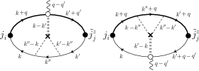
Figure 1: Feynman diagrams for $\chi^{\rm skew}_{ij}$. The thick (thin) solid line represents an electron line carrying Matsubara frequency $i\varepsilon_{n}+i\omega_{\lambda}$ $(i\varepsilon_{n})$. The dotted line (double dotted line with an open circle) represents potential (spin-orbit) scattering $V_{\rm imp}$ ($\tilde{H}_{\rm so}$) by impurities. The wavy line represents the rotation matrix ${\cal R}^{\alpha\beta}$.

We are interested in slowly varying magnetization compared with the characteristic time and length scales of electrons, and put ${\bm{q}},{\bm{q}}^{\prime}=0$ in the correlation function $\chi^{\rm skew}_{ij}$ related to the electrons. After some calculations, we obtain

$$\hskip-22.76219pt\chi^{{\rm skew}}_{ij}({\bm{q}},{\bm{q}}^{\prime},i\omega_{\lambda})=i\lambda_{\rm so}\frac{4e}{9\hbar}n_{\rm imp}^{\phantom{\dagger}}u^{3}\varepsilon_{ij\alpha}n^{\alpha}_{{\bm{q}}-{\bm{q}}^{\prime}}$$

$$\hskip-8.53581pt\times\frac{1}{\beta}\sum_{n,\sigma}\left(\sum_{{\bm{k}}}\varepsilon_{{\bm{k}}}G^{+}_{{\bm{k}}\sigma}G_{{\bm{k}}\sigma}\right)^{2}\sum_{{\bm{k}}^{\prime}}(G^{+}_{{\bm{k}}^{\prime}\sigma}-G_{{\bm{k}}^{\prime}\sigma}),$$ (17)

where $n^{\alpha}_{{\bm{q}}}$ is the Fourier component of the unit vector $n^{\alpha}({\bm{r}})$. The impurity-averaged Green’s functions are given by $G_{{\bm{k}}\sigma}(z)=(z-\xi_{{\bm{k}}\sigma}+i\gamma_{\sigma}{\rm sgn}({\rm Im}z))^{-1}$, where $\xi_{{\bm{k}}\sigma}=\varepsilon_{{\bm{k}}}-\varepsilon_{{\rm F}\sigma}$, $\varepsilon_{{\bm{k}}}=\displaystyle\frac{\hbar^{2}{\bm{k}}^{2}}{2m}$ and $\gamma_{\sigma}=\displaystyle\frac{\hbar}{2\tau_{\sigma}}$, and we put $G^{+}_{{\bm{k}}\sigma}=G_{{\bm{k}}\sigma}(i\varepsilon_{n}+i\omega_{\lambda})$ and $G_{{\bm{k}}\sigma}=G_{{\bm{k}}\sigma}(i\varepsilon_{n})$. After the analytic continuation, $i\omega_{\lambda}\to\omega+i0$, we obtain

$$\chi^{{\rm skew}}_{ij}({\bm{q}},{\bm{q}}^{\prime},\omega)=-i\omega\frac{\hbar}{e}\sigma^{\rm skew}_{\rm SH}\varepsilon_{ij\alpha}n^{\alpha}_{{\bm{q}}-{\bm{q}}^{\prime}},$$ (18)

up to ${\cal O}(\omega)$. Here we have put $\sigma^{\rm skew}_{\rm SH}=\sigma^{\rm skew}_{\uparrow}+\sigma^{\rm skew}_{\downarrow}$ with

$$\sigma^{\rm skew}_{\uparrow\,(\downarrow)}=\lambda_{\rm so}u\,\frac{2\pi e^{2}}{\hbar^{2}}(n^{\rm el}_{\uparrow\,(\downarrow)})^{2}\tau_{\uparrow\,(\downarrow)},$$ (19)

which explicitly depends on the impurity potential $u$ and the relaxation time $\tau_{\sigma}$.

Side-jump process: In the lowest order in $\lambda_{\rm so}$, the first contribution to ${\chi}^{{\rm side}}_{ij}$ comes from the second order impurity scattering (shown in Fig. 2), and is given by

$$\hskip-28.45274pt\chi^{{\rm side}}_{ij}({\bm{q}},{\bm{q}}^{\prime},i\omega_{\lambda})=i\lambda_{\rm so}\frac{4e}{3\hbar}n_{\rm imp}^{\phantom{}}u^{2}\varepsilon_{ij\alpha}n^{\alpha}_{{\bm{q}}-{\bm{q}}^{\prime}}$$ (20)

$$\times \frac{1}{\beta}\sum_{n}\sum_{{\bm{k}},{\bm{k}}^{\prime},\sigma}\varepsilon_{{\bm{k}}}G^{+}_{{\bm{k}}\sigma}G_{{\bm{k}}\sigma}(G^{+}_{{\bm{k}}^{\prime}\sigma}-G_{{\bm{k}}^{\prime}\sigma}).$$

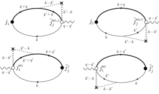
Figure 2: Feynman diagrams for $\chi^{\rm side}_{ij}$. The meaning of the diagrams is the same as Fig.1.

After the analytic continuation, $i\omega_{\lambda}\to\omega+i0$, we obtain

$$\chi^{{\rm side}}_{ij}({\bm{q}},{\bm{q}}^{\prime},\omega)=-i\omega\frac{\hbar}{e}\sigma^{\rm side}_{\rm SH}\varepsilon_{ij\alpha}n^{\alpha}_{{\bm{q}}-{\bm{q}}^{\prime}},$$ (21)

up to ${\cal O}(\omega)$. Here $\sigma^{\rm side}_{\rm SH}=\sigma^{\rm side}_{\uparrow}+\sigma^{\rm side}_{\downarrow}$, with

$$\sigma^{\rm side}_{\uparrow\,(\downarrow)}=\lambda_{\rm so}\frac{2e^{2}}{\hbar}n^{\rm el}_{\uparrow\,(\downarrow)},$$ (22)

being independent of the relaxation time.

Combining Eqs. (18) and (21), we obtain the Hall current as

$$\mathcal{J}^{\rm H}_{i}({\bm{r}},t) = \sigma_{\rm SH}\varepsilon_{i\alpha j}n^{\alpha}({\bm{r}},t)\frac{\hbar}{e}\left(-\frac{\partial}{\partial t}A_{j}^{z}({\bm{r}},t)\right)$$ (23)

$$= \sigma_{\rm SH}({\bm{n}}\times{\bm{E}}_{\rm s})_{i},$$ (24)

where $\sigma_{\rm SH}=\sigma^{\rm skew}_{\rm SH}+\sigma^{\rm side}_{\rm SH}$ is the total spin Hall conductivity, and ${\bm{E}}_{\rm s}$ is given by (12). The Hall current $\mathcal{J}^{\rm H}$ flows in the direction perpendicular to both ${\bm{n}}$ and ${\bm{E}}_{\rm s}$. This expression is our main result. The total current is given by the sum of the diagonal current and the Hall current as Eq. (2). Equations (3) and (4) can be obtained in a similar manner.

The spin-transfer torque that the $s$-electrons exert on the localized $d$-spins is represented by $\sim{\bm{j}}_{\rm S}\cdot\nabla{\bm{n}}$ KTS06 , with ${\bm{j}}_{\rm S}=\sigma_{\rm s}{\bm{E}}$ being the diagonal spin-current density, the first term in Eq.(3). The existence of the second term of Eq. (3) suggests the existence of a spin-transfer torque due to the spin Hall current, and our result (24) of the spin Hall motive force should be the reaction to this torque. Such a study will be reported elsewhere.

The (spin) Hall resistivity is given by $\rho_{\rm SH}=\sigma_{\rm SH}/\sigma^{2}_{\rm s}\sim P^{-3}\sigma_{\rm H}/\sigma^{2}_{\rm c}$, where $\sigma_{\rm H}=\sigma_{{\rm H}\uparrow}-\sigma_{{\rm H}\downarrow}$, with $\sigma_{{\rm H}\uparrow\,(\downarrow)}=\sigma^{\rm skew}_{\uparrow\,(\downarrow)}+\sigma^{\rm side}_{\uparrow\,(\downarrow)}$, is known as the extrinsic anomalous Hall conductivity DCB01 . For a typical value of $P\sim 0.5$, $\rho_{\rm SH}$ in the present case is one order of magnitudes larger than that of the conventional AHE.

DW oscillation: Let us apply the result (24) to a magnetic field driven domain wall (DW) oscillation in a ferromagnetic nanowire. We consider a Hall device, as shown in Fig. 3, where the cross section of the wire forms a square, which allows us to neglect hard axis anisotropy energy, and the one-dimensional tail-to-tail DW is positioned at $z=0$.

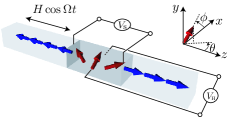
Figure 3: Schematic illustration of an experimental setup for the detection of the inverse spin Hall motive force caused by a field-driven domain wall oscillation.

When an ac magnetic field is applied along the wire $(//\hat{z})$, spins in the wall oscillate around the $z$ axis. Taking the ac field as $H_{\rm ac}(t)=H\cos\Omega t$, where $H$ is the amplitude and $\Omega$ is the frequency, and solving the Landau-Lifshitz-Gilbert equation for ${\bm{n}}$ analytically, we obtain a DW solution ${\bm{n}}=\left(\frac{\cos\phi}{\cosh\frac{z-X}{\lambda}},\frac{\sin\phi}{\cosh\frac{z-X}{\lambda}},\tanh\frac{z-X}{\lambda}\right)$, where $\phi=\frac{1}{1+\alpha^{2}}(\gamma H/\Omega)\sin\Omega t$ and $X=\alpha\lambda\phi$. Here $\gamma$ is the gyromagnetic constant, $\lambda$ is the width of the DW, and $\alpha$ is the Gilbert damping constant. Substituting this solution into Eq. (12), we obtain the spin motive force as

$$V_{\rm s}=\int_{-\infty}^{\infty}dzE_{{\rm s},z}=-\frac{\hbar}{e}\frac{\gamma H}{1+\alpha^{2}}\cos\Omega t,$$ (25)

which oscillates in time. For an open circuit condition in the lateral face of the wire, $\mathcal{J}_{x}=\mathcal{J}_{y}=0$, the Hall voltage at the DW center is obtained as

$$V_{\rm H}=\frac{\sigma_{\rm SH}}{\sigma_{\rm s}}\frac{w}{2\lambda}V_{\rm s},$$ (26)

where $w$ is the width of the wire. If we choose $w\simeq\lambda$, $\alpha=0.01$, $\gamma H=\Omega=100~{}{\rm MHz}$, and $\sigma_{\rm SH}/\sigma_{\rm s}\simeq P^{-2}\sigma_{\rm AH}/\sigma_{\rm c}\sim 1$, the amplitude of $V_{\rm H}$ is estimated as $|V_{\rm H}|\sim 31~{}{\rm nV}$, which might be detectable experimentally. For a head-to-head DW, the phase of $V_{\rm s}$ and $V_{\rm H}$ changes by $\pi$ relative to $H_{\rm ac}(t)$, and this fact may be used to discriminate the true signal.

A dc magnetic field applied in the same (easy-axis) direction can also lead to an oscillatory dynamics by the Walker’s breakdown Schryer74 , and this will produce ac signals $V_{\rm s}$ and $V_{\rm H}$ similar to the ones obtained above.

In conclusion, we have presented a microscopic theory of the AHE driven by the spin motive force due to inhomogeneous spin dynamics. It is shown that a Hall current is induced by the spin motive force in the presence of (extrinsic) spin-orbit interaction, and the corresponding Hall resistance is enhanced compared with the conventional AHE. Applying the result to the field driven domain-wall oscillation, we have shown that a Hall voltage is generated in the lateral face of the wire.

The authors would like to thank G. Tatara, Y. Nakatani and E. Saitoh for valuable discussions. We also thank Q. Niu and S. A. Yang for sending Ref. YBKXNTE08 to us before publication. This work is partially supported by a Grant-in-Aid from Monka-sho, Japan. J. S. thanks The Kurata Memorial Hitachi Science and Technology Foundation and The Sumitomo Foundation for financial support.

References

(1)
L. Berger, J. Appl. Phys. 71, 2721 (1992).
(2)
J. C. Slonczewski, J. Magn. Magn. Mater. 159, L1 (1996).
(3)
L. Berger, Phys. Rev. B 33, 1572 (1986).
(4)
A. Stern, Phys. Rev. Lett. 68, 1022 (1992).
(5)
S. E. Barnes and S. Maekawa,
Phys. Rev. Lett. 98, 246601 (2007).
(6)
W. M. Saslow,
Phys. Rev. B 76, 184434 (2007).
(7)
R. A. Duine,
Phys. Rev. B 77, 014409 (2008).
(8)
Y. Tserkovnyak and M. Mecklenburg,
Phys. Rev. B 77, 134407 (2007).
(9)
S. A. Yang el al., cond-mat:0709.1117.
(10)
S. A. Yang, G. S. D. Beach, C. Knutson, D. Xiao, Q. Niu, M. Tsoi
and J. L. Erskine, preprint.
(11)
The spin dependence of
can be made explicit by multiplying the
right-hand side of Eq. (1) by a factor
which is () for majority- (minority-) spin electrons.
(12)
E. Saitoh el al., Appl. Phys. Lett. 88, 182509 (2006).
(13)
S. O. Valenzuela and M. Tinkham, Nature 442, 176 (2006)
(14)
T, Kimura et al., Phys. Rev. Lett. 98, 156601 (2007).
(15)
T. Seki et al., Nat. Mater. 7, 125 (2008).
(16)
K. Ando et al., Phys. Rev. Lett. 101, 036601 (2008).
(17)
X. Wang et al., Phys. Rev. Lett. 97, 216602 (2006).
(18)
J. Ohe et al., Phys. Rev. Lett. 99, 266603 (2007).
(19)
A. Takeuchi and G. Tatara,
J. Phys. Soc. Jpn. 77, 074701 (2008).
(20)
J. Xiao et al., Phys. Rev. B 77, 180407(R) (2008).
(21)
J. E. Hirsch, Phys. Rev. Lett. 83, 1834 (1999).
(22)
V. K. Dugaev, et al., Phys. Rev. B 64, 104411 (2001).
(23)
V. Korenman et al., Phys. Rev. B16, 4032 (1977).
(24)
G. E. Volovik, J. Phys. C 20, L83 (1987).
(25)
G. Tatara and H. Fukuyama, Phys. Rev. Lett. 72,772 (1994).
(26)
Actually, because of the identity,
,
we need to retain terms up to the second order in .
We have, however, observed in the calculation that the second-order
terms cancel out and only the first-order terms survive
in the final expression through , Eq.(12).
(27)
The expansion parameter of the present gauge-field treatment is
and
for ,
and
and
for and TKS08 .
( and are the Fermi wavenumber and the mean free path
of electrons, and and are
characteristic length and frequency scales of the magnetization.)
(28)
G. Tatara et al., Phys. Rep. 468, 213 (2008).
(29)
J. Shibata and H. Kohno, in preparation.
(30)
W. K. Tse and S. D. Sarma, Phys. Rev. Lett. 96, 056601 (2006).
(31)
H. Kohno et al., J. Phys. Soc. Jpn. 75, 113706 (2006).
(32)
N. L. Schryer and L. R. Walker, J. Appl. Phys. 45, 5406 (1974).