Rare decays of $\Lambda_{b}\to\Lambda\gamma$ and $\Lambda_{b}\to\Lambda l^{+}l^{-}$ in universal extra dimension model

Abstract

The exclusive weak decay of $\Lambda_{b}\to\Lambda\gamma$ and $\Lambda_{b}\to\Lambda l^{+}l^{-}$ are investigated in the Applequist-Cheng-Dobrescu model, which is an extension of the standard model in presence of universal extra dimensions. Employing the transition form factors obtained in the light-cone sum rues, we analyze how the invariant mass distribution, forward-backward asymmetry and polarization asymmetry of $\Lambda$ baryon of these decay modes can be used to constrain the only one additional free parameter with respect to the standard model, namely, the radius $R$ of the extra dimension. Our results indicate that the Kaluza-Klein modes can lead to approximately 25% suppression of the branching ratio of $\Lambda_{b}\to\Lambda\gamma$, however, their contributions can bring about 10% enhancement to the decay rate of $\Lambda_{b}\to\Lambda l^{+}l^{-}$. It is shown that the zero-position of forward-backward asymmetry of $\Lambda_{b}\to\Lambda\mu^{+}\mu^{-}$ is sensitive to the compactification parameter $R$ in this scenario, while the measurement of polarizations of $\Lambda$ baryon in the $\Lambda_{b}$ decays is not suitable to provide some valuable information for the universal extra dimension model.

I Introduction

At present, the Standard Model (SM) of particle physics has been scrutinized relentlessly from its inception and held its ground over the entire breadth of its theoretical reach almost without failure. In spite of its impressive successes, the SM is not completely satisfactory as the theory of elementary particles from the view point of both aesthetics and phenomenology. It has been realized that bottom quark physics is a powerful probe of physics beyond the SM in a complementary way to the direct searches, which is crucial to identify the new physics (NP) and its properties correctly as well as understand its theoretical consequences. Rare decays involving $b\to s$ flavor changing neutral current (FCNC), which are forbidden at the tree level in the SM, can provide an ideal platform to test the SM precisely as well as bound its extensions stringently so that pave the way for the establishment of new physics beyond the SM. Wealthy experimental data on both inclusive and exclusive $b\to s$ FCNC $B$ meson decays HFAG have been accumulated at the $e^{+}e^{-}$ factories operating at the peak of $\Upsilon(4S)$, which also motivated intensive theoretical studies on these mesonic decay modes.

Unlike mesonic decays, the investigations of FCNC $b\to s$ transition for bottom baryonic decays $\Lambda_{b}\to\Lambda\gamma$ and $\Lambda_{b}\to\Lambda l^{+}l^{-}$ Mannel ; Mohanta ; Cheng ; Cheng 2 ; Huang ; Hiller:2001zj ; HLLW ; Aslam:2008hp are much behind because more degrees of freedom are involved in the bound state of baryon system at the quark level. It should be pointed out that such baryonic decays can offer the unique ground to extract the helicity structure of effective Hamiltonian for FCNC $b\to s$ transition in the SM and beyond, since the information on the handness of the quark is lost in the hadronization of meson case. Compared with the $B$ meson decays, $\Lambda_{b}$ baryon decays contain some particular observables involving the spin of $b$ quark, which are sensitive to the new physics and more easily detectable. From the viewpoint of experiment, the only drawback of bottom baryon decays is that the production rate of $\Lambda_{b}$ baryon in $b$ quark hadronization is about four times less than that of $B$ meson, hence we need more experimental data on heavy quark decays from future colliders, such as Large Hadron Colliders (LHC) at CERN, and Tevatron collider at FNAL, to perform a stringent constraint on the parameter space of available new physics models.

Among various models of physics beyond the SM, the models with extra dimensions Antoniadis:1990ew are of intensive interest, since they provide a unified framework for gravity and other interactions, which can give some hints of the hierarchy problem and a connection with string theory. Among the extra dimension models, the models of particular interests are the scenarios with universal extra dimensions (UED), which are the most democratic extra dimension model in the scene that all SM fields are allowed to propagate in the extra dimension. Above the compactification scale $1/R$, a given UED model becomes a higher dimensional field theory whose equivalent description in four dimensions consists of the SM fields, the tower of their Kaluza-Klein (KK) partners and additional tower of KK modes without corresponding SM partners. A simple scenario is represented by the Applequist-Cheng-Dobrescu (ACD) model ACD with a single compactified extra dimension, which introduces only one additional free parameter relative to the SM, i.e. $1/R$, the inverse of the compactification radius. As all particles can access the bulk, momentum along the fifth dimension, and hence the KK number is conserved in any process, which can break down to the conservation of KK-parity, defined as $(-1)^{n}$ due to the orbifold corrections.

Different bounds to the size of extra dimension have been explored in various processes already accessible at particle accelators or within the reach of future facilities. The analysis on the Tevatron run I data allows to establish the bound $1/R\geq 250-300\rm{GeV}$ Appelquist:2002wb . Analysis of the anomalous magnetic moment Agashe:2001ra ; Appelquist:2001jz and the $Z\to b\bar{b}$ vertex Oliver:2002up also gives rise to the bound $1/R\geq 300\rm{GeV}$. The conservation of KK parity implies the absence of tree level KK contributions to low energy processes taking place at scales $\mu\ll 1/R$. The fact that KK excitations can influence processes occurring at loop level also indicates that $b\to s$ FCNC transitions are extremely important for constraining the extra dimension model. For this reason, the effective Hamiltonian responsible for $b\to s$ transitions was derived in Buras:2002ej ; Buras:2003mk . $K_{L}-K_{S}$ mass difference, the parameter $\epsilon_{K}$, $B^{0}_{d,s}-\bar{B}^{0}_{d,s}$ mixing mass differences $\Delta M_{d,s}$, rare decays of $K$ and $B$ meson as well as CP-violating ratio $\epsilon^{\prime}/\epsilon$ are also comprehensively studied there. In particular, it is found that $BR(B\to X_{s}\gamma)$ allows to constrain $1/R\geq 250\rm{GeV}$ Buras:2003mk , which has been updated by a more recent analysis in combination with the NNLO values of Wilson coefficient in the SM and new experimental data to $1/R\geq 600\rm{GeV}$ at 95% C.L. Haisch:2007vb . Exclusive $B\to K^{\ast}(K_{1})l^{+}l^{-}$, $B\to K^{\ast}\nu\bar{\nu}$ and $B\to K^{\ast}\gamma$ decays of $B$ meson Colangelo together with $B_{s}\to\phi l^{+}l^{-}$ and $B_{s}\to\gamma l^{+}l^{-}$ decays of $B_{s}$ meson Mohanta:2006ae are also studied in the framework of the UED scenario.

Moreover, $\Lambda_{b}\to\Lambda\gamma$ and $\Lambda_{b}\to\nu\bar{\nu}$ decays in the UED model are further investigated in Colangelo:2007jy employing the form factors calculated in the three-point QCD sum rules (QCDSR) within the framework of heavy quark effective theory (HQET) Huang . The sensitivity of branching ratio, forward-backward asymmetry and polarization asymmetry of lepton for semileptonic decay of $\Lambda_{b}\to\Lambda l^{+}l^{-}$ to the compactification parameter $1/R$ are analyzed in Aliev:2006xd ; Aliev:2006gv using the transition form factors given by the QCDSR at length. In this work, we would like to revisit $\Lambda_{b}\to\Lambda\gamma$ and $\Lambda_{b}\to\Lambda l^{+}l^{-}$ decays in the ACD model with the form factors derived in the light-cone sum rules (LCSR) Wang:2008sm , where the effects of higher twist distribution amplitudes of $\Lambda$ baryon are included. In particular, we consider how the polarization asymmetry of $\Lambda$ baryon in $\Lambda_{b}\to\Lambda l^{+}l^{-}$ decays can be used to constrain the radius of extra dimension, which are still not available in the literature. The structure of this paper is organized as follows: After a brief introduction to the ACD model in section II, we present the effective Hamiltonian for $b\to s$ transition and parameterizations of transition form factors in section III. The dependence of branching ratio, forward-backward asymmetry and polarization asymmetry of $\Lambda$ baryon in $\Lambda_{b}\to\Lambda l^{+}l^{-}$ decays on the radius of extra dimension $R$ are given in section IV, where the sensitivity of branching fraction of $\Lambda_{b}\to\Lambda\gamma$ on the compactification parameter $R$ is also presented. The last section is devoted to the conclusion.

II Review of ACD model

In our usual universe we have 3 spatial plus 1 temporal dimensions and if an extra dimension exists and is compactified, fields living in all dimensions would manifest themselves in the $3+1$ space by the appearance of KK excitations. The most pertinent question is whether ordinary fields propagate or not in all extra dimensions. One obvious possibility is the propagation of gravity in whole ordinary plus extra dimensional universe, the “bulk”. Contrary to this there are models with UED in which all the fields propagate in all available dimensions ACD and ACD model belongs to one of UED scenarios Colangelo

This model is the minimal extension of the SM in $4+\delta$ dimensions, and in literature a simple case $\delta=1$ is considered Colangelo . The topology for this extra dimension is orbifold $S^{1}/Z_{2}$, and the coordinate $x_{5}=y$ runs from $0$ to $2\pi R$, where $R$ is the compactification radius. The KK mode expansion of the fields are determined from the boundary conditions at two fixed points $y=0$ and $y=\pi R$ on the orbifold. Under parity transformation $P_{5}:$ $y\rightarrow-y$ the fields may be even or odd. Even fields have their correspondent in the $4$-dimensional SM and their zero mode in the KK mode expansion can be interpreted as the ordinary SM field. The odd fields do not have their correspondent in the SM and therefore do not have zero mode in the KK expansion.

The salient features of the ACD model are:

• the compactification radius $R$ is the only free parameter with respect to SM

• no tree level contribution of KK modes in low energy processes (at scale $\mu\ll 1/R$) and no production of single KK excitation in ordinary particle interactions are the consequences of the conservation of KK parity.

The detailed description of ACD model is provided in Buras:2002ej ; here we summarize main features of its construction from the Ref. Colangelo .

Gauge group

As ACD model is the minimal extension of SM, therefore the gauge bosons associated with the gauge group $SU\left(2\right)_{L}\times U\left(1\right)_{Y}$ are $W_{i}^{a}\,(a=1,\,2,\,3$, $i=0$,$\,1$,$\,2$,$\,3$,$\,5)$ and $B_{i}$. The gauge couplings are $\hat{g}_{2}=g_{2}\sqrt{2\pi R}$ and $\hat{g}^{\prime}=g^{\prime}\sqrt{2\pi R}$ (the hat on the coupling constant refers to the extra dimension). The charged bosons are $W_{i}^{\pm}=\frac{1}{\sqrt{2}}\left(W_{i}^{1}\mp W_{i}^{2}\right)$ and the mixing of $W_{i}^{3}$ and $B_{i}$ gives rise to the fields $Z_{i}$ and $A_{i}$ as they do in the SM. The relations for the mixing angles are:

$$c_{W}=\cos\theta_{W}=\frac{\hat{g}_{2}}{\sqrt{\hat{g}_{2}^{2}+\hat{g}^{\prime 2}}},\qquad s_{W}=\sin\theta_{W}=\frac{\hat{g}^{\prime}}{\sqrt{\hat{g}_{2}^{2}+\hat{g}^{\prime 2}}}.$$ (1)

The Weinberg angle remains the same as in the SM, due to the relationship between five and four dimensional constants. The gluons which are the gauge bosons associated to $SU\left(3\right)_{C}$ are $G_{i}^{a}\left(x,y\right)(a=1,\ldots,8)$.

Higgs sector and mixing between Higgs fields and gauge bosons

The Higgs doublet can be written as:

$$\phi=\left(\begin{array}[]{l}\hskip 22.76228pti\chi^{+}\\ \frac{1}{\sqrt{2}}\left(\psi-i\chi^{3}\right)\end{array}\right)$$ (2)

with $\chi^{\pm}=\frac{1}{\sqrt{2}}\left(\chi^{1}\mp\chi^{2}\right)$. Now only field $\psi$ has a zero mode, and we assign vacuum expectation value $\hat{v}$ to such mode, so that $\psi\rightarrow\hat{v}+H$. $H$ is the SM Higgs field, and the relation between expectation values in five and four dimension is: $\hat{v}=v/\sqrt{2\pi R}$.

The Goldstone fields $G_{\left(n\right)}^{0}$, $G_{\left(n\right)}^{\pm}$ arise due to the mixing of charged $W_{5\left(n\right)}^{\pm}$ and $\chi_{\left(n\right)}^{\pm}$ , as well as neutral fields $Z_{5\left(n\right)}$. These Goldstone modes are then used to give masses to the $W_{\left(n\right)}^{\pm\mu}$ and $Z_{\left(n\right)}^{\mu}$, and $a_{\left(n\right)}^{0}$, $a_{\left(n\right)}^{\pm}$, new physical scalars.

Yukawa terms

In SM, Yukawa coupling of the Higgs field to the fermion provides the fermion mass terms. The diagonalization of such terms leads to the introduction of the CKM matrix. In order to have chiral fermions in ACD model, the left and right-handed components of the given spinor cannot be simultaneously even under $P_{5}$. This makes the ACD model to be the minimal flavor violation model, since there are no new operators beyond those present in the SM and no new phases beyond the CKM phase. The unitarity triangle remains the same as in SM Buras:2002ej . In order to have 4D mass eigenstates of higher KK levels, a further mixing is introduced among the left-handed doublet and right-handed singlet of each flavor $f$. The mixing angle is $\tan\left(2\alpha_{f\left(n\right)}\right)=\frac{m_{f}}{n/R}\left(n\geq 1\right)$ giving mass $m_{f\left(n\right)}=\sqrt{m_{f}^{2}+\frac{n^{2}}{R^{2}}}$, so that it is negligible for all flavors except the top Colangelo .

Integrating over the fifth-dimension $y$, one can gain the four-dimensional Lagrangian

$$\mathcal{L}_{4}\left(x\right)=\int_{0}^{2\pi R}\mathcal{L}_{5}\left(x,y\right)dy$$ (3)

which describes zero modes corresponding to the SM fields and their massive KK excitations together with KK excitations without zero modes which do not corresponds to any field in SM. The Feynman rules used in the further calculation are given in Ref. Buras:2002ej .

III Effective Hamiltonian and transition form factors

III.1 Effective Hamiltonian

Integrating out the particles including top quark, $W^{\pm}$ and $Z$ bosons above scale $\mu=O(m_{b})$ , we arrive at the effective Hamiltonian responsible for the $b\to sl^{+}l^{-}$ transition in the SM Buchalla:1995vs

$$H_{eff}(b\to sl^{+}l^{-}) = -\frac{G_{F}}{2\sqrt{2}}V_{tb}V_{ts}^{*}\bigg{[}{\sum\limits_{i=1}^{6}}C_{i}({\mu})Q_{i}({\mu})+C_{7\gamma}(\mu)Q_{7\gamma}(\mu)+C_{8G}(\mu)Q_{8G}(\mu)$$ (4)

$$+C_{9}(\mu)Q_{9}(\mu)+C_{10}(\mu)Q_{10}(\mu)\bigg{]},$$

where we have neglected the terms proportional to $V_{ub}V_{us}^{*}$ on account of $|V_{ub}V_{us}^{*}/V_{tb}V_{ts}^{*}|<0.02$. The complete list of the operators can be given by

• current–current (tree) operators

  $$Q^{u}_{1}=({\bar{s}}_{\alpha}c_{\beta})_{V-A}({\bar{c}}_{\beta}b_{\alpha})_{V-A},\ \ \ \ \ \ \ \ \ Q^{u}_{2}=({\bar{s}}_{\alpha}c_{\alpha})_{V-A}({\bar{c}}_{\beta}b_{\beta})_{V-A},$$ (5)

• QCD penguin operators

  $$Q_{3}=({\bar{s}}_{\alpha}b_{\alpha})_{V-A}\sum\limits_{q}({\bar{q}}_{\beta}q_{\beta})_{V-A},\ \ \ \ \ \ \ \ \ Q_{4}=({\bar{s}}_{\beta}b_{\alpha})_{V-A}\sum\limits_{q}({\bar{q}}_{\alpha}q_{\beta})_{V-A},$$ (6)

  $$\!\!\!\!\!\!\!\!\!\!\!\!\!\!\!\!\!\!\!\!\!\!\!\!Q_{5}=({\bar{s}}_{\alpha}b_{\alpha})_{V-A}\sum\limits_{q}({\bar{q}}_{\beta}q_{\beta})_{V+A},\ \ \ \ \ \ \ \ \ Q_{6}=({\bar{s}}_{\beta}b_{\alpha})_{V-A}\sum\limits_{q}({\bar{q}}_{\alpha}q_{\beta})_{V+A},$$ (7)

• magnetic penguin operators

  $$Q_{7\gamma}={e\over 8\pi^{2}}\bar{s}_{\alpha}\sigma^{\mu\nu}(m_{b}R+m_{s}L)b_{\alpha}\,F_{\mu\nu},\ \ \ \ Q_{8G}={g\over 8\pi^{2}}\bar{s}_{\alpha}\sigma^{\mu\nu}(m_{b}R+m_{s}L)T^{a}_{\alpha\beta}b_{\beta}\,G^{a}_{\mu\nu},$$ (8)

• semi-leptonic operators

  $$Q_{9V}=({\bar{s}}_{\alpha}b_{\alpha})_{V-A}({\bar{e}}e)_{V},\ \ \ \ Q_{10A}=({\bar{s}}_{\alpha}b_{\alpha})_{V-A}({\bar{e}}e)_{A},$$ (9)

where $\alpha$ and $\beta$ are the color indices, $R(L)=1\pm\gamma_{5},\sigma_{\mu\nu}={i\over 2}[\gamma_{\mu},\gamma_{\nu}]$, $e$ and $g$ are the coupling constant of electromagnetic and strong interactions, respectively; and $q$ are the active quarks at the scale $\mu=O(m_{b})$, i.e. $q=(u,d,s,c,b)$. The left handed current is defined as $({\bar{q}}_{\alpha}q_{\beta})_{V-A}={\bar{q}}_{\alpha}\gamma_{\nu}(1-\gamma_{5})q_{\beta}$ and the corresponding right handed current is $({\bar{q}}_{\alpha}q_{\beta})_{V+A}={\bar{q}}_{\alpha}\gamma_{\nu}(1+\gamma_{5})q_{\beta}$.

In terms of the Hamiltonian given in Eq. (4), we can derive the free quark decay amplitude for $b\to sl^{+}l^{-}$ process as

$$M(b\to sl^{+}l^{-}) = \frac{G_{F}}{2\sqrt{2}}V_{tb}V_{ts}^{*}{\alpha_{em}\over\pi}\bigg{\{}-{2i\over q^{2}}C_{7}(\mu)\bar{s}\sigma_{\mu\nu}q^{\nu}(m_{b}R+m_{s}L)b\bar{l}\gamma^{\mu}l$$ (10)

$$+C_{9}(\mu)\bar{s}\gamma_{\mu}Lb\bar{l}\gamma^{\mu}l+C_{10}\bar{s}\gamma_{\mu}Lb\bar{l}\gamma^{\mu}\gamma_{5}l\bigg{\}}.$$

Similarly, the free quark decay amplitude for $b\to s\gamma$ can be written as

$$M(b\to s\gamma) = \frac{G_{F}}{2\sqrt{2}}V_{tb}V_{ts}^{*}{e\over 4\pi^{2}}C_{7}(\mu)\bar{s}\sigma_{\mu\nu}q^{\nu}(m_{b}R+m_{s}L)bF^{\mu\nu}.$$ (11)

No operators other than those collected in Eq. (4) are found in the ACD model, therefore the effects of KK contributions are implemented by modifying the Wilson coefficients that now depend on the additional ACD parameter, the compactification radius; if we neglect the contributions of scalar fields, which are indeed very small. Since the KK states become more and more massive with large value of $1/R$, which can decouple from the low-energy theory, hence the SM phenomenology should be recovered in the limit $1/R\to+\infty$. It also needs to emphasize that we do not include the long-distance contributions from four-quark operators near the $c\bar{c}$ resonance, which can be experimentally removed applying appropriate kinematical cuts in the neighborhood of resonance region. Besides, the QCD penguin operators are also neglected due to their small Wilson coefficients compared to the others. Therefore, we only need to specify the Wilson coefficients $C_{7}$, $C_{9}$ and $C_{10}$, which have been given in Buras:2003mk . It is found that the impact of the KK states results in the enhancement of $C_{10}$ and the suppression of $C_{7}$.

As a general expression, the Wilson coefficients are represented by functions $F(x_{t},1/R)$ generalizing the SM analogues $F_{0}(x_{t})$:

$$F(x_{t}.1/R)=F_{0}(x_{t})+\sum_{n=1}^{\infty}F_{n}(x_{t},x_{n}),$$ (12)

where $x_{n}={m_{n}^{2}\over m_{W}^{2}}$ and $m_{n}={n\over R}$. A remarkable feature is that the sum over the KK contributions in Eq. (12) is finite at leading order in all cases as a result of a generalized GIM mechanism Buras:2002ej . The relevant functions are the following: $C(x_{t},1/R)$ from $Z^{0}$ penguins; $D(x_{t},1/R)$ from $\gamma$ penguins; $E(x_{t},1/R)$ from gluon penguins; $D^{\prime}(x_{t},1/R)$ from $\gamma$ magnetic penguins; $E^{\prime}(x_{t},1/R)$ from chromomagnetic penguins. They can be found in Buras:2002ej ; Buras:2003mk ; Colangelo and are collected as below.

$\bullet C_{7}$

Here one defines an effective coefficient $C_{7}^{(0)eff}$ which is renormalization scheme independent Buras:1993xp :

$$C_{7}^{(0)eff}(\mu_{b})=\eta^{\frac{16}{23}}C_{7}^{(0)}(\mu_{w})+\frac{8}{3}(\eta^{\frac{14}{23}}-\eta^{\frac{16}{23}})C_{8}^{(0)}(\mu_{w})+C_{2}^{(0)}(\mu_{w})\sum_{i=1}^{8}h_{i}\eta^{\alpha_{i}},$$ (13)

where $\eta=\frac{\alpha_{s}(\mu_{w})}{\alpha_{s}(\mu_{b})},$ and

$$C_{2}^{(0)}(\mu_{w})=1,\text{ }C_{7}^{(0)}(\mu_{w})=-\frac{1}{2}D^{\prime}(x_{t},\frac{1}{R}),\text{ }C_{8}^{(0)}(\mu_{w})=-\frac{1}{2}E^{\prime}(x_{t},\frac{1}{R});$$ (14)

the superscript $(0)$ stays for leading logarithm approximation. The involved parameters in Eq. (13) are grouped as

$$\alpha_{1} = \frac{14}{23}\text{ \quad}\alpha_{2}=\frac{16}{23}\text{ \quad}\alpha_{3}=\frac{6}{23}\text{ \quad}\alpha_{4}=-\frac{12}{23}$$

$$\alpha_{5} = 0.4086\text{ \quad}\alpha_{6}=-0.4230\text{ \quad}\alpha_{7}=-0.8994\text{ \quad}\alpha_{8}=-0.1456$$

$$h_{1} = 2.996\text{ \quad}h_{2}=-1.0880\text{ \quad}h_{3}=-\frac{3}{7}\text{ \quad}h_{4}=-\frac{1}{14}$$

$$h_{5} = -0.649\text{ \quad}h_{6}=-0.0380\text{ \quad}h_{7}=-0.0185\text{ \quad}h_{8}=-0.0057.$$ (15)

The functions $D^{\prime}$ and $E^{\prime}$ are determined by Eq. (15) with

$$D_{0}^{\prime}(x_{t})=-\frac{(8x_{t}^{3}+5x_{t}^{2}-7x_{t})}{12(1-x_{t})^{3}}+\frac{x_{t}^{2}(2-3x_{t})}{2(1-x_{t})^{4}}\ln x_{t},$$ (16)

$$E_{0}^{\prime}(x_{t})=-\frac{x_{t}(x_{t}^{2}-5x_{t}-2)}{4(1-x_{t})^{3}}+\frac{3x_{t}^{2}}{2(1-x_{t})^{4}}\ln x_{t},$$ (17)

$$D_{n}^{\prime}(x_{t},x_{n}) = \frac{x_{t}(-37+44x_{t}+17x_{t}^{2}+6x_{n}^{2}(10-9x_{t}+3x_{t}^{2})-3x_{n}(21-54x_{t}+17x_{t}^{2}))}{36(x_{t}-1)^{3}}$$

$$+\frac{x_{n}(2-7x_{n}+3x_{n}^{2})}{6}\ln\frac{x_{n}}{1+x_{n}}$$

$$-\frac{(-2+x_{n}+3x_{t})(x_{t}+3x_{t}^{2}+x_{n}^{2}(3+x_{t})-x_{n})(1+(-10+x_{t})x_{t}))}{6(x_{t}-1)^{4}}\ln\frac{x_{n}+x_{t}}{1+x_{n}},$$

$$E_{n}^{\prime}(x_{t},x_{n}) = \frac{x_{t}(-17-8x_{t}+x_{t}^{2}+3x_{n}(21-6x_{t}+x_{t}^{2})-6x_{n}^{2}(10-9x_{t}+3x_{t}^{2}))}{12(x_{t}-1)^{3}}$$ (19)

$$+-\frac{1}{2}x_{n}(1+x_{n})(-1+3x_{n})\ln\frac{x_{n}}{1+x_{n}}$$

$$+\frac{(1+x_{n})(x_{t}+3x_{t}^{2}+x_{n}^{2}(3+x_{t})-x_{n}(1+(-10+x_{t})x_{t}))}{2(x_{t}-1)^{4}}\ln\frac{x_{n}+x_{t}}{1+x_{n}}.$$

Following Buras:2002ej , one can obtain the expressions for the sum over $n$ as

$$\sum_{n=1}^{\infty}D_{n}^{\prime}(x_{t},x_{n}) = -\frac{x_{t}(-37+x_{t}(44+17x_{t}))}{72(x_{t}-1)^{3}}$$ (20)

$$+\frac{\pi M_{w}R}{2}[\int_{0}^{1}dy\frac{2y^{\frac{1}{2}}+7y^{\frac{3}{2}}+3y^{\frac{5}{2}}}{6}]\coth(\pi M_{w}R\sqrt{y})$$

$$+\frac{(-2+x_{t})x_{t}(1+3x_{t})}{6(x_{t}-1)^{4}}J(R,-\frac{1}{2})$$

$$-\frac{1}{6(x_{t}-1)^{4}}[x_{t}(1+3x_{t})-(-2+3x_{t})(1+(-10+x_{t})x_{t})]J(R,\frac{1}{2})$$

$$+\frac{1}{6(x_{t}-1)^{4}}[(-2+3x_{t})(3+x_{t})-(1+(-10+x_{t})x_{t})]J(R,\frac{3}{2})$$

$$-\frac{(3+x_{t})}{6(x_{t}-1)^{4}}J(R,\frac{5}{2})],$$

$$\sum_{n=1}^{\infty}E_{n}^{\prime}(x_{t},x_{n}) = -\frac{x_{t}(-17+(-8+x_{t})x_{t})}{24(x_{t}-1)^{3}}$$ (21)

$$+\frac{\pi M_{w}R}{2}[\int_{0}^{1}dy(y^{\frac{1}{2}}+2y^{\frac{3}{2}}-3y^{\frac{5}{2}})\coth(\pi M_{w}R\sqrt{y})]$$

$$-\frac{x_{t}(1+3x_{t})}{(x_{t}-1)^{4}}J(R,-\frac{1}{2})$$

$$+\frac{1}{(x_{t}-1)^{4}}[x_{t}(1+3x_{t})-(1+(-10+x_{t})x_{t})]J(R,\frac{1}{2})$$

$$-\frac{1}{(x_{t}-1)^{4}}[(3+x_{t})-(1+(-10+x_{t})x_{t})]J(R,\frac{3}{2})$$

$$+\frac{(3+x_{t})}{(x_{t}-1)^{4}}J(R,\frac{5}{2})],$$

where

$$J(R,\alpha)=\int_{0}^{1}dyy^{\alpha}[\coth(\pi M_{w}R\sqrt{y})-x_{t}^{1+\alpha}\coth(\pi m_{t}R\sqrt{y})].$$ (22)

$\bullet C_{9}$

In the ACD model and in the naive dimension regularization (NDR) scheme, the Wilson coefficient $C_{9}$ can be written as

$$C_{9}(\mu)=P_{0}^{NDR}+\frac{Y(x_{t},\frac{1}{R})}{\sin^{2}\theta_{W}}-4Z(x_{t},\frac{1}{R})+P_{E}E(x_{t},\frac{1}{R}),$$ (23)

where $P_{0}^{NDR}=2.60\pm 0.25$ Misiak:1992bc ; Buras:1994dj and the last term is numerically negligible. The function $Y$ and $Z$ are given by

$$Y(x_{t},\frac{1}{R}) = Y_{0}(x_{t})+\sum_{n=1}^{\infty}C_{n}(x_{t},x_{n}),$$

$$Z(x_{t},\frac{1}{R}) = Z_{0}(x_{t})+\sum_{n=1}^{\infty}C_{n}(x_{t},x_{n}),$$ (24)

where $Y_{0}(x_{t})$, $Z_{0}(x_{t})$ and $C_{n}(x_{t},x_{n})$ are

$$Y_{0}(x_{t}) = \frac{x_{t}}{8}[\frac{x_{t}-4}{x_{t}-1}+\frac{3x_{t}}{(x_{t}-1)^{2}}\ln x_{t}],$$

$$Z_{0}(x_{t}) = \frac{18x_{t}^{4}-163x_{t}^{3}+259x_{t}^{2}-108x_{t}}{144(x_{t}-1)^{3}}$$

$$+[\frac{32x_{t}^{4}-38x_{t}^{3}+15x_{t}^{2}-18x_{t}}{72(x_{t}-1)^{4}}-\frac{1}{9}]\ln x_{t},$$

$$C_{n}(x_{t},x_{n}) = \frac{x_{t}}{8(x_{t}-1)^{2}}[x_{t}^{2}-8x_{t}+7+(3+3x_{t}+7x_{n}-x_{t}x_{n})\ln\frac{x_{t}+x_{n}}{1+x_{n}}].$$ (25)

The sum of $C_{n}(x_{t},x_{n})$ over $n$ is computed as

$$\sum_{n=1}^{\infty}C_{n}(x_{t},x_{n})=\frac{x_{t}(7-x_{t})}{16(x_{t}-1)}-\frac{\pi M_{w}Rx_{t}}{16(x_{t}-1)^{2}}[3(1+x_{t})J(R,-\frac{1}{2})+(x_{t}-7)J(R,\frac{1}{2})].$$ (26)

$\bullet C_{10}$

$C_{10}$ is $\mu$ independent and is given by

$$C_{10}=-\frac{Y(x_{t},\frac{1}{R})}{\sin^{2}\theta_{w}}.$$ (27)

The renormalization scale is fixed at $\mu=\mu_{b}\simeq 5$ GeV.

III.2 Parameterizations of hadronic matrix element

With the free quark decay amplitude available, we can proceed to calculate the decay amplitudes for $\Lambda_{b}\to\Lambda\gamma$ and $\Lambda_{b}\to\Lambda l^{+}l^{-}$ at hadron level, which can be obtained by sandwiching the free quark amplitudes between the initial and final baryon states in the spirit of factorization assumption. Consequently, the following four hadronic matrix elements

$$\langle\Lambda(P)|\bar{s}\gamma_{\mu}b|\Lambda_{b}(P+q)\rangle \,\,\,\langle\Lambda(P)|\bar{s}\gamma_{\mu}\gamma_{5}b|\Lambda_{b}(P+q)\rangle,$$ ,

$$\langle\Lambda(P)|\bar{s}\sigma_{\mu\nu}b|\Lambda_{b}(P+q)\rangle \,\,\,\langle\Lambda(P)|\bar{s}\sigma_{\mu\nu}\gamma_{5}b|\Lambda_{b}(P+q)\rangle,$$ , (28)

need to be computed as can be observed from Eq. (4). Generally, the above four matrix elements can be parameterized in terms of a series of form factors as c.q. geng 4 ; Aliev 1 ; Aliev 2 ; Aliev 3 ; Aliev 4

$$\langle\Lambda(P)|\bar{s}\gamma_{\mu}b|\Lambda_{b}(P+q)\rangle = \overline{\Lambda}(P)(g_{1}\gamma_{\mu}+g_{2}i\sigma_{\mu\nu}q^{\nu}+g_{3}q_{\mu})\Lambda_{b}(P+q),\,\,$$ (29)

$$\langle\Lambda(P)|\bar{s}\gamma_{\mu}\gamma_{5}b|\Lambda_{b}(P+q)\rangle = \overline{\Lambda}(P)(G_{1}\gamma_{\mu}+G_{2}i\sigma_{\mu\nu}q^{\nu}+G_{3}q_{\mu})\gamma_{5}\Lambda_{b}(P+q),\,\,$$ (30)

$$\langle\Lambda(P)|\bar{s}i\sigma_{\mu\nu}q^{\nu}b|\Lambda_{b}(P+q)\rangle = \overline{\Lambda}(P)(f_{1}\gamma_{\mu}+f_{2}i\sigma_{\mu\nu}q^{\nu}+f_{3}q_{\mu})\Lambda_{b}(P+q),\,\,$$ (31)

$$\langle\Lambda(P)|\bar{s}i\sigma_{\mu\nu}\gamma_{5}q^{\nu}b|\Lambda_{b}(P+q)\rangle = \overline{\Lambda}(P)(F_{1}\gamma_{\mu}+F_{2}i\sigma_{\mu\nu}q^{\nu}+F_{3}q_{\mu})\gamma_{5}\Lambda_{b}(P+q),$$ (32)

where all the form factors $g_{i}$, $G_{i}$, $f_{i}$ and $F_{i}$ are functions of the square of momentum transfer $q^{2}$.

It should be emphasized that the form factors $f_{3}$ and $F_{3}$ do not contribute to the decay amplitude of $\Lambda_{b}\to\Lambda+l^{+}l^{-}$ due to the conservation of vector current, namely $q^{\mu}\bar{l}\gamma_{\mu}l=0$. Concentrating on the radiative decay of $\Lambda_{b}\to\Lambda\gamma$, we then observe that the matrix element of magnetic penguin operators can be simplified as

$$\langle\Lambda(P)|\bar{s}i\sigma_{\mu\nu}q^{\nu}b|\Lambda_{b}(P+q)\rangle = f_{2}(0)\overline{\Lambda}(P)i\sigma_{\mu\nu}q^{\nu}\Lambda_{b}(P+q),\,\,$$ (33)

$$\langle\Lambda(P)|\bar{s}i\sigma_{\mu\nu}\gamma_{5}q^{\nu}b|\Lambda_{b}(P+q)\rangle = F_{2}(0)\overline{\Lambda}(P)i\sigma_{\mu\nu}\gamma_{5}q^{\nu}\Lambda_{b}(P+q).$$ (34)

For the completeness, we also present the parameterizations of matrix elements involving the scalar $\bar{s}b$ and pseudo-scalar $\bar{s}\gamma_{5}b$ currents, which can be obtained from the Eqs. (29) and (30) by contracting both sides to the four-momentum $q^{\mu}$

$$\langle\Lambda(P)|\bar{s}b|\Lambda_{b}(P+q)\rangle = {1\over m_{b}+m_{s}}\overline{\Lambda}(P)[g_{1}(m_{\Lambda_{b}}-m_{\Lambda})+g_{3}q^{2}]\Lambda_{b}(P+q),\,\,$$ (35)

$$\langle\Lambda(P)|\bar{s}\gamma_{5}b|\Lambda_{b}(P+q)\rangle = {1\over m_{b}-m_{s}}\overline{\Lambda}(P)[G_{1}(m_{\Lambda_{b}}+m_{\Lambda})-G_{3}q^{2}]\gamma_{5}\Lambda_{b}(P+q).$$ (36)

IV Branching ratio, forward-backward asymmetry and polarization asymmetry

Now, we are going to analyze the sensitivity of the branching ratio, forward-backward asymmetry and polarization asymmetry of $\Lambda$ baryon on the radius of extra dimension $R$. To this purpose, we firstly list the input parameters used in this paper in Table 1.

Table 1: Values of input parameters used in our numerical analysis

$G_{F}=1.166\times 10^{-2}$ GeV-2	$\left|V_{ts}\right|=41.61_{-0.80}^{+0.10}\times 10^{-3}$
$\left|{V_{tb}}\right|=0.9991$	$m_{b}=\left(4.68\pm 0.03\right)$ GeV
$m_{c}\left(m_{c}\right)=1.275_{-0.015}^{+0.015}$ GeV	$m_{s}\left(1\text{ GeV}\right)=\left(142\pm 28\right)$ MeV
$m_{\Lambda_{b}}=5.62$ GeV	$m_{\Lambda}=1.12$ GeV
$m_{\mu}=0.106{\rm GeV}$	$m_{\tau}=1.777{\rm GeV}$

In addition, we also collect here the form factors calculated in the Ref. Wang:2008sm , where the effects of higher twist distribution amplitudes of $\Lambda$ baryon are included in the sum rules of transition form factors. Specifically, the dependence of form factors on the transfer momentum are parameterized as Wang:2008sm

$$\xi_{i}(q^{2})={\frac{\xi_{i}(0)}{1-a_{1}q^{2}/m_{\Lambda_{b}}^{2}+a_{2}q^{4}/m_{\Lambda_{b}}^{4}}},$$ (37)

where $\xi_{i}$ denotes the form factors $f_{2}$ and $g_{2}$. The numbers of parameters $\xi_{i}(0),\,\,a_{1},\,\,a_{2}$ have been collected in Table LABEL:di-fit.

Table 2: Numerical results for the form factors $f_{2}(0)$, $g_{2}(0)$ and parameters $a_{1}$ and $a_{2}$ involved in the double-pole fit of Eq. (37) for both twist-3 and twist-6 sum rules with $M_{B}^{2}\in[3.0,6.0]~{}\mbox{GeV}^{2}$, $s_{0}=39\pm 1~{}\mbox{GeV}^{2}$.

parameter	COZ	FZOZ	QCDSR	twist-3	up to twist-6
$f_{2}(0)$	$0.74^{+0.06}_{-0.06}$	$0.87^{+0.07}_{-0.07}$	$0.45$	$0.14^{+0.02}_{-0.01}$	$0.15^{+0.02}_{-0.02}$
$a_{1}$	$2.01^{+0.17}_{-0.10}$	$2.08^{+0.15}_{-0.09}$	0.57	$2.91^{+0.10}_{-0.07}$	$2.94^{+0.11}_{-0.06}$
$a_{2}$	$1.32^{+0.14}_{-0.08}$	$1.41^{+0.11}_{-0.08}$	$-0.18$	$2.26^{+0.13}_{-0.08}$	$2.31^{+0.14}_{-0.10}$
$g_{2}(0)(10^{-2}\rm{GeV^{-1}})$	$-2.4^{+0.3}_{-0.2}$	$-2.8^{+0.4}_{-0.2}$	$-1.4$	$-0.47^{+0.06}_{-0.06}$	$1.3^{+0.2}_{-0.4}$
$a_{1}$	$2.76^{+0.16}_{-0.13}$	$2.80^{+0.16}_{-0.11}$	2.16	$3.40^{+0.06}_{-0.05}$	$2.91^{+0.12}_{-0.09}$
$a_{2}$	$2.05^{+0.23}_{-0.13}$	$2.12^{+0.21}_{-0.13}$	1.46	$2.98^{+0.09}_{-0.08}$	$2.24^{+0.17}_{-0.13}$

To the leading order in $\alpha_{s}$ and leading contributions in the infinite momentum kinematics, the other form factors can be related to these two as

$$F_{1}(q^{2}) = f_{1}(q^{2})=q^{2}g_{2}(q^{2})=q^{2}G_{2}(q^{2}),$$

$$F_{2}(q^{2}) = f_{2}(q^{2})=g_{1}(q^{2})=G_{1}(q^{2}),$$ (38)

where the form factors $F_{3}(q^{2})$ and $G_{3}(q^{2})$ are dropped out here due to their tiny contributions.

IV.1 Decay width of $\Lambda_{b}\to\Lambda+\gamma$

Making use of Eqs. (33) and (34), the decay width of $\Lambda_{b}\to\Lambda\gamma$ can be written as

$$\Gamma(\Lambda_{b}\to\Lambda\gamma)={\alpha_{em}G_{F}^{2}\over 32m_{\Lambda_{b}}^{3}\pi^{4}}|V_{tb}|^{2}|V_{ts}|^{2}|C_{7}|^{2}(1-x^{2})^{3}(m_{b}^{2}+m_{s}^{2})[f_{2}(0)]^{2}.$$ (39)

The numerical evaluation of $BR(\Lambda_{b}\to\Lambda\gamma)$ in the SM indicates that it can be as large as $(0.63-0.73)\times 10^{-5}$, hence this process is within the reach of LHC experiments. To explore the effects of KK states in this process, we present the dependence of decay rate on the compactification parameter $1/R$ in Fig. 1. As can be observed from this figure, the branching fraction is suppressed for low values of $1/R$, which is around 25% smaller for $1/R=300{\rm{GeV}}$ than that in the SM. Such kind of suppression from KK modes is reflected in the Wilson coefficient $C_{7}^{(0)eff}(\mu_{b})$, whose value at $m_{b}$ scale decreases from $-0.300$ in the SM to $-0.245$ in the ACD model Buras:2003mk . As a matter of fact, the suppression of branching fraction for $b\to s$ transition has already been found in the inclusive decay process $B\to X_{s}\gamma$ Buras:2003mk ; Agashe:2001ra .

For a comparison, we also display the result of $BR(\Lambda_{b}\to\Lambda\gamma)$ as a function of parameter $1/R$ in Fig. 1, utilizing the transition form factors calculated in the COZ and FZOZ modes for the distribution amplitudes of $\Lambda$ baryon. Up to now, only the upper bound $1.3\times 10^{-3}$ for branching ratio of $\Lambda_{b}\to\Lambda\gamma$ decay is available in experiment, so the forthcoming experimental data can not only be used to constrain the additional parameter $R$ with respect to the SM but also are helpful to discriminate existing models of distribution amplitudes for $\Lambda$ baryon.

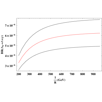
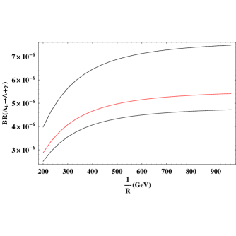
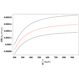
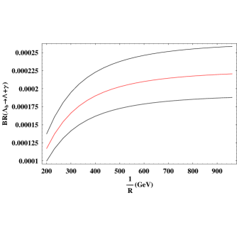
Figure 1: (Color online). Decay rate of $\Lambda_{b}\to\Lambda+\gamma$ as a function of compactification parameter $1/R$. The center line describes the case using the central values of form factors; while the other two lines correspond to the results of branching ratio when the errors in the form factors are added and subtracted from their central values. The fig. (a) and (b) denote the $BR(\Lambda_{b}\to\Lambda+\gamma)$ using the transition form factors up to twist-6 and twist-3 respectively; while fig. (c) and (d) are obtained based on the form factors calculated in the COZ and FZOZ model respectively.

IV.2 Decay width and dilepton distributions of $\Lambda_{b}\to\Lambda+l^{+}l^{-}$

The differential decay width of $\Lambda_{b}\to\Lambda l^{+}l^{-}$ in the rest frame of $\Lambda_{b}$ baryon can be written as PDG ,

$${d\Gamma({\Lambda_{b}\to\Lambda l^{+}l^{-}})\over dq^{2}}={1\over(2\pi)^{3}}{1\over 32m_{\Lambda_{b}}^{3}}\int_{u_{min}}^{u_{max}}|{\widetilde{M}}_{\Lambda_{b}\to\Lambda l^{+}l^{-}}|^{2}du,$$ (40)

where $u=(p_{\Lambda}+p_{l^{-}})^{2}$ and $q^{2}=(p_{l^{+}}+p_{l^{-}})^{2}$; $p_{\Lambda}$, $p_{l^{+}}$ and $p_{l^{-}}$ are the four-momenta vectors of $\Lambda$, $l^{+}$ and $l^{-}$ respectively. ${\widetilde{M}}_{\Lambda_{b}\to\Lambda l^{+}l^{-}}$ is the decay amplitude after integrating over the angle between the $l^{-}$ and $\Lambda$ baryon. The upper and lower limits of $u$ are given by

$$u_{max} = (E^{\ast}_{\Lambda}+E^{\ast}_{l})^{2}-(\sqrt{E_{\Lambda}^{\ast 2}-m_{\Lambda}^{2}}-\sqrt{E_{l}^{\ast 2}-m_{l}^{2}})^{2},$$

$$u_{min} = (E^{\ast}_{\Lambda}+E^{\ast}_{l})^{2}-(\sqrt{E_{\Lambda}^{\ast 2}-m_{\Lambda}^{2}}+\sqrt{E_{l}^{\ast 2}-m_{l}^{2}})^{2};$$ (41)

where $E^{\ast}_{\Lambda}$ and $E^{\ast}_{l}$ are the energies of $\Lambda$ and $l^{-}$ in the rest frame of lepton pair

$$E^{\ast}_{\Lambda}={m_{\Lambda_{b}}^{2}-m_{\Lambda}^{2}-q^{2}\over 2\sqrt{q^{2}}},\hskip 28.45274ptE^{\ast}_{l}={q^{2}\over 2\sqrt{q^{2}}}.$$ (42)

The total decay rates of $\Lambda_{b}\to\Lambda l^{+}l^{-}$ ($l=\mu,\,\tau$) in the ACD model have been plotted in the Fig. 2, from which we can observe that the KK states can result in 10% enhancement with fixed $1/R=300{\rm GeV}$ compared with that in the SM. This can be easily understood since the Wilson coefficient $C_{9}$ is essentially the same as that in the SM and $C_{10}$ is significantly enhanced, which can overwhelm the suppression from $C_{7}$. The enhancement effect due to KK modes in the $b\to sl^{+}l^{-}$ transition is already found in the inclusive decay $B\to X_{s}\mu^{+}\mu^{-}$ Buras:2003mk . Furthermore, the dilepton distributions of $\Lambda_{b}\to\Lambda+l^{+}l^{-}$ are also displayed in Fig. 3, where the predictions in the SM are also included for completeness. As can be seen, the invariant mass distribution amplitude is not sensitive to the effect of extra dimension for both the muon and tauon cases.

Figure 2: Decay rate of $\Lambda_{b}\to\Lambda+l^{+}l^{-}$ ($l=\mu,\,\tau$) as a function of compactification parameter $1/R$ within the range [200,1000] GeV. The dashed (dot-dashed) lines correspond to the results of branching fractions when the errors in the form factors are added to (subtracted from) their central values.

Figure 3: Dilepton distributions of $\Lambda_{b}\to\Lambda+l^{+}l^{-}$ as a function of $q^{2}$ at two different values of $1/R$. The fig. (a) and (b) are for the muon case with $1/R=500\rm{GeV}$ and $1/R=200\rm{GeV}$ respectively; while fig. (c) and (d) are for the tauon case with $1/R=500\rm{GeV}$ and $1/R=200\rm{GeV}$ respectively. The solid lines correspond to the results obtained in the SM with the central value of form factors, the dashed (dot-dashed) lines describe the results in the ACD model when the errors in the form factors are added to (subtracted from) their central values.

IV.3 Forward-backward asymmetry of $\Lambda_{b}\to\Lambda+l^{+}l^{-}$

Following Refs. c.q. geng 4 ; b to s in theory 9 , the differential and normalized forward-backward asymmetries for the semi-leptonic decay $\Lambda_{b}\to\Lambda l^{+}l^{-}$ can be defined as

$${dA_{FB}(q^{2})\over dq^{2}}=\int_{0}^{1}dz{d^{2}\Gamma(q^{2},z)\over dq^{2}dz}-\int_{-1}^{0}dz{d^{2}\Gamma(q^{2},z)\over dq^{2}dz}.$$ (43)

and

$$A_{FB}(q^{2})={\int_{0}^{1}dz{d^{2}\Gamma(q^{2},z)\over dq^{2}dz}-\int_{-1}^{0}dz{d^{2}\Gamma(q^{2},z)\over dq^{2}dz}\over\int_{0}^{1}dz{d^{2}\Gamma(q^{2},z)\over dq^{2}dz}+\int_{-1}^{0}dz{d^{2}\Gamma(q^{2},z)\over dq^{2}dz}}.$$ (44)

Making use of the decay amplitude in Eq. (10), the differential forward-backward asymmetry for decays of $\Lambda_{b}\to\Lambda+l^{+}l^{-}$ can be calculated as

$${dA_{FB}(q^{2})\over dq^{2}}={G_{F}^{2}\alpha_{em}^{2}|V_{tb}V_{ts}^{\ast}|^{2}\over 256m_{\Lambda_{b}}^{3}\pi^{5}}\lambda(m_{\Lambda_{b}}^{2},m_{\Lambda}^{2},q^{2})(1-{4m_{l}^{2}\over q^{2}})R_{FB}(q^{2}),$$ (45)

with

$$R_{FB}(q^{2}) = 2[(m_{s}m_{\Lambda}+m_{b}m_{\Lambda_{b}})f_{2}^{2}-m_{s}(m_{\Lambda}^{2}-m_{\Lambda_{b}}^{2}+q^{2})f_{2}g_{2}+(m_{s}m_{\Lambda}-m_{b}m_{\Lambda_{b}})q^{2}g_{2}^{2}]{\rm{Re}}(C_{7}^{eff}C_{10}^{\ast})$$ (46)

$$+[(f_{2}-g_{2}m_{\Lambda})^{2}-g_{2}^{2}m_{\Lambda_{b}}^{2}]q^{2}{\rm{Re}}(C_{9}^{eff}C_{10}^{\ast}),$$

where we have retained masses for both the lepton and strange quark.

In fig. 4, we show the dependence of $A_{FB}$ on the momentum transfer $q^{2}$ at two fixed values of $1/R=200{\rm GeV}$ and $500{\rm GeV}$ as well as that in the SM for both the muon and tauon cases. As can be seen from the figure, the zero-position of forward-backward asymmetry for $\Lambda_{b}\to\Lambda+\mu^{+}\mu^{-}$ is sensitive on the compactification parameter $1/R$, which is consistent with that observed in Aliev:2006xd . For the case of $1/R=500{\rm GeV}$, the forward-backward asymmetry is quite close to that in the SM for both two cases of the final states. For this reason, experimental determination of the zero-point of $A_{FB}$ for $\Lambda_{b}\to\Lambda+\mu^{+}\mu^{-}$ can provide valuable information on the new physics effects. Similar to that in the SM, there is no zero position of forward-backward asymmetry for the case of $\Lambda_{b}\to\Lambda+\tau^{+}\tau^{-}$ in the ACD model apart from the end point regions.

Figure 4: Forward-backward asymmetry of $\Lambda_{b}\to\Lambda+l^{+}l^{-}$ ($l=\mu,\,\tau$) as a function of momentum transfer $q^{2}$ at two fixed value of $1/R$ and in the SM. The solid line represents the case in the SM; while the dashed (dot-dashed) lines correspond to the cases with the value of $1/R$ being 200 GeV and 500 GeV respectively.

IV.4 $\Lambda$ baryon polarization asymmetry of $\Lambda_{b}\to\Lambda+l^{+}l^{-}$

To study the $\Lambda$ spin polarization, one needs to express the $\Lambda$ four spin vector in terms of a unit vector $\vec{\xi}$ along the $\Lambda$ spin in its rest frame as c.q. geng 2

$$s_{0}=\frac{\vec{p}_{\Lambda}\cdot\vec{\xi}}{m_{\Lambda}},\text{ }\vec{s}=\vec{\xi}+\frac{s_{0}}{E_{\Lambda}+m_{\Lambda}}\vec{p}_{\Lambda}.$$ (47)

The unit vectors along the longitudinal, normal and transverse components of the $\Lambda$ polarization are chosen to be

$$\hat{e}_{L} = \frac{\vec{p}_{\Lambda}}{\left|\vec{p}_{\Lambda}\right|},$$ (48)

$$\hat{e}_{N} = \frac{\vec{p}_{\Lambda}\times(\vec{p}_{-}\times\vec{p}_{\Lambda})}{\left|\vec{p}_{\Lambda}\times(\vec{p}_{-}\times\vec{p}_{\Lambda})\right|},$$ (49)

$$\hat{e}_{T} = \frac{\vec{p}_{-}\times\vec{p}_{\Lambda}}{\left|\vec{p}_{-}\times\vec{p}_{\Lambda}\right|},$$ (50)

where $\vec{p}_{-}$ and $\vec{p}_{\Lambda}$ are the three-momenta of the lepton $l^{-}$ and $\Lambda$ baryon respectively in the center mass frame of $l^{+}l^{-}$ system.

The polarization asymmetries for $\Lambda$ baryon in $\Lambda_{b}\rightarrow\Lambda l^{+}l^{-}$ can be defined as

$$P_{i}^{(\mp)}(q^{2})=\frac{\frac{d\Gamma}{dq^{2}}(\vec{\xi}=\hat{e}_{i})-\frac{d\Gamma}{dq^{2}}(\vec{\xi}=-\hat{e}_{i})}{\frac{d\Gamma}{dq^{2}}(\vec{\xi}=\hat{e}_{i})+\frac{d\Gamma}{dq^{2}}(\vec{\xi}=-\hat{e}_{i})}$$ (51)

where $i=L,\;N,\;T$ and $\vec{\xi}$ is the spin direction along the $\Lambda$ baryon. The differential decay rate for polarized $\Lambda$ baryon in $\Lambda_{b}\rightarrow\Lambda l^{+}l^{-}$ decay along any spin direction $\vec{\xi}$ is related to the unpolarized decay rate (40) through the following relation

$$\frac{d\Gamma(\vec{\xi})}{dq^{2}}=\frac{1}{2}\left(\frac{d\Gamma}{dq^{2}}\right)[1+(P_{L}\vec{e}_{L}+P_{N}\vec{e}_{N}+P_{T}\vec{e}_{T})\cdot\vec{\xi}].$$ (52)

In the Fig. 5, we display the longitudinal polarization asymmetry of $\Lambda$ baryon for both the muon and tauon cases with two fixed numbers of $1/R$ in the ACD model together with that in the SM, from which one can see that the impact of extra dimension on this asymmetry is rather weak. The normal polarization asymmetry of $\Lambda$ baryon has been plotted in fig. 6, from which we can find that the effects of KK states are more important at large momentum transfer $q^{2}$ and might be distinguishable from that in the SM for the case of $1/R=200\rm{GeV}$. As for the transverse polarization asymmetry, both the ACD model and the SM can give very tiny predictions, which is almost impossible to detect in the future colliders. In short, the measurement of polarization asymmetries of $\Lambda$ baryon in $\Lambda_{b}\to\Lambda+l^{+}l^{-}$ decays is not so helpful to establish the UED models. This is much very similar to the case of single-lepton polarization as found in Ref. Aliev:2006xd .

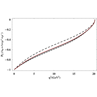
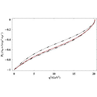
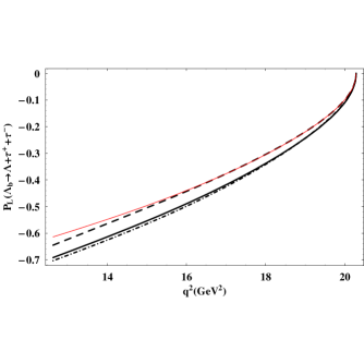
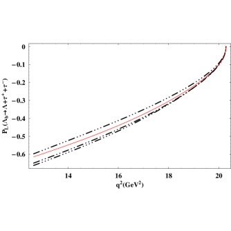
Figure 5: (Color online). Longitudinal polarization asymmetry of $\Lambda_{b}\to\Lambda+l^{+}l^{-}$ ($l=\mu,\,\tau$) as a function of momentum transfer $q^{2}$ at two fixed value of $1/R$ and in the SM. The red line represents the case in the SM;. The fig. (a) and (b) describe the muon cases with the value of $1/R$ being 200 GeV and 500 GeV respectively; while fig. (c) and (d) reflect the tauon cases with the value of $1/R$ being 200 GeV and 500 GeV.

Figure 6: Normal polarization asymmetry of $\Lambda_{b}\to\Lambda+l^{+}l^{-}$ ($l=\mu,\,\tau$) as a function of momentum transfer $q^{2}$ at two fixed value of $1/R$ and in the SM. The bold line represents the case in the SM;. The fig. (a) and (b) describe the muon cases with the value of $1/R$ being 200 GeV and 500 GeV respectively; while fig. (c) and (d) reflect the tauon cases with the value of $1/R$ being 200 GeV and 500 GeV.

V Conclusions

In this paper, we investigate the exclusive weak decay of $\Lambda_{b}\to\Lambda\gamma$ and $\Lambda_{b}\to\Lambda l^{+}l^{-}$ ($l=\mu\,\tau$) in a single universal extra dimension scenario, which is a strong contender to explore physics beyond the SM. The priority to investigate the bottom decays can be attributed to their sensitivity of the flavor structure of nature, which leads to an extremely rich phenomenology. More important, the large mass of heavy quark makes the troublesome strong interaction effects controllable within heavy quark expansion on the theoretical side, allowing for theoretical predictions of acceptable accuracy. The form factors responsible for $\Lambda_{b}\to\Lambda$ transition used in this paper are borrowed from that calculated in the LCSR approach, where the higher twist distribution amplitudes of $\Lambda$ baryon are included.

Due to the suppression of Wilson coefficient $C_{7}$ in the ACD model, we find that the branching fraction $BR(\Lambda_{b}\to\Lambda\gamma)$ is suppressed by 25% for $1/R=300{\rm{GeV}}$ compared with that in the SM, which is similar to the inclusive $B\to X_{s}\gamma$ decay Buras:2003mk . However, the contributions from KK modes can give rise to 10% enhancement for fixed value of $1/R=300{\rm{GeV}}$ as a consequence of larger number of Wilson coefficient $C_{10}$ compared with that in the SM. Besides, it is found that the zero-position of forward-backward asymmetry for $\Lambda_{b}\to\Lambda\mu^{+}\mu^{-}$ is sensitive on the radius of extra dimension $R$, which can be used to probe the new physics effectively once the experimental data are available. The longitudinal and transverse polarization asymmetries of $\Lambda$ baryon for the decays of $\Lambda_{b}\to\Lambda l^{+}l^{-}$ are found to be insensitive to the effect of extra dimension in the ACD model. For the case of large momentum transverse $q^{2}$, the normal polarization asymmetry $P_{N}(q^{2})$ of $\Lambda_{b}\to\Lambda l^{+}l^{-}$ in the UED model can be marginally distinguishable from that in the SM. Absolutely, it is also worth to extend the analysis of $\Lambda_{b}\to\Lambda$ transition presented here to the case of $\Lambda_{b}$ decays to heavier $\Lambda$- baryons (resonance), which may be another interesting field to explore the effects from extra dimensions and will be investigated in our future work.

References

- (1) The Heavy Flavor Averaging Group, arXiv:0808.1297 [hep-ex], and online update at http://www.slac.stanford.edu/xorg/hfag/ .
- (2) T. Mannel and S. Recksiegel, J. Phys. G 24 (1998) 979 [arXiv:hep-ph/9701399].
- (3) R. Mohanta, A. K. Giri, M. P. Khanna, M. Ishida and S. Ishida, Prog. Theor. Phys. 102 (1999) 645 [arXiv:hep-ph/9908291].
- (4) H. Y. Cheng, C. Y. Cheung, G. L. Lin, Y. C. Lin, T. M. Yan and H. L. Yu, Phys. Rev. D 51 (1995) 1199 [arXiv:hep-ph/9407303].
- (5) H. Y. Cheng and B. Tseng, Phys. Rev. D 53, 1457 (1996) [Erratum-ibid. D 55, 1697 (1997)] [arXiv:hep-ph/9502391].
- (6) C. S. Huang and H. G. Yan, Phys. Rev. D 59 (1999) 114022 [Erratum-ibid. D 61 (2000) 039901] [arXiv:hep-ph/9811303].
- (7) G. Hiller and A. Kagan, Phys. Rev. D 65 (2002) 074038 [arXiv:hep-ph/0108074].
- (8) X. G. He, T. Li, X. Q. Li and Y. M. Wang, Phys. Rev. D 74 (2006) 034026 [arXiv:hep-ph/0606025].
- (9) M. J. Aslam, Y. M. Wang and C. D. Lu, arXiv:0808.2113 [hep-ph].
- (10) I. Antoniadis, Phys. Lett. B 246 (1990) 377.
- (11) T. Appelquist, H. C. Cheng and B. A. Dobrescu, Phys. Rev. D 64 (2001) 035002 [arXiv:hep-ph/0012100].
- (12) T. Appelquist and H. U. Yee, Phys. Rev. D 67 (2003) 055002 [arXiv:hep-ph/0211023].
- (13) K. Agashe, N. G. Deshpande and G. H. Wu, Phys. Lett. B 511 (2001) 85 [arXiv:hep-ph/0103235].
- (14) T. Appelquist and B. A. Dobrescu, Phys. Lett. B 516 (2001) 85 [arXiv:hep-ph/0106140].
- (15) J. F. Oliver, J. Papavassiliou and A. Santamaria, Phys. Rev. D 67 (2003) 056002 [arXiv:hep-ph/0212391].
- (16) A. J. Buras, M. Spranger and A. Weiler, Nucl. Phys. B 660 (2003) 225 [arXiv:hep-ph/0212143].
- (17) A. J. Buras, A. Poschenrieder, M. Spranger and A. Weiler, Nucl. Phys. B 678 (2004) 455 [arXiv:hep-ph/0306158].
- (18) U. Haisch and A. Weiler, Phys. Rev. D 76 (2007) 034014 [arXiv:hep-ph/0703064].
- (19) P. Colangelo, F. De Fazio, R. Ferrandes and T. N. Pham, Phys. Rev. D 73 (2006) 115006 [arXiv:hep-ph/0604029]; I. Ahmed, M. A. Paracha and M. J. Aslam, Eur. Phys. J. C 54 (2008) 591 [arXiv:0802.0740 [hep-ph]]; A. Saddique, M. J. Aslam and C. D. Lu, Eur. Phys. J. C 56 (2008) 267 [arXiv:0803.0192 [hep-ph]].
- (20) R. Mohanta and A. K. Giri, Phys. Rev. D 75 (2007) 035008 [arXiv:hep-ph/0611068].
- (21) P. Colangelo, F. De Fazio, R. Ferrandes and T. N. Pham, Phys. Rev. D 77 (2008) 055019 [arXiv:0709.2817 [hep-ph]].
- (22) T. M. Aliev and M. Savci, Eur. Phys. J. C 50 (2007) 91 [arXiv:hep-ph/0606225].
- (23) T. M. Aliev, M. Savci and B. B. Sirvanli, Eur. Phys. J. C 52 (2007) 375 [arXiv:hep-ph/0608143].
- (24) Y. M. Wang, Y. Li and C. D. Lu, arXiv:0804.0648 [hep-ph].
- (25) G. Buchalla, A. J. Buras and M. E. Lautenbacher, Rev. Mod. Phys. 68 (1996) 1125 [arXiv:hep-ph/9512380].
- (26) A. J. Buras, M. Misiak, M. Munz and S. Pokorski, Nucl. Phys. B 424 (1994) 374 [arXiv:hep-ph/9311345].
- (27) M. Misiak, Nucl. Phys. B 393 (1993) 23 [Erratum-ibid. B 439 (1995) 461].
- (28) A. J. Buras and M. Munz, Phys. Rev. D 52 (1995) 186 [arXiv:hep-ph/9501281].
- (29) C. H. Chen and C. Q. Geng, Phys. Rev. D 64 (2001) 074001 [arXiv:hep-ph/0106193].
- (30) T. M. Aliev, A. Ozpineci and M. Savci, Nucl. Phys. B 649 (2003) 168 [arXiv:hep-ph/0202120].
- (31) T. M. Aliev, A. Ozpineci and M. Savci, Phys. Rev. D 67 (2003) 035007 [arXiv:hep-ph/0211447].
- (32) T. M. Aliev, V. Bashiry and M. Savci, Nucl. Phys. B 709 (2005) 115 [arXiv:hep-ph/0407217].
- (33) T. M. Aliev and M. Savci, JHEP 0605 (2006) 001 [arXiv:hep-ph/0507324].
- (34) W.M. Yao et al., J. Phys. G 33, 1 (2006).
- (35) A. Ali, T. Mannel and T. Morozumi, Phys. Lett. B273 (1991) 505.
- (36) C. H. Chen and C. Q. Geng, Phys. Rev. D 63 (2001) 114024 [arXiv:hep-ph/0101171].