QCD Cosmology from the Lattice Equation of State

Abstract

We numerically determine the time dependence of the scale factor from the lattice QCD equation of state, which can be used to define a QCD driven cosmology. We compare a lattice approach to QCD cosmology at late times with other models of the low temperature equation of state including the hadronic resonance gas model, Hagedorn model and AdS/CFT.

1 Introduction

QCD cosmology is important as the Universe exits the radiation dominated era and enters the matter dominated era, eventually evolving into the dark energy dominated era [1, 2, 3, 4, 5, 6, 7, 8, 9]. The effect of the strong interactions on cosmology was considered early on [10, 11] but the nonperturbative nature of the strong interactions at low energy limited the progress of the subject. Today with nonperturbative approaches like lattice QCD [12] and AdS/QCD [13, 14, 15] it is important to revisit the subject to see what can be said quantitatively about QCD cosmology. Also besides the time dependence of the scale factor in QCD cosmology, one can also look at the effect of recent advances on the QCD equation of state for exotic astrophysical objects like quark or strange stars [16, 17].

In this paper we consider a spatially flat Friedmann-Robertson-Walker Universe where the radius of the Universe $a(t)$, energy density $\varepsilon$, and pressure $p$ all depend on time. Conservation of the local energy-momentum tensor leads to:

$$\frac{{d(\varepsilon a^{3})}}{{dt}}=-p\frac{{d(a^{3})}}{{dt}}.$$

The Friedmann equation relates the time evolution of the Universe to energy density and is is given by:

$$3M_{P}^{2}(\frac{1}{a}\frac{{da}}{{dt}})^{2}=\varepsilon$$ (1.1)

where $M_{P}=\sqrt{1/8\pi G_{N}}$ is the reduced Planck mass. The equation of state refers to the dependence of energy density and pressure on temperature $T$. For a given equation of state one can rewrite the above two equations in a form which determines the expansion factor $a(t)$. First we can determine the time dependence of the temperature from:

$$\frac{{dT}}{{dt}}=-3(\varepsilon(T)+p(T))\sqrt{\frac{{\varepsilon(T)}}{3M_{P}^{2}}}(\frac{{d\varepsilon(T)}}{{dT}})^{-1}.$$ (1.2)

This can be integrated to give:

$$t(T)=\int_{T}^{T_{\max}}{d\bar{T}}\frac{{\frac{{d\varepsilon(\bar{T})}}{{d\bar{T}}}}}{{3(\varepsilon(\bar{T})+p(\bar{T}))\sqrt{\frac{{\varepsilon(\bar{T})}}{3M_{P}^{2}}}}}.$$ (1.3)

Then one can invert the function $t(T)$ to yield $T(t)$. Next one can determine the radius $a(t)$ time dependence from equation (1) which is integrated to yield:

$$a(t)=\exp(\frac{1}{\sqrt{3}M_{P}}\int_{t_{0}}^{t}dt{\sqrt{\varepsilon(T(t))}}).$$ (1.4)

For a simple example consider a radiation dominated universe with equation of state:

$$\begin{array}[]{l}\varepsilon(T)=\alpha_{rad}T^{4},\\ p(T)=\frac{\alpha_{rad}}{3}T^{4}.\end{array}$$

where $\alpha_{rad}$ is a constant. Solving equation (1.2) we find $T(t)\propto t^{-1/2}$ and $\varepsilon(T(t))=3M_{P}^{2}\frac{1}{{4t^{2}}}$. Performing the integration (1.4) we obtain:

$$a(t)=\exp(\frac{1}{2}\log(t))=t^{1/2}.$$

This $t^{1/2}$ time dependence also gives the very high temperature and early time behavior of QCD cosmology.

For nonzero cosmological constant $\lambda$ the Friedmann equation is modified to:

$$3M_{P}^{2}(\frac{1}{a}\frac{{da}}{{dt}})^{2}=\varepsilon(T(t))+\lambda.$$

For all the models of low energy QCD that we use in this paper the cosmological constant provides only a small modification. This is because the energy density scale of low energy QCD is typically $(100MeV)^{4}$ whereas the cosmological constant is $(2.3meV)^{4}$ [18]. Modifications are expected by the cosmological constant as can been seen, e.g., by the scale factor for matter domination

$$a(t)=(\sinh(\frac{{\sqrt{3}\sqrt{\lambda}}}{{2M_{P}}}t))^{2/3}$$

which reduces to $t^{2/3}$ at small times and $\exp(\frac{\sqrt{\lambda}}{\sqrt{3}M_{P}}t)$ at large times. We will not investigate corrections with respect to the cosmological constant in this paper and leave this for further study at a later stage.

Another possible modification to the cosmological equations for $a(t)$ involves the bulk viscosity. The inclusion of bulk viscosity modifies the conservation equation by:

$$\frac{{d(\varepsilon a^{3})}}{{dt}}=-p\frac{{d(a^{3})}}{{dt}}+\zeta\frac{1}{a^{3}}(\frac{{d(a^{3})}}{{dt}})^{2}$$

where $\zeta$ is the bulk viscosity. QCD bulk viscosity is currently being studied in heavy ion collisions and QCD, see e.g. [19] and [20], respectively, thus it is of interest to see what cosmological effect the bulk viscosity may have. We leave the study of the cosmological effects of the bulk viscosity for future work.

For any realistic equation of state related to QCD the above steps which determine $t(T)$, $T(t)$, $\varepsilon(T(t))$ and $a(t)$ all have to be done numerically. We shall find a simple radiation dominated picture for the scale factor $a(t)$ at early times corresponding to deconfinement. At late times the time dependence of the scale factor is quite complex. One can use an effective description using masses of various resonances form the particle data table as in the Hadronic Resonance Gas Model (HRG)[21, 22, 23, 24], one can use an effective Hagedorn string picture [10] as Weinberg and Huang did in [11], one can use a AdS/CFT approach to the equation of state [13], a symmetry which relates small radius to large radius QCD-like theories if one thinks of the time direction as compactified as in an imaginary time formalism [25], or one can use lattice simulations to determine the equation of state [12]. In this paper we compare the results of some of these approaches applied to the calculation of the scale factor $a(t)$.

This paper is organized as follows. In section 2 we discuss the numerical determination of the scale factor of the Universe as a function of time, $a(t)$, from the lattice QCD equation of state. We work with zero chemical potential and bulk viscosity. We plan to include these in future work. In section 3 we determine the scale factor from the hadronic resonance gas model model. In section 4 we discuss the scale factor time dependence for an early Universe model which has a Hagedorn ultimate temperature. In section 5 we discuss the scale factor determined from the AdS/CFT approach to the equation of state following a similar approach to Gubser and Nellore [13]. In section 6 we state the main conclusions of the paper.

2 Lattice QCD equation of state

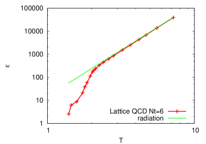
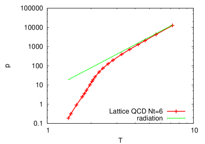
Figure 1: Plot of energy density (left) and pressure (right) versus temperature from Lattice QCD data with $N_{t}=6$. Continuous line is an interpolation through the data. For comparison, we have plotted the expected behavior for radiation.

Lattice QCD is a modern tool which allows one to systematically study the non-perturbative regime of the QCD equation of state. Utilizing supercomputers the QCD equation of state was calculated on the lattice in [12] with two light quarks and a heavier strange quark on a $(N_{t}=6)\times 32^{3}$ size lattice. The quark masses have been chosen to be close to their physical value, i.e. the pion mass is about $220MeV$. For further details we refer the reader to [12], however, we like to remark that the equation of state was calculated at a temporal extent of the lattice $N_{t}=6$ and for $N_{t}=6$ sizable lattice cut-off effects are still present [26].

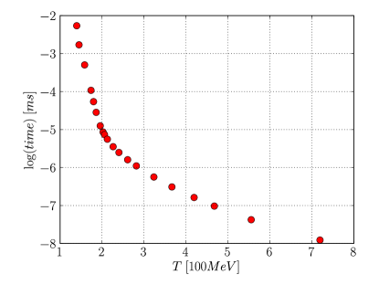
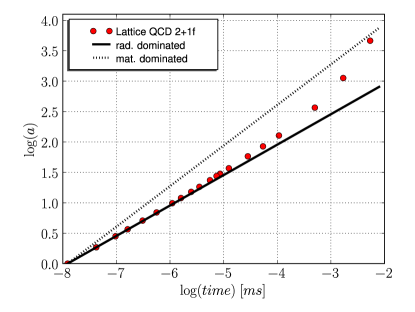
Figure 2: Time versus temperature (left) and time dependence of the scale factor (right) from Lattice QCD data. The behavior of $a(t)$ for radiation (black line) and matter (black dashes) is shown. We set $t_{min}=t(T=719MeV)\equiv(\frac{32\pi G}{3}\varepsilon(T=719MeV))^{-1/2}$ in $ms$ for $a(t_{min})=1.$

The data for energy density $\varepsilon(T)$, pressure $p(T)$ and trace anomaly $\varepsilon-3p$ and entropy $s$ of Ref. [12] are given in Table 1. All the analysis in this section is derived from this data. Besides the strange quark one can also include the effect of the charm quark as well as photons and leptons on the equation of state. These have important cosmological contributions as was shown in [27]. Recent references on lattice QCD at high temperature are [28][29][30].

Table 1: Data from lattice QCD study with $N_{t}=6$ [12]. Temperature in units of $(100MeV)$, Energy density, pressure and trace anomaly in units of $(100MeV)^{4}$, entropy density $s$ in units of $(100MeV)^{3}$.

$T$	$\varepsilon$	$p$	$\varepsilon-3p$	$s$
1.40	2.54	0.189	1.98	1.96
1.45	6.24	0.315	5.30	4.51
1.59	8.88	0.909	6.15	6.17
1.74	21.4	2.45	14.0	13.7
1.80	38.7	3.57	27.9	23.5
1.86	58.7	5.35	42.7	34.4
1.96	113	10.1	82.7	62.9
2.03	170	15.3	124	91.3
2.06	196	18.6	140	104
2.13	238	26.6	158	124
2.27	341	47.3	199	171
2.40	449	74.1	226	218
2.61	635	127	254	292
2.82	859	196	272	375
3.24	1520	398	326	593
3.67	2520	714	377	882
4.19	4350	1300	461	1350
4.68	6800	2070	587	1900
5.56	13800	4300	915	3260
7.19	39300	12600	1480	7220

We plot the energy density and pressure in Figure 1. For comparison, we plot the corresponding curves one would expect for radiation behavior. While for the high temperature regime we see, as expected, radiation like behavior, in the region at and below the critical temperature $T_{c}$ ($\approx 200MeV$) of the deconfinement transition the behavior changes drastically. This change in the behavior will also be relevant for cosmological observables as we will see in the following.

For high temperature between $2.82$ $(100MeV)$ and $7.19$ $(100MeV)$ one can fit the data to a simple equation of state of the form:

$$\begin{array}[]{l}\varepsilon(T)=\alpha_{rad}T^{4}+\dots\\ p(T)=\sigma_{rad}T^{4}+\dots\\ \end{array}$$ (2.1)

We find $\alpha_{rad}=14.9702\pm.009997$ and $\sigma_{rad}=4.99115\pm.004474$ using a least squares fit. The dots indicate terms constant and quadratic in temperature [12].

For lower temperatures the equation of state is very complex and use a numerical procedure to determine $t(T)$, $T(t)$, $\varepsilon(T(t))$ and $a(t)$ using formulas (1.2), (1.3) and (1.4). In Figure 3 we plot $a$ and $\log a$ as a function of $\log t$. The slope of $\frac{1}{2}$ at small times is indicative of expansion due to radiation of the form $a(t)=t^{1/2}$ at high temperatures and early times as discussed in section 1. At late times one see that the scale factor dramatically increases and gives rise to characteristic hockey stick shape pointing northeast. This is reflective of the shape of energy density and pressure plots as a function of temperature which are hockey stick shapes at low temperature pointing southwest. Within this procedure we tried to avoid introducing new systemic uncertainties and keep as close to the lattice data as possible. In Figure 2 we show time vs. temperature (left) and the time dependence of the scale factor (right). We see that in the confinement region, i.e.  for $T$ less than 200 $MeV$ or $\log(t)$ greater than $-5$, the behavior changes. In plot of the right hand side of Figure 2 we also show the behavior of $a(t)$ for radiation and matter. While for times before the phase transition the lattice data matches with the radiation behavior very well, for times corresponding to temperatures above $T_{c}$ the behavior of the lattice data changes towards matter dominated behavior. We remark that lattice studies show that the QCD phase transition at its physical values is actually a cross-over phase transition. Therefore, the change in the scale factor we observe is rather moderate and is in contrast to a scenario one would expect, e.g., from a first order phase transition.

Besides lattice QCD there are other approaches to the low temperature equation of state. In the following sections we compare the prediction of some of these approaches for $\varepsilon(T)$, $p(T)$ and the scale factor $a(t)$ to the results from lattice QCD. In particular we shall discuss how well various models can describe the characteristic shape of the $\log a$ versus $t$ curves coming from lattice QCD.

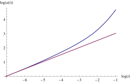
Figure 3: Scale factor and log of scale factor as function of log time from lattice equation of state. Lower curve is the result from radiation. A different fitting procedure using interpolation as opposed to Figure 2. This lead to a larger value for the scale factor. In this figure we set $\log t_{min}=\log t(T=719MeV)=-7.045967106$

3 Hadronic resonance gas model

In the framework the Hadronic Resonance Gas model (HRG), QCD in the confinement phase is treated as an non-interacting gas of fermions and bosons [21, 22, 23, 24]. The fermions and bosons in this model are the hadronic resonances of QCD, namely mesons and baryons. The idea of the HRG model is to implicitly account for the strong interaction in the confinement phase by looking at the hadronic resonances only since these are basically the relevant degrees of freedom in that phase. The HRG model is expected to give a good description of thermodynamic quantities in the transition region from high to low temperature [31].

The partition function of the HRG model is given by a sum of one particle partition functions,

$$\log Z(T,V)=\sum_{i}\log Z^{1}_{i}(T,V)=\sum_{i}\frac{Vg_{i}}{2\pi^{2}}\int_{0}^{\infty}dp\,p^{2}\eta_{i}\log(1+\eta_{i}\mathrm{e}^{-\beta E_{i}}).$$ (3.1)

The HRG model includes hadronic masses $m_{i}$ and degeneracies $d_{i}$ in a low energy statistical model. The equation of state is given by:

$$\begin{array}[]{l}\varepsilon(T)=\sum\nolimits_{m_{i}}{\frac{{d_{i}}}{{2\pi^{2}}}}\sum\limits_{k=1}^{\infty}{(-\eta_{i})^{k+1}m_{i}^{4}}((\frac{T}{{km_{i}}})K_{1}(km_{i}/T)+3(\frac{T}{{km_{i}}})^{2}K_{2}(km_{i}/T)),\\ p(T)=\frac{1}{3}\sum\nolimits_{m_{i}}{\frac{{d_{i}}}{{2\pi^{2}}}}\sum\limits_{k=1}^{\infty}{(-\eta_{i})^{k+1}m_{i}^{4}}3(\frac{T}{{km_{i}}})^{2}K_{2}(km_{i}/T).\end{array}$$

Here $\eta_{i}=-1$ for bosons and $\eta_{i}=1$ for fermions and $K_{1}(z)$ and $K_{2}(z)$ are modified Bessel functions. For practical reasons we performed the sum over $m_{i}$ up to $m_{max}=2.5GeV$.

We plot the energy density and pressure as a function of temperature in Figure 4. Over the temperature range of the the lattice QCD data the HRG model gives values of the energy density and pressure that exceed the lattice QCD data as shown in Figure 5 [12]. If one derives the scale factor between 1.39 and 1.95 in units of 100 MeV one sees a power expansion with coefficient .605 which is less than the matter dominated result of $2/3$ as shown in Figure 6. This is reasonable as this region of temperature is intermediate between the matter dominated phase with expansion exponent $2/3$ and radiation dominated phase with expansion coefficient $1/2$. The HRG model equation of state is expected to be valid at low temperatures with matter dominated expansion. As the temperature is increased the value of the expansion exponent drops as one enters the regime best described by high temperature lattice QCD. Ultimately in the full QCD theory the expansion exponent drops as one reaches deconfinement where the theory is described by a quark-gluon plasma.

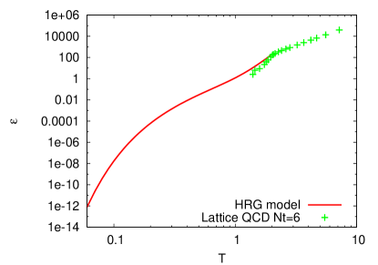
Figure 4: Energy density and pressure from the HRG equation of state. The crosses are lattice QCD data with $N_{t}=6$

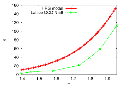
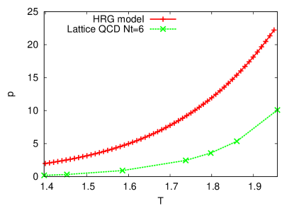
Figure 5: Energy density and pressure from the HRG equation of state over the range of temperatures covered by the lattice QCD calculation. The crosses are lattice QCD data with $N_{t}=6$.

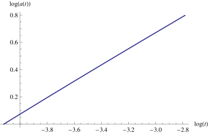
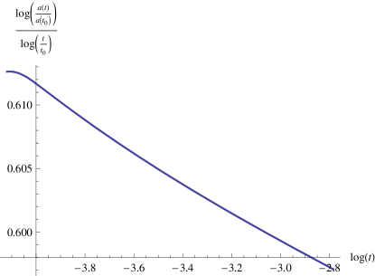
Figure 6: HRG model $\log a(t)$ as a function of $\log t$. The time range corresponds to temperatures from 1.39 to 1.95 in units of 100 MeV. The slope is approximately .605 which is approaching the matter dominated value of .666. Here $t_{0}$ is .0162553.

4 Hagedorn model

This model is similar to the HRG model except the degeneracy factors take a string type dependence on mass [10, 11]. The energy density and pressure are given by:

$$\begin{array}[]{l}\varepsilon(T)=\int{dm\rho(m)\int{\frac{{d^{3}k}}{{(2\pi)^{3}}}}}\frac{1}{{e^{E(k,m)/T}+1}}E(k,m),\\ p(T)=\frac{1}{3}\int{dm\rho(m)\int{\frac{{d^{3}k}}{{(2\pi)^{3}}}}}\frac{1}{{e^{E(k,m)/T}+1}}\frac{{k^{2}}}{{E(k,m)}}\end{array}$$

where $E(k,m)=\sqrt{k^{2}+m^{2}}$. The degeneracy function $\rho(m)$ is given by:

$$\rho(m)=cm^{-\gamma}\exp(\frac{m}{T_{H}}).$$

for large mass $m$ and some exponent $\gamma$. These formulas have simple generalizations to nonzero chemical potential, although we restrict ourselves to zero chemical potential in this paper. The integrals over $m$ and momentum can be done using the methods of Carlitz [32]. For $\gamma=5/2$ one has the equation of state:

$$\begin{array}[]{l}p(T)=\alpha_{0}(\frac{T}{{T_{H}}})^{5/2}\Gamma(\frac{{m_{0}(T_{H}-T)}}{{T_{H}T}},0),\\ \varepsilon(T)=\frac{\alpha_{0}}{{T_{H}}}T^{2}\partial_{T}((\frac{T}{{T_{H}}})^{3/2}\Gamma(\frac{{m_{0}(T_{H}-T)}}{{T_{H}T}},0))\end{array}$$

where $\Gamma(x,\frac{5}{2}-\gamma)=\int^{\infty}_{x}e^{-y}y^{3/2-\gamma}dy$. For $\gamma=5/2$ this is the exponential integral $E_{1}(x)=\int^{\infty}_{x}e^{-y}y^{-1}dy$.

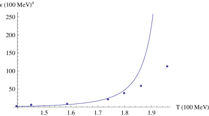
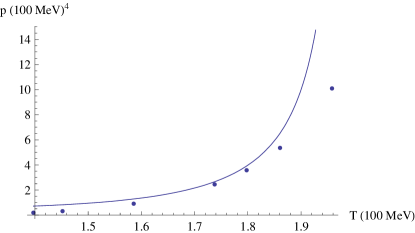
Figure 7: Energy density and pressure from the Hagedorn equation of state over the range of temperatures covered by the lattice QCD calculation. The dots are lattice QCD data with $N_{t}=6$.

Pressure and energy density are are plotted in Figure 7 for $T_{H}=200MeV$, $\alpha_{0}=1.96665(100MeV)^{4}$ and $m_{0}=6.10776(100MeV)$ alongside the lattice data. The energy density displays a limiting temperature so we study the equation of state of the Hagedorn model as a model of low energy QCD below $T_{H}$ only. The approach of using a string-like model with a limiting temperature to describe the strong interactions has a long history. A modern perspective on the approach is given in [33, 34, 35]. In $TeV$ scale gravity a $TeV$ Hagedorn temperature is possible if the string scale turns out to be at a few $TeV$[36]. A Hagedorn type cosmology in the early Universe is proposed as alternative to inflation in with the Hagedorn temperature at two orders of magnitude below the Planck scale [37]. A nice discussion at the popular level of the concept of limiting temperature or absolute hot is given in [38].

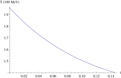
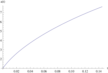
Figure 8: Temperature and scale factor as a function of time from the Hagedorn equation of state.

Given the equation of state we can use the methods of the previous section to determine the temperature a function of time as well as the scale factor $a(t)$ which are shown in Figure 8. Note from Figure 8 the temperature is less than $T_{H}$ for all times in the Hagedorn model of cosmology. This shows the limiting temperature nature of the Hagedorn cosmology. Another feature of the Hagedorn cosmology is that $a(t)$ in Figure 8 is more complex than a power law as was shown in [11]. The Hagedorn cosmology is not considered a leading cosmological theory at this time mainly because temperatures higher than $T_{H}$ can be observed in the early Universe. However for theories where the Hagedorn temperature is at the TeV scale or at the Planck length the Hagedorn cosmology is still of interest.

5 AdS/CFT model of low energy QCD

Determining the time dependence of the scale factor $a(t)$ is not one of the strong points of the AdS/CFT correspondence. This is because the only gravity in the correspondence is induced in the AdS five dimensional space and there is no dynamical gravity on the CFT side which one wants to identify with a QCD-like theory. Thus questions like what happens when a glue-ball falls into a black hole or even how a proton is attracted to the earth can’t be straightforwardly addressed within $AdS_{5}/CFT_{4}$. One has to use another approach with gravity and matter on the same side of the correspondence. Nevertheless, recently Gubser and Nellore [13] have determined a low energy equation of state for a QCD-like theory using $AdS^{5}/CFT_{4}$ and these can be used to calculate the back reaction on Einstein’s equation to leading order.

We first consider $AdS$ gravity without dilaton or with dilaton equal to zero, where the entropy and mass can be determined analytically. We then consider refinements from including the dilaton and a numerical treatment similar to [13] to determine the entropy and mass. Then using the conjectured duality between the AdS black hole and CFT theories we obtain the entropy and energy density of the dual gauge theory and it’s equation of state. Finally one can use this entropy and energy density to determine the expansion factor $a(t)$ associated with the dual gauge theory by using Einstein’s equations on the the dual gauge side of the correspondence.

5.1 $AdS^{5}$ gravity without the dilaton

We work within the ansatz for the five dimensional metric given by:

$$ds^{2}=c^{2}(r)(-dt^{2})+b^{2}(r)dr^{2}+\tilde{a}^{2}(r)d\Omega_{3}^{2}.$$

We use a tilde to differentiate the dual variable $\tilde{a}$ from the scale factor $a$ that occurs in the physical four dimensional metric. We denote the metric for the unit three sphere by $d\Omega_{3}^{2}$.

The equations of motion within this ansatz follow from the Lagrangian:

$$L=\left(6\frac{{\tilde{a}^{\prime 2}}}{{\tilde{a}^{2}b}}+6\frac{{\tilde{a}^{\prime}}}{{\tilde{a}}}\frac{{c^{\prime}}}{{bc}}+6\frac{b}{{\tilde{a}^{2}}}+\tilde{\lambda}b-\frac{{\phi^{\prime 2}}}{{2b}}-V(\phi)b\right)\tilde{a}^{3}c$$

which comes from the Einstein-Hilbert Lagrangian:

$$\sqrt{-g}(R+\tilde{\lambda}-\frac{1}{2}(\partial\phi)^{2}-V(\phi)).$$

Where $-\tilde{\lambda}$ denotes the cosmological constant of the dual $AdS$ space and $V(\phi)$ is a potential of a scalar field $\phi$. We impose the gauge condition:

$$cb=1.$$

In this gauge the equations of motion become:

$$\begin{array}[]{l}12\alpha^{\prime\prime}+18\alpha^{\prime 2}+24\alpha^{\prime}\beta^{\prime}+6\beta^{\prime\prime}+12\beta^{\prime 2}-6e^{2\alpha-2\beta}-3\tilde{\lambda}e^{-2\beta}+\frac{3{\phi^{\prime 2}}}{2}+3V(\phi)e^{-2\beta}=0\\ 6\alpha^{\prime\prime}+6\alpha^{\prime 2}+\phi^{\prime 2}=0\\ \phi^{\prime\prime}+3\phi^{\prime}\alpha^{\prime}+2\phi^{\prime}\beta^{\prime}-\frac{{dV(\phi)}}{{d\phi}}e^{-2\beta}=0\\ \end{array}$$

where we have defined $\alpha=\log{\tilde{a}}$ and $\beta=\log c$.

The equations have the solution in vacuum $\phi=0$ and $V(\phi)=0$ given by:

$$\begin{array}[]{l}\tilde{a}=r\\ b=(1-\frac{\mu}{r^{2}}+\frac{\tilde{\lambda}}{12}r^{2})^{-1/2}\\ c=(1-\frac{\mu}{r^{2}}+\frac{\tilde{\lambda}}{12}r^{2})^{1/2}\\ \end{array}$$

In this solution $\mu$ is a constant parameter which turns out to be be proportional to the mass of the black hole. The horizon is determined by the largest solution to $c(r_{+})=0$ and is given by:

$$r_{+}=\mu^{1/2}\frac{\sqrt{2}}{\sqrt{{{1+\frac{{\sqrt{3+\mu\tilde{\lambda}}}}{\sqrt{3}}}}}}.$$

The entropy can be computed from the formula:

$$S=\frac{{\omega_{3}}}{4}\tilde{a}^{3}\tilde{m}_{P}^{3}|_{r=r_{+}}.$$

where $\omega_{3}=2\pi^{2}$ is the volume of a unit three sphere and $\tilde{m}_{P}$ is the five dimensional Planck mass in the dual space. The temperature of the black hole solution is determined from:

$$T=\frac{1}{{4\pi}}\frac{{\tilde{a}^{2}}}{{cb}}(\frac{c^{2}}{\tilde{a}^{2}})^{\prime}|_{r=r_{+}}.$$

One can define a mass formula similar to that of Poisson and Israel [39] and Fischler, Morgan and Polchinski [40] for spherically symmetric gravity. It is given by:

$$M=\frac{3\omega_{3}}{16\pi}\tilde{m}_{P}^{3}\tilde{a}^{2}(1-\frac{{\tilde{a}^{\prime 2}}}{{b^{2}}}+\frac{{\tilde{\lambda}}}{{12}}\tilde{a}^{2})|_{r=\infty}.$$

Applying these formula to the above solution the entropy is given by:

$$S=\frac{{\omega_{3}}}{4}\mu^{3/2}\tilde{m}_{P}^{3}\left({\frac{2}{{1+\frac{{\sqrt{3+\mu\tilde{\lambda}}}}{{\sqrt{3}}}}}}\right)^{3/2}$$

and temperature is

$$T=\frac{1}{2{\pi\mu^{1/2}}}\sqrt{\frac{{1+\frac{{\sqrt{3+\mu\tilde{\lambda}}}}{{\sqrt{3}}}}}{2}}\frac{{\sqrt{3+\mu\tilde{\lambda}}}}{{\sqrt{3}}}.$$

The mass formula simply reduces to:

$$M=\frac{3\omega_{3}}{16\pi}\mu\tilde{m}_{P}^{3}.$$

This solution satisfies:

$$T=(\frac{\partial S}{\partial M})^{-1}$$

in analogy with classical thermodynamics [41, 42, 43]. Expanding the expressions for entropy and mass as a function of temperature for large mass one finds:

$$S\tilde{m}_{P}^{3}=\frac{1}{2}\pi^{5}(\frac{12}{\tilde{\lambda}})^{3}\tilde{m}_{P}^{6}T^{3}+\dots$$

and

$$M\tilde{m}_{P}^{3}=\frac{3}{8}\pi^{5}(\frac{12}{\tilde{\lambda}})^{3}\tilde{m}_{P}^{6}T^{4}+\dots$$

Matching these expressions to the lattice QCD data for entropy and energy density at high temperatures from formula (2.1) one finds that

$$\tilde{\lambda}\approx 23.661\tilde{m}_{P}^{2}.$$

The entropy and mass of the $AdS^{5}$ black hole solution without dilaton are plotted in Figure 9.

Table 2: Quantities used to compare $AdS^{5}$ gravity and finite temperature QCD cosmology.

Quantity	$AdS^{5}$ gravity	QCD cosmology
entropy	$S\tilde{m}_{P}^{3}$	$s$
energy density	$M\tilde{m}_{P}^{3}$	$\varepsilon$
temperature	$T_{Hawking}$	$T$
fields	$\tilde{a}(r),b(r),c(r),\phi(r)$	$a(t)$
fundamental constants	$\tilde{m}_{P}$, $\tilde{\lambda}$	$M_{P}$, $\lambda$

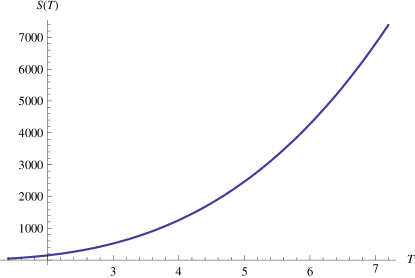
Figure 9: Entropy and mass (energy density) of the $AdS^{5}$ black hole as function of temperature without the dilaton.

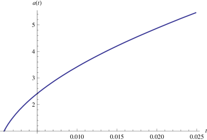
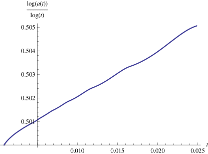
Figure 10: Time dependence of radius $a(t)$ determined from dual $AdS^{5}$ black hole solution without the dilaton.

Rewriting the equation (1.2) that determines the time dependence of the temperature in terms of entropy and energy density we have:

$$\frac{{dT}}{{dt}}=-3(Ts)\sqrt{\frac{{\varepsilon(T)}}{3M_{P}^{2}}}(\frac{{d\varepsilon(T)}}{{dT}})^{-1}.$$ (5.1)

Then using the correspondence from Table 2 one can determine the radius of the 4d universe $a(t)$ from (5.1). This is plotted in Figure 10. One can see from the plot on right hand side of Figure 10 that over the temperature range covered by the lattice QCD data one never leaves the radiation regime and the scale factor is well approximated by $a(t)=t^{1/2}$.

In this AdS approach it is is important not to confuse the scale factor $a(t)$ with the dual radius $\tilde{a}(r)$. One uses the black hole solution including $\tilde{a}(r)$ to determine the entropy, temperature and energy density and then uses (5.1) to determine the scale factor $a(t)$ through the correspondence in Table 2.

5.2 $AdS^{5}$ gravity with nonzero dilaton

Because the vacuum solution to $AdS^{5}$ gravity does not match with the lattice QCD data at low temperature and stays in the radiation regime over the temperature range of lattice QCD, one looks for non vacuum solutions that can mimic the lattice QCD equation of state. In [13] the potential

$$V(\phi)=\tilde{\lambda}(1-\cosh(2.057\phi)+\tilde{\lambda}\frac{0.606}{12}\phi^{2}$$ (5.2)

was used to describe a $AdS^{5}$ black hole with nonzero dilaton field. For nonzero $\phi$ and $V(\phi)$ one can solve the equations of motion numerically. In [13] it was shown that the speed of sound associated with the potential (5.2) closely approximates the speed of sound from lattice QCD.

For nonzero dilaton it is convenient to replace the coordinate $r$ by $1/z$. Then the asymptotic region $r=\infty$ corresponds to $z=0$. In the coordinate $z$, the five dimensional metric ansatz is taken to be:

$$ds^{2}=c^{2}(z)(-dt^{2})+b^{2}(z)dz^{2}+\tilde{a}^{2}(z)d\Omega_{3}^{2}.$$

It is convenient to choose the gauge:

$$cb=\tilde{a}^{2}.$$

In this gauge the equations of motion become:

$$\begin{array}[]{l}12\alpha^{\prime\prime}+6\alpha^{\prime 2}+24\alpha^{\prime}\beta^{\prime}+6\beta^{\prime\prime}+12\beta^{\prime 2}-18e^{2\alpha-2\beta}-5\tilde{\lambda}e^{4\alpha-2\beta}+\frac{{\phi^{\prime 2}}}{2}+5V(\phi)e^{4\alpha-2\beta}=0\\ 6\alpha^{\prime\prime}-6\alpha^{\prime 2}+\phi^{\prime 2}=0\\ \phi^{\prime\prime}+\phi^{\prime}\alpha^{\prime}+2\phi^{\prime}\beta^{\prime}-\frac{{dV(\phi)}}{{d\phi}}e^{4\alpha-2\beta}=0\\ \end{array}$$ (5.3)

where the prime refers to the derivative with respect to $z$ and as before where we have defined $\alpha=\log{\tilde{a}}$ and $\beta=\log c$.

We found that the asymptotic form of the dilaton at small $z$ had an important effect on the values of the entropy and mass of the black hole thus one needs to carefully study the effects of various dilaton boundary conditions to mimic the lattice QCD equation of state. In the asymptotic regime near for small $z$ we seek a black hole solution to to the equations of motion with a small asymptotic value for the dilaton field $\phi(z)$.

For small $z$ we set:

$$\begin{array}[]{l}\tilde{a}=\frac{1}{z}e^{-\sigma\frac{1}{36}z^{2}}\\ b=\frac{1}{z^{2}}e^{-\sigma\frac{1}{36}z^{2}}(1-\mu z^{2}+\frac{\tilde{\lambda}}{12z^{2}})^{-1/2}\\ c=e^{-\sigma\frac{1}{36}z^{2}}(1-\mu z^{2}+\frac{\tilde{\lambda}}{12z^{2}})^{1/2}\\ \end{array}$$

where $\sigma$ is a deformation parameter. In terms of $\alpha$ and $\beta$ this becomes:

$$\begin{array}[]{l}\alpha=-\log z-\sigma\frac{1}{36}z^{2}\\ \beta=\frac{1}{2}\log(1-\mu z^{2}+\frac{\tilde{\lambda}}{12z^{2}})-\sigma\frac{1}{36}z^{2}\\ \end{array}$$

One can then use the second equation in (5.3) to solve for the asymptotic form of the dilaton by integrating:

$$\phi^{\prime}=\sqrt{-6\alpha^{\prime\prime}+6\alpha^{\prime 2}}$$

as in [44]. This leads to the asymptotic form of the dilaton:

$$\phi=\frac{1}{6\sqrt{6}}\sqrt{\sigma}z\sqrt{54+z^{2}\sigma}+54\frac{1}{6\sqrt{6}}\sinh^{-1}(\frac{z\sqrt{\sigma}}{3\sqrt{6}}).$$

Expanding this expression for small $z$ we find:

$$\phi=\sqrt{\sigma}z+\frac{1}{324}\sigma^{3/2}z^{3}-\frac{1}{116640}\sigma^{5/2}z^{5}+\frac{1}{17635968}\sigma^{7/2}z^{7}+\dots$$

One can use this expression to define a boundary condition on the dilaton field for small $z$. Then one can numerically solve for the black hole solution with potential (5.2) and a given deformation parameter $\sigma$. As $\sigma$ goes to zero one has the vacuum black hole solution discussed in the previous subsection.

For $\sigma=.01$ the entropy, mass (energy density), and temperature are all modified by the dilaton. In Figure 11 we plot the entropy and mass as a function of temperature for $\sigma=.01$. One can then use equation (5.1) to calculate the time dependence of the physical radius $a(t)$. This is shown in Figure 12. The inclusion of the dilaton creates nontrivial deviation from the radiation type expansion at late times and low temperatures. In particular, we observe in Figure 12 the upward bending hockey stick behavior that is qualitatively similar to that of lattice QCD.

Without the dilaton the scale factor $a(t)$ can be described by the radiation expression $t^{1/2}$ over the temperature range covered by the lattice QCD calculation. With the dilaton it is possible to describe a late time behavior similar to lattice QCD.

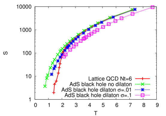
Figure 11: Comparison of entropy and mass (energy density) between Lattice QCD with $Nt=6$ and $AdS$ black hole solutions with and without the dilaton.

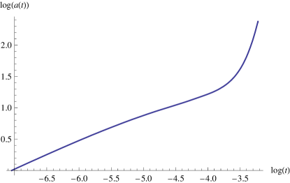
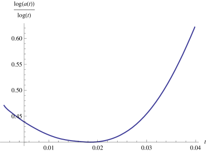
Figure 12: Scale factor as a function of log time from $AdS$ black hole equation of state with dilaton.

6 Conclusion

We have computed the time dependence of the scale factor from the lattice QCD equation of state with $N_{t}=6$. We find that the scale factor is described by a radiation dominated universe $t^{1/2}$ at early times with a complicated time dependence at late times which seems to be closer to a matter dominated universe. We compared our results from lattice QCD with other approaches to the low temperature equation of state including the hadronic resonance gas model, the Hagedorn model and the AdS/CFT equation of state.

We found that on a log log plot the scale factor displayed an upward pointing hockey stick behavior for the lattice QCD data. For the hadronic resonance gas model over the temperature range of lattice QCD data, the HRG model lies above the lattice QCD data [12]. The slope of the log log plot for the scale factor is between the radiation value .5 and the matter dominated value .666 for the HRG model in this regime. The Hagedorn model leads to a limiting temperature as a function of time and works better a low temperature and late times. The equations are simpler than the HRG model because less experimental input is required but lead to a diverging energy density at the Hagedorn temperature unlike the lattice QCD data. The Hagedorn cosmological model is still of interest for theories where the limiting temperature is at the TeV scale or the Planck scale. For the AdS/QCD model we found that without the dilaton the entropy and energy density led to a $t^{1/2}$ expansion over the temperature range of lattice QCD. We introduced a parameter $\sigma$ that determined the boundary condition at infinity for the dilaton. Turning the dilaton on and tuning the parameter $\sigma$ allowed us to derive a time dependence for the scale factor that was qualitatively similar to that of lattice QCD through the AdS/QCD correspondence.

With future improvements in lattice QCD calculations and deeper understanding of the role of AdS/QCD it will be interesting to revisit the subject of QCD cosmology by adding the effects of bulk viscosity, chemical potentials and interaction with leptons. Eventually one would like to make contact with astrophysical measurements of the early Universe as envisioned in early references such as [1].

References

- [1] E. Witten, “Cosmic Separation Of Phases,” Phys. Rev. D 30, 272 (1984).
- [2] D. J. Schwarz, “The first second of the universe,” Annalen Phys. 12, 220 (2003) [arXiv:astro-ph/0303574].
- [3] L. M. Müller, Master’s thesis, “The quark-hadron phase transition in the early Universe”, (2001).
- [4] N. Borghini, W. N. Cottingham and R. Vinh Mau, “Possible cosmological implications of the quark-hadron phase transition,” J. Phys. G 26, 771 (2000) [arXiv:hep-ph/0001284].
- [5] J. I. Kapusta, “Quark-gluon plasma in the early universe,” arXiv:astro-ph/0101516.
- [6] D. Chandra and A. Goyal, “Dynamical evolution of the universe in the quark-hadron phase transition and possible nugget formation,” Phys. Rev. D 62, 063505 (2000) [arXiv:hep-ph/9903466].
- [7] A. A. Coley and T. Trappenberg, “The Quark - hadron phase transition, QCD lattice calculations and inhomogeneous big bang nucleosynthesis,” Phys. Rev. D 50, 4881 (1994) [arXiv:astro-ph/9307031].
- [8] H. Suganuma, H. Ichie, H. Monden, S. Sasaki, M. Orito, T. Yamamoto and T. Kajino, “QCD phase transition at high temperature in cosmology,” arXiv:hep-ph/9608333.
- [9] K. A. Olive, “The Quark - hadron transition in cosmology and astrophysics,” Science 251, 1194 (1991).
- [10] R. Hagedorn, “Statistical thermodynamics of strong interactions at high-energies,” Nuovo Cim. Suppl. 3, 147 (1965).
- [11] K. Huang and S. Weinberg, “Ultimate temperature and the early universe,” Phys. Rev. Lett. 25, 895 (1970).
- [12] M. Cheng et al., “The QCD Equation of State with almost Physical Quark Masses,” Phys. Rev. D 77, 014511 (2008) [arXiv:0710.0354 [hep-lat]].
- [13] S. S. Gubser and A. Nellore, “Mimicking the QCD equation of state with a dual black hole,” arXiv:0804.0434 [hep-th].
- [14] S. S. Gubser, A. Nellore, S. S. Pufu and F. D. Rocha, “Thermodynamics and bulk viscosity of approximate black hole duals to finite temperature quantum chromodynamics,” arXiv:0804.1950 [hep-th].
- [15] S. S. Gubser, S. S. Pufu and F. D. Rocha, “Bulk viscosity of strongly coupled plasmas with holographic duals,” arXiv:0806.0407 [hep-th].
- [16] B. Freedman and L. D. McLerran, “Quark Star Phenomenology,” Phys. Rev. D 17, 1109 (1978).
- [17] S. Chakrabarty, “Equation of state of strange quark matter and strange star,” Phys. Rev. D 43, 627 (1991).
- [18] W. M. Yao et al. [Particle Data Group], “Review of particle physics,” J. Phys. G 33, 1 (2006).
- [19] M. Luzum and P. Romatschke, “Conformal Relativistic Viscous Hydrodynamics: Applications to RHIC,” arXiv:0804.4015 [nucl-th].
- [20] D. Kharzeev and K. Tuchin, “Bulk viscosity of QCD matter near the critical temperature,” arXiv:0705.4280 [hep-ph].
- [21] F. Karsch, K. Redlich and A. Tawfik, “Hadron resonance mass spectrum and lattice QCD thermodynamics,” Eur. Phys. J. C 29, 549 (2003) [arXiv:hep-ph/0303108].
- [22] F. Karsch, K. Redlich and A. Tawfik, “Thermodynamics at non-zero baryon number density: A comparison of lattice and hadron resonance gas model calculations,” Phys. Lett. B 571, 67 (2003) [arXiv:hep-ph/0306208].
- [23] K. Sakthi Murugesan, G. Janhavi and P. R. Subramanian, “Can the phase transition from quark - gluon plasma to hadron resonance gas affect primordial nucleosynthesis?,” Phys. Rev. D 41, 2384 (1990).
- [24] A. Tawfik, “The QCD phase diagram: A comparison of lattice and hadron resonance gas model calculations,” Phys. Rev. D 71, 054502 (2005) [arXiv:hep-ph/0412336].
- [25] M. Shifman and M. Unsal, “QCD-like Theories on : a Smooth Journey from Small to Large with Double-Trace Deformations,” arXiv:0802.1232 [hep-th].
- [26] R. Gupta, “The EOS from simulations on BlueGene L Supercomputer at LLNL and NYBlue,“ PoS LAT2008 170 (2008)
- [27] M. Laine and Y. Schroder, “Quark mass thresholds in QCD thermodynamics,” Phys. Rev. D 73, 085009 (2006) [arXiv:hep-ph/0603048].
- [28] M. Cheng [RBC-Bielefeld Collaboration], “Charm Quarks and the QCD Equation of State,” PoS LAT2007, 173 (2007) [arXiv:0710.4357 [hep-lat]].
- [29] G. Endrodi, Z. Fodor, S. D. Katz and K. K. Szabo, “The equation of state at high temperatures from lattice QCD,” PoS LAT2007, 228 (2007) [arXiv:0710.4197 [hep-lat]].
- [30] D. E. Miller, “Lattice QCD calculation for the physical equation of state,” Phys. Rept. 443, 55 (2007) [arXiv:hep-ph/0608234].
- [31] P. Braun-Munzinger, K. Redlich and J. Stachel, “Particle production in heavy ion collisions,” arXiv:nucl-th/0304013; A. Andronic, P. Braun-Munzinger and J. Stachel, “Hadron production in central nucleus nucleus collisions at chemical freeze-out,” Nucl. Phys. A 772, 167 (2006) [arXiv:nucl-th/0511071].
- [32] R. D. Carlitz, “Hadronic matter at high density,” Phys. Rev. D 5, 3231 (1972).
- [33] P. Castorina, D. Kharzeev and H. Satz, “Thermal Hadronization and Hawking-Unruh Radiation in QCD,” Eur. Phys. J. C 52, 187 (2007) [arXiv:0704.1426 [hep-ph]].
- [34] T. Harmark and M. Orselli, “Matching the Hagedorn temperature in AdS/CFT,” Phys. Rev. D 74, 126009 (2006) [arXiv:hep-th/0608115].
- [35] S. Kalyana Rama and B. Sathiapalan, “The Hagedorn transition, deconfinement and the AdS/CFT correspondence,” Mod. Phys. Lett. A 13, 3137 (1998) [arXiv:hep-th/9810069].
- [36] I. Antoniadis and B. Pioline, “Large dimensions and string physics at a TeV,” arXiv:hep-ph/9906480.
- [37] A. Nayeri, R. H. Brandenberger and C. Vafa, “Producing a scale-invariant spectrum of perturbations in a Hagedorn phase of string cosmology,” Phys. Rev. Lett. 97, 021302 (2006) [arXiv:hep-th/0511140].
-
[38]
P. Tyson, “Absolute Hot: Is there an opposite to absolute zero?”
http://www.pbs.org/wgbh/nova/zero/hot.html - [39] E. Poisson and W. Israel, “Internal structure of black holes,” Phys. Rev. D 41, 1796 (1990).
- [40] W. Fischler, D. Morgan and J. Polchinski, “Quantization of false vacuum bubbles:A Hamiltonian treatment of gravitational tunneling,” Phys. Rev. D 42, 4042 (1990).
- [41] N. Pidokrajt, “Black hole thermodynamics”, master’s thesis (2003).
- [42] J. Louko, J. Z. Simon and S. N. Winters-Hilt, “Hamiltonian thermodynamics of a Lovelock black hole,” Phys. Rev. D 55, 3525 (1997) [arXiv:gr-qc/9610071].
- [43] H. Quevedo and A. Sanchez, “Geometrothermodynamics of asymptotically de Sitter black holes,” arXiv:0805.3003 [hep-th].
- [44] W. de Paula, T. Frederico, H. Forkel and M. Beyer, “Dynamical AdS/QCD with area-law confinement and linear Regge trajectories,” arXiv:0806.3830 [hep-ph].