Quantum search by parallel eigenvalue adiabatic passage

Abstract

We propose a strategy to achieve the Grover search algorithm by adiabatic passage in a very efficient way. An adiabatic process can be characterized by the instantaneous eigenvalues of the pertaining Hamiltonian, some of which form a gap. The key to the efficiency is based on the use of parallel eigenvalues. This allows us to obtain non-adiabatic losses which are exponentially small, independently of the number of items in the database in which the search is performed.

I Introduction

Quantum computation by adiabatic evolution has been proposed as a general method of solving search problems, mainly to exploit its robustness towards unitary control errors and decoherence adiabatic1 ; adiabatic2 . In contrast to the standard paradigm of quantum computation nielsen , which is implemented through gates embedded in a quantum circuit, continuous-time algorithms farhi , and in particular adiabatic ones adiabatic1 ; adiabatic2 ; RC proceed through the controlled evolution of some Hamiltonians designed to solve the specified problem. The adiabatic Grover algorithm, for instance, involves a time-dependent Hamiltonian which smoothly drives the system, in a time exhibiting a quadratic speedup, from one of its eigenstates $|w\rangle$ that is easily prepared to a connected eigenstate that coincides with the marked entry $|m\rangle$ of the database. This can be achieved with the two-parameter Hamiltonian

$$H=a(t)H_{\text{i}}+b(t)H_{\text{f}},$$ (1)

where $H_{\text{i}}=|w\rangle\langle w|$ and $H_{\text{f}}=|m\rangle\langle m|$ are simply projectors on the appropriate states while $a$ and $b$ are time-dependent parameters which vanish at the final and initial times, respectively, to ensure that the prepared and target states are eigenstates. The eigenstates of $H$ form in general an avoided crossing as a function of time. The search is achieved when the dynamics follows adiabatically the instantaneous eigenstate connected initially to the prepared state $|w\rangle$ and finally to the marked state $|m\rangle$. The way the parameters $a$ and $b$ vary around the avoided crossing is key to making the search exhibit or not a quadratic speedup. It has been shown that achieving a quadratic speedup requires a non-linear dynamics of the parameters: The dynamics has to slow down when approaching the smallest gap of the avoided crossing and has to accelerate afterwards RC . This strategy will be referred to as local strategy. In this paper we apply the strategy of optimal adiabatic passage developed in Refs. Leveline ; GJ for two-level models of the form (with real couplings)

$$H=\left[\begin{array}[]{cc}\Delta(t)&\Omega(t)\\ \Omega(t)&-\Delta(t)\end{array}\right].$$ (2)

It has been shown that, for a given smooth pulsed-shape coupling of the form $\Omega(t)=\Omega_{0}\Lambda(t)$ (with $\Lambda(\pm\infty)=0$) and for the parametrization $\Delta(t)/\Delta_{0}+\Omega(t)/\Omega_{0}=1$, the population transfer is the most efficient, in the adiabatic regime, when the instantaneous eigenvalues are parallel. This corresponds to $\Delta_{0}=\Omega_{0}$, i.e. to level lines (corresponding to circles of equation $\Omega(t)^{2}+\Delta(t)^{2}=\Delta_{0}^{2}$) in the diagram of the difference of the eigenvalue surfaces as a function of the two parameters $\Omega(t)$ and $\Delta(t)$. We show that this strategy, referred to as parallel strategy, applied to the problem of quantum search using the two-parameter Hamiltonian (1) leads to a Grover type search, i.e. scaling with time as $\sqrt{N}$. It is moreover more efficient than the local strategy proposed in Ref. RC since it allows one to increase the success rate to hit the searched state. The paper is organized as follows. In Sec. II, we describe the model and the strategies to achieve the quantum search. In particular, the local and parallel strategies are presented. Section III is devoted to the definition of a cost and the calculation of the non-adiabatic losses which are used to define the optimality and to compare the local and parallel strategies. The comparison is illustrated numerically in Sec. IV while the conclusions are given in Sec. V.

II Model and strategies

The marked state $|m\rangle$ is one of the computational basis states $|1\rangle,\cdots,|N\rangle$. The two-parameter Hamiltonian (3) can be rewritten in an orthogonal basis which features the marked state $|m\rangle$ and the uniform superposition of unmarked states, $|u\rangle=\sum_{i\neq m}\frac{1}{\sqrt{N-1}}|i\rangle$,

$$H = \left(\frac{a+b}{2}-\Delta\right)|m\rangle\langle m|+\left(\frac{a+b}{2}+\Delta\right)|u\rangle\langle u|$$ (3)

$$+ \Omega\left(|u\rangle\langle m|+|m\rangle\langle u|\right),$$

with $\Omega=a\sqrt{N-1}/N$ and $\Delta=(a-b)/2-a/N$. Its eigenvalues are

$$\lambda_{\pm}=\frac{a+b}{2}\pm\frac{1}{2}\sqrt{a^{2}+b^{2}-2ab\left(1-\frac{2}{N}\right)},$$ (4)

and the pertaining eigenvectors read

$$|+\rangle =\cos\theta|u\rangle+\sin\theta|m\rangle,\quad\tan 2\theta=\frac{\Omega}{\Delta},\quad\theta\in[0,\pi/2[$$

$$|-\rangle =\sin\theta|u\rangle-\cos\theta|m\rangle.$$ (5)

In the adiabatic representation, the Hamiltonian becomes

$$H_{\rm ad} = B^{\dagger}HB-iB^{\dagger}\dot{B}$$

$$= \lambda_{+}|+\rangle\langle+|+\lambda_{-}|-\rangle\langle-|+i\dot{\theta}\left(|-\rangle\langle+|-|+\rangle\langle-|\right),$$

where the unitary transformation $B$ is formed by the instantaneous eigenstates of $H$, and with the off-diagonal non-adiabatic coupling

$$\dot{\theta}=\frac{1}{2}\frac{\dot{\Omega}\Delta-\Omega\dot{\Delta}}{\Delta^{2}+\Omega^{2}}=\frac{\sqrt{N-1}}{N}\frac{a\dot{b}-\dot{a}b}{(\lambda_{+}-\lambda_{-})^{2}}.$$ (7)

In the adiabatic limit, when the characteristic time of the process becomes arbitrarily large, the non-adiabatic coupling $\dot{\theta}$ can be neglected and the dynamics follows the adiabatic state(s) connected to the initial state. For the search problem, the initial state is the uniform superposition $|w\rangle=\frac{1}{\sqrt{N}}\sum_{i=1}^{N}|i\rangle$ which gives no particular role to any state of the computational basis. Since $|w\rangle$ is the eigenvector of unit eigenvalue of $H_{\rm i}$, taking $b(t_{\rm i})=0$ implies that the instantaneous eigenvector $|+\rangle$ is connected to $|w\rangle$ at the initial time $t_{\rm i}$:

$$b(t_{\rm i})=0\rightarrow|+\rangle(t_{\rm i})=|w\rangle.$$ (8)

At the final time $t_{\rm f}$, we require this eigenvector of higher eigenvalue to coincide with the marked target state, which is satisfied for $a(t_{\rm f})=0$,

$$a(t_{\rm f})=0\rightarrow|+\rangle(t_{\rm f})=|m\rangle.$$ (9)

The adiabatic theorem adiabatic1 can be recovered from (II): starting from an instantaneous eigenvector, its population remains larger than $1-\varepsilon^{2}$ provided the ratio of the off-diagonal coupling and the gap between the eigenvalues is at least $\varepsilon$,

$${\rm max}_{t\in[t_{\rm i},t_{\rm f}]}\ \dot{\theta}<\varepsilon\ {\rm min}_{t\in[t_{\rm i},t_{\rm f}]}\ \frac{\lambda_{+}-\lambda_{-}}{2}.$$ (10)

II.1 Linear strategy

A naive algorithm would interpolate linearly between the values of $a$ and $b$ at the initial and final times,

$$a(t) = \alpha\frac{t_{\rm f}-t}{T_{\rm linear}}$$

$$b(t) = \alpha\frac{t-t_{\rm i}}{T_{\rm linear}},$$ (11)

with $\alpha$ some multiplicative constant which fixes the energy levels and $T_{\rm linear}\equiv t_{\rm f}-t_{\rm i}$ the total duration of the process. From (4) one deduces that the smallest gap is $\alpha/\sqrt{N}$ while (7) yields ${\rm max}_{t}\ \dot{\theta}=\sqrt{N}/T_{\rm linear}$. The adiabaticity condition (10) thus implies that the computational cost is of order $N$,

$$\alpha T_{\rm linear}>2\frac{N}{\varepsilon}.$$ (12)

A quantum algorithm with such a linear dynamics therefore does not perform better than a classical search. As noted in Ref. RC , this stems from the fact that by applying (10) globally, i. e., to the entire time interval, one imposes a constraint on the evolution rate during the whole computation while the constraint is only severe where the gap is close to the minimum. In the next section, we recall the strategy proposed by Roland and Cerf RC which amounts to applying locally the adiabatic theorem for infinitesimal time intervals and adapting the rate at which the gap in eigenvalues is crossed. Our approach, which is presented afterwards in Sec. II.3, consists in following level lines on the surface of eigenvalues difference corresponding to parallel eigenvalues, i. e., instead of following a given path at a varying speed, we follow a different path at a constant speed. This approach has been shown Leveline ; GJ , in a different context, to both be robust and strongly reduce the nonadiabatic losses.

II.2 Local strategy

The strategy proposed by Roland and Cerf RC consists in applying the adiabaticity condition locally in time rather than on the whole interval as in (10) and correspondingly adapting the rate $\dot{\theta}$ at which the gap $\lambda_{+}-\lambda_{-}$ is crossed,

$$\dot{\theta}=\varepsilon\frac{\lambda_{+}-\lambda_{-}}{2}.$$ (13)

This is equivalent to fixing instantaneously the non-adiabatic losses to $\varepsilon^{2}$ at any time applying time-dependent perturbation theory on the Hamiltonian (II). With the parametrization $a+b=\alpha$, (4) becomes

$$\lambda_{\pm}=\frac{\alpha}{2}\pm\frac{\alpha}{2}\sqrt{1-4\frac{N-1}{N}a(1-a)}.$$ (14)

Hence, (13) yields a differential equation for $a$,

$$\dot{a}=-\frac{\alpha\varepsilon}{2}\frac{N}{\sqrt{N-1}}\left[1-4\frac{N-1}{N}a(1-a)\right]^{\frac{3}{2}}.$$ (15)

Its implicit solution satisfying the initial condition $a(t_{\rm i})=\alpha$, which arises because of the requirement $b(t_{\rm i})=0$, reads

$$\alpha(t-t_{\rm i})=\frac{\sqrt{N-1}}{\varepsilon}\left(1+\frac{1-2a}{\lambda_{+}-\lambda_{-}}\right).$$ (16)

At the final time, one has $a(t_{\rm f})=0$ so that, denoting the process duration by $T_{\rm local}=t_{\rm f}-t_{\rm i}$, one obtains

$$\alpha T_{\rm local}=2\frac{\sqrt{N-1}}{\varepsilon},$$ (17)

which shows that for $\alpha$ of order $N^{0}$, the search duration scales as $N^{1/2}$, in contrast to the linear strategy for which, according to (12), it scales as $N$. The inversion of (16) yields

$$a(t)=\frac{\alpha}{2}\left(1-\frac{1}{\sqrt{N}}\frac{s(t)}{\sqrt{1-\frac{N-1}{N}s^{2}(t)}}\right),$$ (18)

with $s(t)=\frac{2t-t_{\rm i}-t_{\rm f}}{T_{\rm local}}$. The gap $\lambda_{+}-\lambda_{-}$ reads

$$\lambda_{+}-\lambda_{-}=\frac{\alpha}{\sqrt{N}}\frac{1}{\sqrt{1-\frac{N-1}{N}s^{2}(t)}},$$ (19)

and its minimum is $\frac{\alpha}{\sqrt{N}}$. Figure 1 depicts an example of the dynamics of the search for a high success rate.

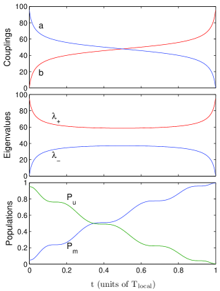
Figure 1: (Color online) Dynamics of the local strategy search for $N=20$ and $\varepsilon=1/11$ (leading to $\alpha T_{\rm local}\approx 96$). Upper frame: $a$ and $b$ (in units of $1/T_{\rm local}$); middle frame: The eigenvalues $\lambda_{\pm}$ (in units of $1/T_{\rm local}$) exhibiting an avoided crossing; lower frame: Populations $P_{u}=|\langle u|\phi\rangle|^{2}$ and $P_{m}=|\langle m|\phi\rangle|^{2}$. The search is achieved with probability 0.995.

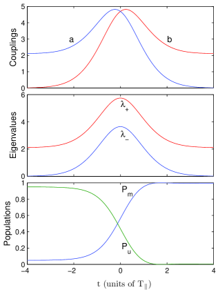
Figure 2: (Color online) Dynamics of the parallel strategy search for $F_{T_{\parallel}}(t)=\tanh(t/T_{\parallel})$, $N=20$ and $\beta T_{\parallel}=4.7$. Upper frame: $a$ and $b$ (in units of $1/T_{\parallel}$); middle frame: The parallel eigenvalues $\lambda_{\pm}$ (in units of $1/T_{\parallel}$); lower frame: Populations $P_{u}=|\langle u|\phi\rangle|^{2}$ and $P_{m}=|\langle m|\phi\rangle|^{2}$. The search is achieved with probability 0.995.

II.3 Parallel strategy

The strategy we propose here consists in following an appropriate level line on the surface of eigenvalues difference as a function of the parameters $a$ and $b$ of the Hamiltonian (3), corresponding to parallel eigenvalues. Let $\frac{2\beta}{\sqrt{N}}$ denote this difference where $\beta$ is some constant to be chosen while, as we shall see below, the $\sqrt{N}$ arises to avoid energy blow up with $N$. From Eq. (4), the level line $\lambda_{+}-\lambda_{-}=\frac{2\beta}{\sqrt{N}}$ is given by the ellipse

$$a^{2}+b^{2}-2ab\left(1-\frac{2}{N}\right)=\frac{\beta^{2}}{N},$$ (20)

or, in canonical form,

$$\frac{(a+b)^{2}}{4\beta^{2}}+\frac{(b-a)^{2}}{\frac{4\beta^{2}}{N-1}}=1.$$ (21)

The initial condition (8), i. e. $b(t_{\rm i})=0$, implied that $a(t_{\rm i})=\frac{2\beta}{\sqrt{N}}$. At the final time $t_{\rm f}$, (9) holds so that $b(t_{\rm f})=\frac{2\beta}{\sqrt{N}}$. It follows that the parametric equation of the ellipse is

$$a(t) = \beta\left(\sqrt{1-\frac{N-1}{N}F^{2}(t)}-\frac{F(t)}{\sqrt{N}}\right)$$

$$b(t) = \beta\left(\sqrt{1-\frac{N-1}{N}F^{2}(t)}+\frac{F(t)}{\sqrt{N}}\right),$$ (22)

with $F(t)$ a strictly monotonous function such that $F(t_{\rm i})=-1$ and $F(t_{\rm f})=1$. Here we consider explicitly the case of the (analytic) hyperbolic tangent of characteristic width $T_{\parallel}$, $F(t)=\tanh(t/T_{\parallel})$. The eigenvalues (4) read here

$$\lambda_{\pm}=\beta\left(\sqrt{1-\frac{N-1}{N}F^{2}(t)}\pm\frac{1}{\sqrt{N}}\right).$$ (23)

Figure 2 displays an example of the dynamics of the search, illustrating how the population transfer is achieved from the prepared state to the marked one. In the numerics, we have truncated the time interval from $t=-4T_{\parallel}$ to $t=4T_{\parallel}$. We have checked that taking a larger interval does not change significantly the result. We have chosen a situation leading to the same efficiency as the local strategy example shown in Fig. 1. Comparing Figs. 1 and 2, one also notices that the search is achieved in an oscillatory manner for the local strategy whereas it is achieved in a monotonic manner for the parallel strategy. This feature, as well as the enhancement of the success rate for the parallel strategy, can be interpreted using superadiabatic basis that are better adapted to describe the dynamics Berry ; Joye . In general, for a strategy using analytic coupling parameters (as considered in the parallel strategy), in the adiabatic limit, the non-adiabatic losses are exponentially small, i.e. of the form $\sim e^{-|\text{const.}|T_{\parallel}}$ and thus beyond any power of $1/T_{\parallel}$ while the corresponding history of the dynamics is smooth and monotonic. For the local strategy, the condition (13) prevents the analyticity of the parameters. The discontinuity of the coupling gives rise to losses which are of order 2 in the off-diagonal elements of (II). More generally, a discontinuity of the $n^{\hbox{\scriptsize th}}$ derivative of the couplings corresponds to polynomial non-adiabatic losses of the order of $(1/T^{n+1})^{2}$, and the corresponding dynamics exhibits oscillations. Indeed, the transformation leading to (II) can be iterated, that is one may further diagonalize (II), which yields higher order derivatives Joye ; Drese . As we show more precisely in the next section, for an identical search cost, the parallel strategy generally enhances the success rate, i. e. reduces the non-adiabatic losses, with respect to the local strategy, or equivalently reduces the cost for an identical success rate.

III Comparison: cost and losses

In order to compare the local and parallel strategies, we shall take into account both the computational cost and the success rate of the search.

III.1 Search cost

In actual implementations, the time-dependent coupling parameters $a(t)$ and $b(t)$ can be achieved, for instance, by laser fields cavity . As a measure of the cost needed to achieve the Grover search we can consider a quantity which is the equivalent of the total laser power. Note that the coupling parameters can either vary significantly during the whole duration of the process (e. g. in the local strategy) or during a small fraction only (e. g. in the parallel strategy). In order to account for both situations, we define the cost $C$ as the product of the peak value $a_{\rm peak}$ of the coupling parameter $a(t)$ and the effective duration of the search $T_{\rm eff}$

$$C=a_{\rm peak}T_{\rm eff},$$ (24)

where $T_{\rm eff}$ is directly related to the characteristic time $T$ of variation of $a(t)$ and is typically a few repetitions of it, $T_{\rm eff}=rT$. Indeed, considering $a(t)$ as a pulse, $T$ is its characteristic width whereas $T_{\rm eff}$ is the full duration for which $a(t)$ is significantly different from its asymptotic $t\rightarrow\pm\infty$ values (hence it can be defined rigorously given some tolerance level). Note that one could define the cost as the area under $a(t)$ for this effective duration. The result would generally differ only by a numerical factor close to one whereas (24) is usually more convenient to compute. For the local strategy, one deduces from (18) that the effective duration $T_{\rm eff}$ corresponds to the whole duration $T_{\rm local}=t_{\rm f}-t_{\rm i}$ given in (17). The cost reads thus

$$C_{\rm local}=\alpha T_{\rm local}=\frac{2\sqrt{N-1}}{\varepsilon}.$$ (25)

For the parallel strategy, we consider analytical functions such as $F(t)=\tanh(t/T_{\parallel})$, which approach their asymptotic values for times $t$ with $|t|\gtrsim rT_{\parallel}/2$. From (22), one obtains the peak value $a_{\rm peak}=\frac{\beta(N-2)}{\sqrt{N(N-1)}}$. Hence, we have

$$C_{\parallel}=\frac{\beta(N-2)}{\sqrt{N(N-1)}}rT_{{\parallel}}\sim\beta rT_{{\parallel}}.$$ (26)

Note that this relation seems to imply that $T_{{\parallel}}$ can be choosen arbitrarily (for instance of order $N^{0}$); However, the non-adiabatic losses, studied below, would then increase dramatically. We shall compare the two strategies at identical costs and then focus our attention below on the success rate of the search. Requiring an identical cost for both strategies yields

$$\beta rT_{{\parallel}}=\frac{2(N-1)\sqrt{N}}{(N-2)\varepsilon}\sim\alpha T_{\rm local}.$$ (27)

For large $N$, the characteristic time of the squared hyperbolic secant, associated with the same cost for both strategies, is thus just $(\alpha/\beta r)\times T_{\rm{local}}$. Moreover, we can require the effective duration of the search to be equal for both strategies which simply amounts to having $\alpha=\beta$. Note that if one chooses $\alpha=\beta=1$, then the search cost is directly equal to the effective search duration. Since there is no loss of generality, we shall assume $\alpha=\beta=1$ throughout.

III.2 Non-adiabatic losses

The success rate of the search is determined by the probability to find the system in the marked state at the final time. This is given by $1-P_{\text{loss}}$ where $P_{\text{loss}}$ corresponds to the probability of the non-adiabatic losses from the instantaneous eigenstate initially populated to the other states. These losses arise because the adiabatic state connected to the initial state is not strictly followed as $\dot{\theta}$ is not strictly zero. For the local strategy, the loss at the final time can be calculated exactly for any $N$. Indeed, the Hamiltonian (II) can be rewritten as

$$H_{\rm ad}=|+\rangle\langle+|+|-\rangle\langle-|+\frac{\lambda_{+}-\lambda_{-}}{2}\left\{|+\rangle\langle+|-|-\rangle\langle-|+i\varepsilon\left(|-\rangle\langle+|-|+\rangle\langle-|\right)\right\},$$ (28)

where $\lambda_{+}-\lambda_{-}$ depends on time according to (19), and use was made of (14) to get $\lambda_{+}+\lambda_{-}=\alpha=1$. Upon extracting the first term which gives rise to a phase and defining a new time $\tau(t)=\int^{t}\frac{\lambda_{+}-\lambda_{-}}{2}dt$ one obtains a stationary Hamiltonian. It follows that, up to a phase, the state of the system at the new time $\tau$ is thus

$$|\psi\rangle(\tau)=\frac{\varepsilon}{\sqrt{1+\varepsilon^{2}}}\sin(\sqrt{1+\varepsilon^{2}}\tau)|-\rangle+\left(\cos(\sqrt{1+\varepsilon^{2}}\tau)-\frac{i}{\sqrt{1+\varepsilon^{2}}}\sin(\sqrt{1+\varepsilon^{2}}\tau)\right)|+\rangle.$$ (29)

From (14), we deduce that at the end of the process, $\tau(t_{\rm f})=\frac{1}{\varepsilon}\arctan\sqrt{N-1}$. The non-adiabatic losses are therefore

$$P_{\text{loss,local}}=\frac{\varepsilon^{2}}{1+\varepsilon^{2}}\sin^{2}\left(\frac{\sqrt{1+\varepsilon^{2}}}{\varepsilon}\arctan\sqrt{N-1}\right),$$ (30)

i.e., in the limit of large $N$ and small $\varepsilon$

$$P_{\text{loss,local}}\sim\varepsilon^{2}\sin^{2}\left(\frac{\pi}{2\varepsilon}\right).$$ (31)

Note that the choice of the specific values $\varepsilon=1/2p$ with an integer $p$ will give losses going to 0 for large $N$. However these choices of specific and thus non-robust values will not be considered here since they are outside the adiabatic scope. A good measure of the losses is the upper boundary $\varepsilon^{2}$. The adiabatic regime for the local strategy is thus reached when $\varepsilon\ll 1$, i.e., using (17), when

$$\frac{T_{\text{local}}}{\sqrt{N}}=\frac{2}{\varepsilon}\gg 1\qquad N\gg 1.$$ (32)

For the level line optimization, it has been shown in Ref. Leveline that the adiabatic regime is obtained when $T_{\parallel}(\lambda_{+}-\lambda_{-})=2T_{\parallel}/\sqrt{N}\gg 1$. Actually, for $F(t)=\tanh(t/T_{\parallel})$, we can calculate the non-adiabatic losses for large $N$,

$$P_{\text{loss, $\parallel$}}\sim\text{sech}^{2}\left(\frac{\pi T_{\parallel}\beta}{\sqrt{N}}\right).$$ (33)

This result comes from the fact that, for $N\gg 1$, the model (3) corresponds, up to a phase, to the Allen-Eberly model AE . Equation (33) shows the $\sqrt{N}$ scaling of the search cost since taking $T_{\parallel}$ growing as $\sqrt{N}$,

$$\frac{T_{\parallel}}{\sqrt{N}}\equiv\frac{1}{\gamma}\gg 1\qquad N\gg 1,$$ (34)

allows one to obtain the same arbitrarily small non-adiabatic losses for any $N$,

$$P_{\text{loss,$\parallel$}}\sim\text{sech}^{2}\left(\frac{\pi}{\gamma}\right)\sim 4\exp\left(-\frac{2\pi}{\gamma}\right).$$ (35)

Requesting the same cost for both strategies, we deduce from (27), (32) and (34)

$$\gamma\sim\frac{\varepsilon r}{2}.$$ (36)

The losses (35), being of the form $e^{-2\pi/\gamma}$, are beyond any power of $1/\gamma$, and are thus expected to be much smaller than the ones given by the local strategy which are of order $\varepsilon^{2}$.

IV Numerical illustration

The quadratic speedup of the search using the parallel strategy was derived on the basis of the asymptotic result (33) obtained for large $N$. We first show that the losses are also well approximated by (33) for finite $N$. In Fig. 3 we plot the non-adiabatic losses obtained numerically as a function of $1/\gamma$ defined as $T_{\parallel}/\sqrt{N}$. The case $N=20$ (oscillating full line) is close to the asymptotic result (non-oscillating one) which, as expected from (33), shows a strong exponential decay. The search is efficient for $1/\gamma\geq 1$, with for instance $P_{\text{loss, $\parallel$}}\sim 10^{-2}$ for $\gamma=1$. Similar results hold for other values of $N$.

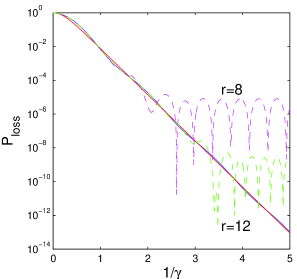
Figure 3: (Color online) Final losses (in logarithmic scale) as a function of $1/\gamma=T_{{\parallel}}/\sqrt{N}$ (dimensionless) for $N=20$ with $F(t)=\tanh(t/T_{\parallel})$ (oscillating full line) its asymptotic value given by (33) (non-oscillating full line, almost undistinguishable from the oscillating full line), and for truncated time domains $r=12$ and $r=8$ (dashed lines).

In contrast to the local strategy, the parallel strategy uses analytical couplings on an unbounded domain. Hence, in practice one has to truncate this domain to limit the time of search. This truncation of the couplings, breaking the continuity, leads in general to additional non-adiabatic losses. In Sec. III.1 we defined the finite domain through the quantity $r$ as $T_{\text{eff}}=rT_{\parallel}$. Figure 3 shows the losses for $r=8$ and $r=12$. As expected, the loss becomes larger for smaller $r$ when decreasing $\gamma$. For $r=12$, the range of validity of the asymptotic formula (35) is approximately $1/\gamma\lesssim 3$. This means that up to $1/\gamma\sim 3$ the additional losses due to the truncation can be neglected (otherwise, one could take a larger value for $r$).

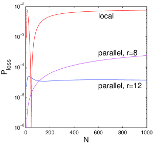
Figure 4: (Color online) Final losses as a function of $N$ for $\varepsilon=1/11$ for the local strategy and for the parallel strategy with $F(t)=\tanh(t/T_{\parallel})$ with a truncated time intervals ($r=12$ and $r=8$) and $\gamma$ given by Eq. (36) to have the same cost.

Figure 4 depicts the losses as a function of $N$ for a given value of $\varepsilon$ and the corresponding value of $\gamma$ given by (36) with two truncations $r=8$ and $r=12$. This figure shows that the parallel strategy is more efficient, as expected from the comparison of (32) and (34) with (36), despite the truncation of the time interval which breaks the analyticity of the coupling. Note, however, that a truncation with too small a value for $r$ can lead to a significant dependance of the losses with $N$.

V Conclusion

We have proposed a strategy to achieve the Grover search by adiabatic passage using parallel eigenvalues. We have compared this parallel strategy with the known local strategy which requires an adaptation of the speed of the dynamics with respect to the given dynamical gap between the eigenvalues. We have shown the superiority of the parallel strategy: for an identical search cost, the parallel strategy enhances the success rate with respect to the local strategy, i. e. reduces the non-adiabatic losses, or equivalently reduces the cost for an identical success rate. Smooth analytic coupling parameters are in principle required for the parallel strategy. We have however shown numerically that a truncation of the time domain, which is necessary in practice, preserves the higher efficiency of the success rate of the search at identical cost. We have here used an hyperbolic tangent for $F(t)$ since it allows one to determine analytically the population dynamics for large $N$. We have checked that other similar shapes for $F(t)$, for instance associated to Gaussians which are easily performed in the laboratory, preserves the advantage of the parallel strategy over the local one.

References

- (1) E. Farhi, J. Goldstone, S. Gutmann, and M. Sipser, e-print quant-ph/0001106.
- (2) A. M. Childs, E. Farhi, and J. Preskill, Phys. Rev. A 65, 012322 (2001).
- (3) M. A. Nielsen and I. L. Chuang, Quantum Computation and Quantum Information, Cambridge University Press, Cambridge, 2000.
- (4) E. Farhi and S. Gutmann, Phys. Rev. A 57, 2403 (1998).
- (5) J. Roland and N. J. Cerf, Phys. Rev. A 65, 042308 (2002).
- (6) S. Guérin, S. Thomas and H. R. Jauslin, Phys. Rev. A 65, 023409 (2002).
- (7) S. Guérin and H. R. Jauslin, Adv. Chem. Phys. 125, 147 (2003).
- (8) M. V. Berry, Proc. Roy. Soc. Lond. A 429, 61 (1990).
- (9) A. Joye, C.-E. Pfister, J. Math. Phys. 34, 454 (1993).
- (10) K. Drese and M. Holthaus, Eur. Phys. J. D 3, 73-86 (1998).
- (11) D. Daems and S. Guérin, Phys. Rev. Lett. 99, 170503 (2007); Phys. Rev. A 78, 022330 (2008).
- (12) L. Allen and J. H. Eberly, Optical Resonance and Two-Level Atoms (Dover, New York, 1987).