Changing the mechanical unfolding pathway
of FnIII₁₀ by tuning the pulling strength

We investigate the mechanical unfolding of the tenth type III domain from fibronectin, FnIII₁₀, both at constant force and at constant pulling velocity, by all-atom Monte Carlo simulations. We observe both apparent two-state unfolding and several unfolding pathways involving one of three major, mutually exclusive intermediate states. All the three major intermediates lack two of seven native $\beta$-strands, and share a quite similar extension. The unfolding behavior is found to depend strongly on the pulling conditions. In particular, we observe large variations in the relative frequencies of occurrence for the intermediates. At low constant force or low constant velocity, all the three major intermediates occur with a significant frequency. At high constant force or high constant velocity, one of them, with the N- and C-terminal $\beta$-strands detached, dominates over the other two. Using the extended Jarzynski equality, we also estimate the equilibrium free-energy landscape, calculated as a function of chain extension. The application of a constant pulling force leads to a free-energy profile with three major local minima. Two of these correspond to the native and fully unfolded states, respectively, whereas the third one can be associated with the major unfolding intermediates.

 
^∗Computational Biology & Biological Physics, Department of Theoretical Physics, Lund University, Lund, Sweden. ^†Istituto dei Sistemi Complessi, CNR, Sesto Fiorentino, Italy; INFN Sezione di Firenze, Sesto Fiorentino, Italy. ^‡ISI Foundation, Torino, Italy. ^§Present address: Department of Physics and Astronomy, University of Aarhus, Denmark.

Corresponding author: Simon Mitternacht, tel: +46-46-2223494,
    fax: +46-46-2229686, e-mail: simon@thep.lu.se

Running title: Mechanical unfolding of FnIII₁₀

Key words: force-induced unfolding, all-atom model, Monte Carlo, Jarzynski’s equality.

Fibronectin is a giant multimodular protein that exists in both soluble (dimeric) and fibrillar forms. In its fibrillar form, it plays a central role in cell adhesion to the extracellular matrix. Increasing evidence indicates that mechanical forces exerted by cells are a key player in initiation of fibronectin fibrillogenesis as well as in modulation of cell-fibronectin adhesion, and thus may regulate the form and function of fibronectin [1, 2].

Each fibronectin monomer contains more than 20 modules of three types, called FnI–III. The most common type is FnIII, with $\sim$90 amino acids and a $\beta$-sandwich fold. Two critical sites for the interaction between cells and fibronectin are the RGD motif Arg78-Gly79-Asp80 [3] on the tenth FnIII module, FnIII₁₀, and a synergistic site [4] on the ninth FnIII module, which bind to cell-surface integrins. In the native structure of FnIII₁₀, shown in Fig. 1, the RGD motif is found on the loop connecting the C-terminal $\beta$-strands F and G. It has been suggested that a stretching force can change the distance between these two binding sites sufficiently to affect the cell-adhesion properties, without deforming the sites themselves [2]. Force could also influence the adhesion properties by causing full or partial unfolding of the FnIII₁₀ module, and thereby deformation of the RGD motif [5]. Whether or not mechanical unfolding of fibronectin modules occurs in vivo is controversial. It is known that cell-generated force can extend fibronectin fibrils to several times their unstretched length [6]. There are experiments indicating that this extensibility is due to changes in quaternary structure rather than unfolding [7], while other experiments indicate that the extensibility originates from force-induced unfolding of FnIII modules [8, 9]. Also worth noting is that the FnIII₁₀ module is capable of fast refolding [10].

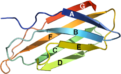
Figure 1: Schematic illustration of the NMR-derived [53] native structure of FnIII₁₀ (Protein Data Bank ID 1ttf). Its seven $\beta$-strands are labeled A–G in sequence order.

Atomic force microscopy (AFM) experiments have provided important insights into the mechanical properties of FnIII modules [11, 12, 13]. Interestingly, it was found that, although thermodynamically very stable [14], the cell-binding module FnIII₁₀ is mechanically one of the least stable FnIII modules [11]. Further, it was shown that the force-induced unfolding of FnIII₁₀ often occurs through intermediate states [12]. While apparent one-step events were seen as well, a majority of the unfolding events had a clear two-step character [12]. A recent AFM study of pH dependence [13] suggests that electrostatic contributions are less important for the mechanical stability of FnIII₁₀ than previously thought.

Several groups have used computer simulations to investigate the force-induced unfolding of FnIII₁₀ [5, 15, 16, 17, 18, 19, 20]. An early study predicted the occurrence of intermediate states [15]. In these simulations, two unfolding pathways were seen, both proceeding through partially unfolded intermediate states. Both intermediates lacked two of the seven native $\beta$-strands. The missing strands were A and B in one case, and A and G in the other (for strand labels, see Fig. 1). A more recent study reached somewhat different conclusions [17]. This study found three different pathways, only one of which involved a partially unfolded intermediate state, with strands A and B detached. The experiments [12] are consistent with the existence of the two different intermediates seen in the early simulations [15], but do not permit an unambiguous identification of the states. When comparing the experiments with these simulations, it should be kept in mind that the forces studied in the simulations were larger than those studied experimentally.

Here we use an implicit-water all-atom model with a simple and computationally convenient energy function [21, 22] to investigate how the response of FnIII₁₀ to a stretching force depends on the pulling strength. We study the unfolding behavior both at constant force and at constant pulling velocity. Some previous studies were carried out using explicit-solvent models [5, 17, 18]. These models might capture important details that our implicit-solvent model ignores, like weakening of specific hydrogen bonds through interactions between water molecules and the protein backbone [23]. The advantage of our model is computational convenience. The relative simplicity of the model makes it possible for us to generate a large set of unfolding events, which is important when studying a system with multiple unfolding pathways.

Our analysis of the generated unfolding trajectories consists of two parts. The first part aims at characterizing the major unfolding pathways and unfolding intermediates. In the second part, we use the extended Jarzynski equality (EJE) [24, 25, 26] to estimate the equilibrium free-energy landscape, calculated as a function of end-to-end distance. This analysis extends previous work on simplified protein models [27, 28, 29, 30] to an atomic-level model. This level of detail may be needed to facilitate comparisons with future EJE reconstructions based on experimental data. Indeed, two applications of this method to experimental protein data were recently reported [31, 32].

Model and Methods

Model

We use an all-atom model with implicit water, torsional degrees of freedom, and a simplified energy function [21, 22]. The energy function

$$E=E_{\text{loc}}+E_{\text{ev}}+E_{\text{hb}}+E_{\text{hp}}$$ (1)

is composed of four terms. The term $E_{\text{loc}}$ is local in sequence and represents an electrostatic interaction between adjacent peptide units along the chain. The other three terms are non-local in sequence. The excluded volume term $E_{\text{ev}}$ is a $1/r^{12}$ repulsion between pairs of atoms. $E_{\mathrm{hb}}$ represents two kinds of hydrogen bonds: backbone-backbone bonds and bonds between charged side chains and the backbone. The last term $E_{\text{hp}}$ represents an effective hydrophobic attraction between nonpolar side chains. It is a simple pairwise additive potential based on the degree of contact between two nonpolar side chains. The precise form of the different interaction terms and the numerical values of all geometry parameters can be found elsewhere [21, 22].

It has been shown that this model, despite its simplicity, provides a good description of the structure and folding thermodynamics of several peptides with different native geometries [22]. For the significantly larger protein FnIII₁₀, it is computationally infeasible to verify that the native structure is the global free-energy minimum. However, in order to study unfolding, it is sufficient that the native state is a local free-energy minimum. In our model, with unchanged parameters [21, 22], the native state of FnIII₁₀, indeed, is a long-lived state corresponding to a free-energy minimum, as will be seen below.

The same model has previously been used to study both mechanical and thermal unfolding of ubiquitin [33, 34]. In agreement with AFM experiments [35], it was found that ubiquitin, like FnIII₁₀, displays a mechanical unfolding intermediate far from the native state, and this intermediate was characterized [33]. The picture emerging from this study [33] was subsequently supported by ubiquitin simulations based on completely different models [36, 37, 38].

The energy function $E$ of Eq. 1 describes an unstretched protein. In our calculations, the protein is pulled either by a constant force or with a constant velocity. In the first case, constant forces $-\vec{F}$ and $\vec{F}$ act on the N and C termini, respectively. The full energy function is then given by

$$E_{\text{tot}}=E-\vec{F}\cdot\vec{R}$$ (2)

where $\vec{R}$ is the vector from the N to the C terminus. In the constant-velocity simulations, the pulling of the protein is modeled using a harmonic potential in the end-to-end distance $L=|\vec{R}|$ whose minimum $L_{v}(t)$ varies linearly with Monte Carlo (MC) time $t$. With this external potential, the full, time-dependent energy function becomes

$$E_{\text{tot}}(t)=E+\frac{k}{2}\left[L_{v}(t)-L\right]^{2}=E+\frac{k}{2}\left[L_{0}+vt-L\right]^{2}$$ (3)

where $k$ is a spring constant, $v$ is the pulling velocity, and $L_{0}$ is the initial equilibrium position of the spring. The spring constant, corresponding to the cantilever stiffness in AFM experiments, is set to $k=37$ pN/nm. The experimental FnIII₁₀ study of [12] reported a typical spring constant of $k\sim 50$ pN/nm.

Simulation methods

Using MC dynamics, we study six constant force magnitudes $F$ (50 pN, 80 pN, 100 pN, 120 pN, 150 pN and 192 pN) and four constant pulling velocities $v$ (0.03 fm/MC step, 0.05 fm/ MC step, 0.10 fm/MC step and 1.0 fm/MC step), at a temperature of 288 K. Three different types of MC updates are used: (i) Biased Gaussian Steps [39], BGS, which are semi-local updates of backbone angles; (ii) single-variable Metropolis updates of side-chain angles; and (iii) small rigid-body rotations of the whole chain. The BGS move simultaneously updates up to eight consecutive backbone angles, in a manner that keeps the chain ends approximately fixed. In the constant-velocity simulations, the time-dependent parameter $L_{v}(t)$ is changed after every attempted MC step.

As a starting point for our simulations, we use a model approximation of the experimental FnIII₁₀ structure (backbone root-mean-square deviation $\approx$ 0.2 nm), obtained by simulated annealing. All simulations are started from this initial structure, with different random number seeds. However, in the constant-velocity runs, the system is first thermalized in the potential $E+k(L_{0}-L)^{2}/2$ for $10^{7}$ MC steps ($L_{0}=3.8$ nm), before the actual simulation is started at $t=0$. The thermalization is a prerequisite for the Jarzynski analysis (see below).

The constant-force simulations are run for a fixed time, which depends on the force magnitude. There are runs in which the protein remains folded over the whole time interval studied. The constant-velocity simulations are run until the spring has been pulled a distance of $vt=35$ nm. At this point, the protein is always unfolded.

Our simulations are carried out using the program package PROFASI [40], which is a C++ implementation of this model. 3D structures are drawn with PyMOL [41].

Analysis of pathways and intermediates

To characterize pathways and intermediates, we study the evolution of the native secondary-structure elements along the unfolding trajectories. For this purpose, during the course of the simulations, all native hydrogen bonds connecting two $\beta$-strands (see Fig. 1) are monitored. A bond is defined as present if the energy of that bond is lower than a cutoff ($-2.4k_{\text{B}}T$). Using this data, we can describe a configuration by which pairs of $\beta$-strands are formed. A $\beta$-strand pair is said to be formed if more than a fraction 0.3 of its native hydrogen bonds are present. Whether individual $\beta$-strands are present or absent is determined based on which $\beta$-strand pairs the conformation contains.

The characterization of intermediate states requires slightly different procedures in the respective cases of constant force and constant velocity. For constant force, a histogram of the end-to-end distance $L$, covering the interval $3\,\textrm{nm}<L<27\,\textrm{nm}$, is made for each unfolding trajectory. Each peak in the histogram corresponds to a metastable state along the unfolding pathway. To reduce noise the histogram is smoothed with a sliding $L$ window of 0.3 nm. Peaks higher than a given cutoff are identified. Two peaks that are close to each other are only considered separate states if the values between them drop below half the height of the smallest peak. The position of an intermediate, $L_{\text{I}}$, is calculated as a weighted mean over the corresponding peak. The area under the peak provides, in principle, a measure, $\tau_{\text{I}}$, of the life time of the state. However, due to statistical difficulties, we do not measure average life times of intermediate states.

In the constant-velocity runs, the unraveling of the native state or an intermediate state is associated with a rupture event, at which a large drop in force occurs. To ascertain that we register actual rupture events and not fluctuations due to thermal noise, the force versus time curves are smoothed with a sliding time window of $T_{\text{w}}=0.3\,\textrm{nm}/v$, where $v$ is the pulling velocity. Rupture events are identified as drops in force that are larger than 25 pN within a time less than $T_{\text{w}}$. The point of highest force just before the drop defines the rupture force, $F_{\text{I}}$, and the end-to-end distance, $L_{\text{I}}$, of the corresponding state. Only rupture events with a time separation of at least $2T_{\text{w}}$ are considered separate events. The rupture force $F_{\text{I}}$ is a stability measure statistically easier to estimate than the life time $\tau_{\text{I}}$ at constant force.

For a peak with a given $L_{\text{I}}$, to decide which $\beta$-strands the corresponding state contains, we consider all stored configurations with $|L-L_{\text{I}}|<0.1$ nm. All $\beta$-strand pairs occurring at least once in these configurations are considered formed in the state. With this prescription, it happens that separate peaks from a single run exhibit the same set of $\beta$-strand pairs. Distinguishing between different substates with the same secondary-structure elements is beyond the scope of the present work. Such peaks are counted as a single state, with $L_{\text{I}}$ set to the weighted average position of the merged peaks.

Jarzynski analysis

From the constant-velocity trajectories, we estimate the equilibrium free-energy landscape $G_{0}(L)$, as a function of the end-to-end distance $L$, for the unstretched protein by using EJE [24, 25, 26, 42]. For our system, this identity takes the form

$$\textrm{e}^{-G_{0}(L)/k_{\text{B}}T}=\textrm{constant}\cdot\textrm{e}^{k[L-L_{v}(t)]^{2}/2k_{\text{B}}T}\times\\ \langle\delta(L-L(C_{t}))\textrm{e}^{-W_{t}/k_{\text{B}}T}\rangle_{t}$$ (4)

where $k_{\text{B}}$ is Boltzmann’s constant, $T$ the temperature, and $C_{t}$ stands for the configuration of the system at time $t$. In this equation, $\langle\ldots\rangle_{t}$ denotes an average over trajectories $C_{\tau}$, $0<\tau<t$, with starting points $C_{0}$ drawn from the Boltzmann distribution corresponding to $E_{\text{tot}}(0)$ (see Eq. 3). The quantity $W_{t}$ is the work done on the system along a trajectory and is given by

$$W_{t}=\int_{0}^{t}kv[L_{v}(\tau)-L(C_{\tau})]\,\text{d}\tau=\int F\,\text{d}L_{v}$$ (5)

As discussed in [26, 42], combining Eq. 4 with the weighted histogram method [43], one finds that the optimal estimate of the target function $G_{0}(L)$ is given by

$$G_{0}(L)=\\ -k_{\text{B}}T\ln\left[\frac{\sum_{t}\langle\delta(L-L(C_{t}))\textrm{e}^{-W_{t}/k_{\text{B}}T}\rangle_{t}/\langle\textrm{e}^{-W_{t}/k_{\text{B}}T}\rangle}{\sum_{t}\textrm{e}^{-k[L-L_{v}(t)]^{2}/2k_{\text{B}}T}/\langle\textrm{e}^{-W_{t}/k_{\text{B}}T}\rangle}\right],$$ (6)

up to an additive constant. As in an experimental situation, for each unfolding trajectory, we sample the end-to-end distance $L(C_{t})$ and the work $W_{t}$ at discrete time intervals $k\Delta\tau$, with $k=0,\dots,n$ and $n\Delta\tau=t$. The sums appearing in Eq. 6 thus run over these discrete times.

Let $L_{\min}$ and $L_{\max}$ be the minimal and maximal end-to-end distances, respectively, observed in the unfolding trajectories. We divide the interval $\left[L_{\min},L_{\max}\right]$ into sub-intervals of length $\Delta L$ and evaluate $G_{0}(L_{i})$ for each $L_{i}=L_{\min}+(i+1/2)\Delta L$ by exploiting Eq. 6. The two averages appearing in this equation are estimated as $\overline{\theta_{i}(L(C_{t}))\exp(-W_{t}/k_{\text{B}}T)}$ and $\overline{\exp(-W_{t}/k_{\text{B}}T)}$, where the bar indicates an average over trajectories and the function $\theta_{i}(x)$ is defined as $\theta_{i}(x)=1$ if $|x-L_{i}|<\Delta L/2$ and $\theta_{i}(x)=0$ otherwise. Further details on the scheme used can be found in [42].

Results

Description of the calculated unfolding traces

We study the mechanical unfolding of FnIII₁₀ for six constant forces and four constant velocities. Table 1 shows the number of runs and the length of each run in these ten cases. At low force or low velocity, it takes longer for the protein to unfold, which makes it necessary to use longer and computationally more expensive trajectories.

pulling force or velocity	runs	MC steps/$10^{6}$
50 pN	98	1 000
80 pN	100	1 000
100 pN	100	250
120 pN	200	100
150 pN	340	50
192 pN	600	30
0.03 fm$/$MC step	100	1 167
0.05 fm$/$MC step	99	700
0.10 fm$/$MC step	99	350
1.0 fm$/$MC step	200	35

Table 1: Number of runs and the length of each run, in number of elementary MC steps, at the different pulling conditions studied.

Fig. 2 shows the time evolution of the end-to-end distance $L$ in a representative set of runs at constant force (100 pN). Typically each trajectory starts with a long waiting phase with $L\sim 5$ nm, where the molecule stays close to the native conformation. In this phase, the relative orientation of the two $\beta$-sheets (see Fig.1) might change, but all native $\beta$-strands remain unbroken. The waiting phase is followed by a sudden increase in $L$. This step typically leads either directly to the completely unfolded state with $L\sim 30$ nm or, more commonly, to an intermediate state at $L\sim 12$–16 nm. The intermediate is in turn unfolded in another abrupt step that leads to the completely stretched state. In a small fraction of the trajectories, depending on force, the protein is still in the native state or an intermediate state when the simulation stops. Intermediates outside the range 12–16 nm are unusual but occur in some runs. For example, a relatively long-lived intermediate at 21 nm can be seen in one of the runs in Fig. 2.

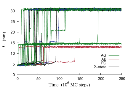
Figure 2: MC time evolution of the end-to-end distance in 42 independent simulations with a constant pulling force of 100 pN. The three most frequent intermediates lack different pairs of native $\beta$-strands: AG, FG, or AB. Trajectories in which these states occur are labeled green, blue and red, respectively. Apparent two-state events are colored black.

Fig. 3 shows samples of unfolding traces at constant velocity (0.05 fm/MC step). Here force is plotted against end-to-end distance. As in the constant-force runs, there are two main events in most trajectories. First, the native state is pulled until it ruptures at $L\sim 5$ nm. The chain is then elongated without much resistance until it, in most cases, reaches an intermediate at $L\sim 12$–16 nm. Here the force increases until there is a second rupture event. After that, the molecule is free to elongate towards the fully unfolded state with $L\sim 30$ nm. Some trajectories have force peaks at other $L$. An unusually large peak of this kind can be seen at 22 nm in Fig. 3. Inspection of the corresponding structure reveals that it contains a three-stranded $\beta$-sheet composed of the native CD hairpin and a non-native strand. This sheet is pulled longitudinally, which explains why the stability is high. Another feature worth noting in Fig. 3 is that the pulling velocity is sufficiently small to permit the force to drop to small values between the peaks.

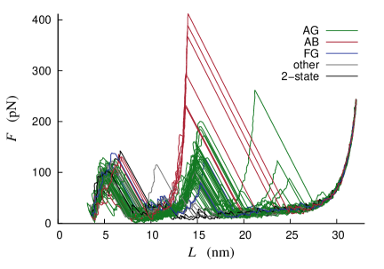
Figure 3: Force versus end-to-end distance in 55 independent simulations with a constant pulling velocity of $0.05$ fm/MC step. Noise has been filtered out using a sliding time window of $6\cdot 10^{6}$ MC steps. The color coding is the same as in Fig. 2, with the addition of a new category for a few trajectories not belonging to any of the four categories in that figure. These trajectories are colored grey.

There are several similarities between the unfolding events seen at constant force and at constant velocity. In most trajectories, there are stable intermediates, and the unfolding from both the native and intermediate states is abrupt. Also, the vast majority of the observed intermediates have a similar end-to-end distance, in the range 12–16 nm. It should be noticed that experiments typically measure contour-length differences rather than end-to-end distances. Below we analyze contour-length differences between the native state and our calculated intermediates, which turn out to be in good agreement with experimental data.

The trajectories can be divided into three categories: apparent two-state unfolding, unfolding through intermediate states, and trajectories in which no unfolding takes place. Table 2 shows the relative frequencies of these groups at the different pulling conditions. The number of trajectories in which the protein remains folded throughout the run obviously depends on the trajectory length. More interesting to analyze is the ratio between the two kinds of unfolding, with or without intermediate states. In the constant-force runs, this ratio depends strongly on the magnitude of the applied force; unfolding through intermediates dominates at the lowest force, but is less common than apparent two-state unfolding at the highest force. In the constant-velocity runs, unfolding through intermediates is much more probable than apparent two-state unfolding at all the velocities studied.

pulling force or velocity	$n=2$	$n\geq 3$	no unfolding
50 pN	0.01	0.79	0.20
80 pN	0.21	0.79	0
100 pN	0.23	0.77	0
120 pN	0.24	0.76	0
150 pN	0.29	0.72	$<$0.01
192 pN	0.54	0.46	0
0.03 fm/MC step	0.04	0.96	0
0.05 fm/MC step	0.07	0.93	0
0.10 fm/MC step	0.03	0.97	0
1.0 fm/MC step	0	1.0	0

Table 2: The fractions of trajectories in which unfolding occurs either in an apparent two-state manner (labeled $n=2$) or through intermediate states (labeled $n\geq 3$). “No unfolding” refers to the fraction of trajectories in which the protein remains folded throughout the run (with $L<8$ nm).

Identifying pathways and intermediates

The fact that most observed intermediates fall in the relatively narrow $L$ interval of 12–16 nm does not mean that they are structurally similar. Actually, the data in Figs. 2 and 3 clearly indicate that these intermediates can be divided into three groups with similar but not identical end-to-end distances. The $\beta$-strand analysis (see Model and Methods) reveals that these three groups correspond to the detachment of different pairs of $\beta$-strands, namely A and G, A and B, or F and G. The prevalence of these particular intermediate states is not surprising, given the native topology. When pulling the native structure of FnIII₁₀, the interior of the molecule is shielded from force by the N- and C-terminal $\beta$-strands, A and G. Consequently, in 95 % or more of our runs, either strand A or G is the first to detach, for all the pulling conditions studied. Most commonly, this detachment is followed by a release of the other strand of the two. But, when A (G) is detached, B (F) is also exposed to force. We thus have three main options for detaching two strands, AG, AB or FG, which actually correspond to the three major intermediates we observe.

Intermediates outside the interval 12–16 nm also occur in our simulations. When applied to the intermediates with $L<12$ nm, the $\beta$-strand analysis identifies two states with one strand detached, A or G. The intermediates with $L>16$ nm are scattered in $L$ and correspond to rare states with more than two strands detached. The intermediate at 21 nm seen in one of the runs in Fig. 2 lacks, for example, four strands (A, B, F and G). However, in these relatively unstructured states with more than two strands detached, the remaining strands are often disrupted, which makes the binary classification of strands as either present or absent somewhat ambiguous. Moreover, it is not uncommon that these large-$L$ intermediates contain some non-native secondary structure. In what follows, we therefore focus on the five states seen with only one or two strands detached.

For convenience, the intermediates will be referred to by which strands are detached. The intermediate with strands A and B unfolded will thus be labeled AB, etc. Tables 3 and 4 show basic properties of the A, G, AB, AG and FG intermediates, as observed at constant force and constant velocity, respectively.

	50 pN		80 pN		100 pN		120 pN		150 pN		192 pN
state	$f$	$\bar{L}_{\text{I}}$	$f$	$\bar{L}_{\text{I}}$	$f$	$\bar{L}_{\text{I}}$	$f$	$\bar{L}_{\text{I}}$	$f$	$\bar{L}_{\text{I}}$	$f$	$\bar{L}_{\text{I}}$
AG	0.46	13.9	0.49	14.3	0.65	14.3	0.69	14.5	0.69	14.6	0.45	14.7
AB	0.35	12.4	0.14	12.9	0.09	13.1	0.03	13.2	$<$0.01	—	$<$0.01	—
FG	0.15	14.8	0.13	15.2	0.03	15.5	0.03	15.7	$<$0.01	—	$<$0.01	—
G	0.19	11.1	0.04	11.8	0	—	0	—	0	—	0	—
A	0.13	6.7	0	—	0	—	0	—	0	—	0	—

Table 3: Frequency $f$ and average extension $\bar{L}_{\text{I}}$ (in nm) of intermediate states in the constant-force simulations. The label of a state indicates which $\beta$-strands are detached, that is the state AG lacks strands A and G, etc. The frequency $f$ is the number of runs in which a given state was seen, divided by the total number of runs in which unfolding occurred. The statistical uncertainties on $\bar{L}_{\text{I}}$ are about 0.1 nm or smaller. “—” indicates not applicable.

	0.03 fm$/$MC step			0.05 fm$/$MC step			0.10 fm$/$MC step			1.0 fm$/$MC step
state	$f$	$\bar{F}_{\text{I}}$	$\bar{L}_{\text{I}}$	$f$	$\bar{F}_{\text{I}}$	$\bar{L}_{\text{I}}$	$f$	$\bar{F}_{\text{I}}$	$\bar{L}_{\text{I}}$	$f$	$\bar{F}_{\text{I}}$	$\bar{L}_{\text{I}}$
AG	0.60	115	14.9	0.69	121	14.9	0.78	131	14.8	0.81	198	15.0
AB	0.14	283	13.7	0.09	289	13.8	0.08	333	13.9	0.04	318	13.9
FG	0.15	119	15.6	0.08	107	15.3	0.08	162	16.0	0.04	216	15.7
G	0.05	54	10.5	0.08	73	10.8	0.20	46	9.9	0.06	67	10.3
A	0.06	43	6.2	0.07	53	7.2	0.09	57	6.9	0.03	81	7.2

Table 4: Frequency $f$, average rupture force $\bar{F}_{\text{I}}$ (in pN) and average extension $\bar{L}_{\text{I}}$ (in nm) of intermediate states in the constant-velocity simulations. The statistical uncertainties are 10–20 % on $F_{\text{I}}$, about 0.1 nm or smaller on $L_{\text{I}}$ for AG and AB, and about 0.5 nm on $L_{\text{I}}$ for FG, G and A.

From Tables 3 and 4, several observations can be made. A first one is that the average end-to-end distance, $\bar{L}_{\text{I}}$, of a given state increases slightly with increasing force. More importantly, it can be seen that the relative frequencies with which the different intermediates occur depend strongly on the pulling conditions. At high force or high velocity, the AG intermediate stands out as the by far most common one. By contrast, at low force or low velocity, there is no single dominant state. In fact, at $F=50$ pN as well as at $v=0.03$ fm/MC step, all the five states occur with a significant frequency.

Table 4 also shows the average rupture force, $\bar{F}_{\text{I}}$, of the different states, at the different pulling velocities. Although the data are somewhat noisy, there is a clear tendency that $\bar{F}_{\text{I}}$, for a given state, slowly increases with increasing pulling velocity, which is in line with the expected logarithmic $v$ dependence [44]. Comparing the different states, we find that those with only one strand detached (A and G) are markedly weaker than those with two strands detached (AG, AB and FG), as will be further discussed below. Most force-resistant is the AB intermediate. This state occurs much less frequently than the AG intermediate, especially at high velocity, but is harder to break once formed. Compared to experimental data, our $\bar{F}_{\text{I}}$ values for the intermediates are somewhat large. The experiments found a relatively wide distribution of unfolding forces centered at 40–50 pN [12], which is a factor two or more lower than what we find for the AG, AB and FG intermediates. Our results for the unfolding force of the native state are consistent with experimental data. For the native state, the experiments found unfolding forces of $75\pm 20$ pN [11] and $90\pm 20$ pN [12]. Our corresponding results are $88\pm 2$ pN, $99\pm 2$ pN and $114\pm 3$ pN at $v=0.03$ fm/MC step, $v=0.05$ fm/MC step and $v=0.10$ fm/MC step, respectively.

The AG, AB and FG intermediates do not only require a significant rupture force in our constant-velocity runs, but are also long-lived in our constant-force simulations. In fact, in many runs, the system is still in one of these states when the simulation ends, which means that their average life times, unfortunately, are too long to be determined from the present set of simulations. Nevertheless, there is a clear trend that the AB intermediate is more long-lived than the other two, which in turn have similar life times. The relative life times of these states in the constant-force runs are thus fully consistent with their force-resistance in the constant-velocity runs.

At high constant force, we see a single dominant intermediate, the AG state, but also a large fraction of events without any detectable intermediate. Interestingly, it turns out that the same two strands, A and G, are almost always the first to break in the apparent two-state events as well. Table 5 shows the fraction of all trajectories, with or without intermediates, in which A and G are the first two strands to break, at the different forces studied. At 192 pN, this fraction is as large as 98 %. Although the time spent in the state with strands A and G detached varies from run to run, there is thus an essentially deterministic component in the simulated events at high force.

​first pair	50 pN	80 pN	100 pN	120 pN	150 pN	192 pN
A & G	0.50	0.69	0.87	0.935	0.973	0.980
A & B	0.35	0.15	0.09	0.025	0.006	0.007
F & G	0.15	0.16	0.04	0.040	0.021	0.013

Table 5: The fractions of all unfolding events in which the first two strands to break are A & G, F & G, and A & B, respectively, at different constant forces. The first pair to break was always one of these three.

The unfolding behavior at low force or velocity is, by contrast, complex, with several possible pathways. Fig. 4 illustrates the relations between observed pathways at the lowest pulling velocity, 0.03 fm/MC step. The main unfolding path begins with the detachment of strand G, followed by the formation of the AG intermediate, through the detachment of A. There are also runs in which the same intermediate occurs but A and G detach in the opposite order. Note that for the majority of the trajectories the boxes A and G in Fig. 4 only indicate passage through these states, not the formation of an intermediate state. In a few events, it is impossible to say which strand breaks first. In these events, the initial step is either that the hairpin AB detaches as one unit, or that strands A and G are unzipped simultaneously. Detachment of the FG hairpin in one chunk does not occur in the set of trajectories analyzed for Fig. 4. Finally, we note that in the few trajectories where G occurs as an intermediate, the FG intermediate is always visited as well, but never AG. Similarly, the few trajectories where the A intermediate occurs also contain the AG intermediate, but not AB. We find no example where the AB intermediate is preceded by another intermediate.

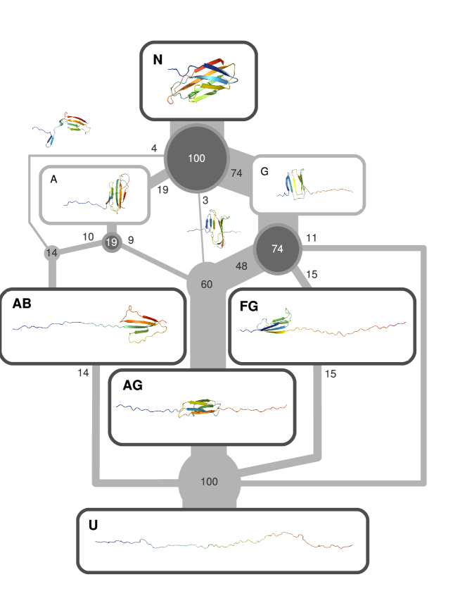
Figure 4: Illustration of the diversity of unfolding pathways in the 100 constant-velocity unfolding simulations at $v=0.03$ fm/MC step. The numbers indicate how many of the trajectories follow a certain path. The boxes illustrate important structures along the pathways and boxes with dark rims correspond to the most long-lived states. Dark circles mark branch points. Most trajectories pass through G or A, but only a fraction spend a significant amount of time there (see Table 4). The line directly from G to U corresponds to events that either have no intermediate at all or only have intermediates other than the main three. The direct lines N$\rightarrow$AB and N$\rightarrow$AG describe events that do not clearly pass through A or G and examples of structures seen in those events are illustrated by the unboxed cartoons next to the lines.

The unfolding pattern illustrated in Fig. 4 can be partly understood by counting native hydrogen bonds. The numbers of hydrogen bonds connecting the strand pairs AB, BE, CF and FG are $n_{\text{AB}}=7$, $n_{\text{BE}}=5$, $n_{\text{CF}}=8$ and $n_{\text{FG}}=6$, respectively. In our as well as in a previous study [17], two hydrogen bonds near the C terminus break early in some cases, which reduces the number of FG bonds to $n_{\text{FG}}=4$. The transition frequencies seen in Fig. 4 match well with the ordering $n_{\text{BE}}\sim n_{\text{FG}}<n_{\text{AB}}<n_{\text{CF}}$. The first branch point in Fig. 4 is the native state. Transitions from this state to the G state, N$\to$G, are more common than N$\to$A transitions, in line with the relation $n_{\text{FG}}<n_{\text{AB}}$. The second layer of branch points is the A and G states. That transitions G$\to$AG are more common than G$\to$GF and that A$\to$AG and A$\to$AB have similar frequencies, match well with the relations $n_{\text{AB}}<n_{\text{CF}}$ and $n_{\text{FG}}\sim n_{\text{BE}}$, respectively. Finally, there are fewer hydrogen bonds connecting the AB hairpin to the rest of the native structure than what is the case for the FG hairpin, $n_{\text{BE}}<n_{\text{CF}}$, which may explain why the AB hairpin, unlike the FG hairpin, detaches as one unit in some runs.

Another feature seen from Fig. 4 is that the remaining native-like core rotates during the course of the unfolding process. The orientation of the core is crucial, because a strand is much more easily released if it can be unzipped one hydrogen bond at a time, rather than by longitudinal pulling. The detachment of the first strand leads, irrespective of whether it is A or G, to an arrangement such that two strands are favorably positioned for unzipping, which explains why the intermediates with only A or G detached have a low force-resistance (see Tables 3 and 4). The AG, AB and FG intermediates, on the other hand, have cores that are pulled longitudinally, which makes them more resistant. Also worth noting is that the core of the AG intermediate is flipped 180^∘, which is not the case for the AB and FG intermediates.

The end-to-end distance of the intermediates cannot be directly compared with experimental data. The experiments measured  [12] contour-length differences rather than $L$, through worm-like chain (WLC) [45] fits to constant-velocity data. Using data at our lowest pulling velocity (0.03 fm/MC step), we now mimic this procedure. For each force peak, we determine a contour length $L_{\text{c}}$ by fitting the WLC expression

$$F=\frac{k_{\text{B}}T}{\xi}\left[\frac{1}{4(1-z/L_{\text{c}})^{2}}-\frac{1}{4}+\frac{z}{L_{\text{c}}}\right]$$ (7)

to data. Here $\xi$ denotes the persistence length and $z$ is the elongation, defined as $z=L-L_{\text{N}}$, where $L_{\text{N}}$ is the end-to-end distance of the native state. Following [12], we use a fixed persistence length of $\xi=0.4$ nm.

After each rupture peak follows a region where the force is relatively low. Here it sometimes happens that the newly released chain segment forms $\alpha$-helical structures, indicating that our system is not perfectly described by the simple WLC model. Nevertheless, the WLC model provides a quite good description of our unfolding traces, as illustrated by Fig. 5. The figure shows a typical unfolding trajectory with three force peaks, corresponding to the native (N), intermediate (I) and unfolded (U) states, respectively. From the fitted $L_{\text{c}}$ values, the contour-length differences $\Delta L_{\text{c}}(\text{N}\to\text{I})$, $\Delta L_{\text{c}}(\text{I}\to\text{U})$ and $\Delta L_{\text{c}}(\text{N}\to\text{U})$ can be calculated.

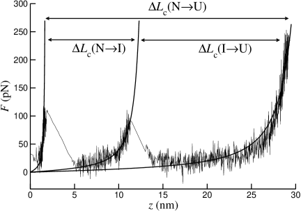
Figure 5: WLC fits (Eq. 7) to a typical force-extension curve at $v=0.03$ fm/MC step. The arrows indicate contour-length differences extracted from the fits: $\Delta L_{\text{c}}(\text{N}\to\text{I})$, $\Delta L_{\text{c}}(\text{I}\to\text{U})$ and $\Delta L_{\text{c}}(\text{N}\to\text{U})$.

Fig. 6 shows a histogram of $\Delta L_{\text{c}}(\text{N}\to\text{I})$, based on our 100 trajectories for $v=0.03$ fm/MC step. For a small fraction of the force peaks, a WLC fit is not possible; e.g., the A state cannot be analyzed due to its closeness to the native state. All intermediates analyzed have a $\Delta L_{\text{c}}(\text{N}\to\text{I})$ in the range 6–27 nm. They are divided into five groups: AB, AG, FG, G and “other”. Most of those in the category “other” have five strands detached (CDEFG or ABEFG) and a $\Delta L_{\text{c}}(\text{N}\to\text{I})$ larger than 21 nm. These intermediates were not identified in the experimental study [12], which did not report any $\Delta L_{\text{c}}(\text{N}\to\text{I})$ values larger than 18 nm. These high-$L$ intermediates mainly occur as a second intermediate, following one of the main intermediates, which perhaps explains why they were not observed in the experiments. The few remaining intermediates in the category “other” are all of the same kind, ABG, but show a large variation in $\Delta L_{\text{c}}(\text{N}\to\text{I})$, from 10 to 19 nm. The small values correspond to states where strand B actually is attached to the structured core, but through non-native hydrogen bonds.

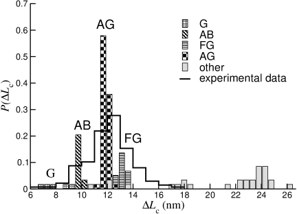
Figure 6: Histogram of the contour-length difference $\Delta L_{\text{c}}(\text{N}\to\text{I})$, obtained by WLC fits (Eq. 7) to our data for $v=0.03$ fm/MC step. A total of 121 force peaks corresponding to intermediate states are analyzed. The intermediates are divided into five groups: AB, AG, FG, G and “other”. The experimental $\Delta L_{\text{c}}(\text{N}\to\text{I})$ distribution, from [12], is also indicated.

The three major peaks in the $\Delta L_{\text{c}}(\text{N}\to\text{I})$ histogram (Fig. 6) correspond to the AG, AB and FG intermediates. Although similar in size, these states give rise to well separated peaks, the means of which differ in a statistically significant way (see Table 6). For comparison, Fig. 6 also shows the experimental $\Delta L_{\text{c}}(\text{N}\to\text{I})$ distribution  [12]. The statistical uncertainties appear to be larger in the experiments, because the distribution has a single broad peak extending from 6 to 18 nm. All our $\Delta L_{\text{c}}(\text{N}\to\text{I})$ data for the AB, AG, FG and G intermediates fall within this region. The occurrence of these four intermediates is thus consistent with the experimental $\Delta L_{\text{c}}(\text{N}\to\text{I})$ distribution. The highest peak, corresponding to the AG intermediate, is located near the center of the experimental distribution.

state	$\overline{\Delta L_{\text{c}}(\text{N}\to\text{I})}$ (nm)
AG	$12.1\pm 0.3$
AB	$10.1\pm 0.1$
FG	$13.4\pm 0.3$
G	$8.2\pm 0.9$

Table 6: The average contour-length difference $\overline{\Delta L_{\text{c}}(\text{N}\to\text{I})}$ for different intermediates, as obtained by WLC fits (Eq. 7) to our data for $v=0.03$ fm/MC step.

Transitions from the native state directly to the unfolded state do not occur in the trajectories analyzed for Fig. 6. For the contour-length difference between these two states, we find a value of $\Delta L_{\text{c}}(\text{N}\to\text{U})=30.9\pm 0.1$ nm, in perfect agreement with experimental data [12].

Estimating the free-energy profile

We now present the free-energy profile obtained by applying Eqs. 4–6 to the constant-velocity trajectories. The number of trajectories analyzed can be seen in Table 1. Fig. 7 shows the free-energy landscape at zero force, $G_{0}(L)$, against the end-to-end distance $L$, as obtained using different velocities $v$. We observe a collapse of the curves in the region of small-to-moderate $L$. Furthermore, the range of $L$ where the curves superimpose, expands as $v$ decreases. As discussed in [42, 28, 29, 30], the collapse of the reconstructed free-energy curves, as the manipulation rate is decreased, is a clear signature of the reliability of the evaluated free-energy landscape. Given our computational resources, we are not able to further decrease the velocity $v$, and for $L>15$ nm there is still a difference of $\sim$ 40 $k_{\text{B}}T$ between the two curves corresponding to the lowest velocities. The best estimate we currently have for $G_{0}(L)$ is the curve obtained with $v=0.03$ fm/MC step. This curve will be used in the following analysis.

Figure 7: Free-energy landscape $G_{0}(L)$ calculated as a function of the end-to-end distance $L$, using data at different pulling velocities $v$ (given in fm/MC step). In the calculations, $L$ is discretized with a bin size of $\Delta L=0.4$ nm for $v=1.0$ fm/MC step and $\Delta L=0.2$ nm for all the other velocities (see Model and Methods).

Let us consider the case where a constant force $F$ is applied to the chain ends. The free energy then becomes $G(L)=G_{0}(L)-F\cdot L$. The tilted free-energy landscape $G(L)$ is especially interesting for small forces for which the unfolding process is too slow to be studied through direct simulation.

Fig. 8 shows our calculated $G(L)$ for four external forces in the range 10–50 pN. At $F=10$ pN, the state with minimum free energy is still the native one, and no additional local minima have appeared. At $F=25$ pN, the situation has changed. For $20\lesssim F\lesssim 60$ pN, we find that $G(L)$ exhibits three major minima: the native minimum and two other minima, one of which corresponds to the fully unfolded state. The fully unfolded state takes over as the global minimum beyond $F=F_{\text{c}}\approx 22$ pN. The statistical uncertainty on the force at which this happens, $F_{\text{c}}$, is large, due to uncertainties on $G(L)$ for large $L$, as will be further discussed below. For $F=25$ pN, the positions of the three major minima are $4.3$ nm, 12 nm and 25 nm. As $F$ increases, the minima move slightly toward larger $L$; for $F=50$ pN, their positions are 4.6 nm, 14 nm and 29 nm. The first two minima become increasingly shallow with increasing $F$. For $F\gtrsim 60$ pN, the only surviving minimum is the third one, corresponding to the completely unfolded state.

Figure 8: Tilted free-energy landscape $G(L)=G_{0}(L)-F\cdot L$ for four different forces $F$. The unperturbed landscape $G_{0}(L)$ corresponds to the curve shown in Fig. 7 for $v=0.03$ fm/MC step. The minima of $G(L)$ are discussed in the text.

These results have to be compared with the analysis above, which showed that the system, on its way from the native to the fully unfolded state, often spends a significant amount of time in some partially unfolded intermediate state with $L$ around 12–16 nm. These intermediates should correspond to local free-energy minima along different unfolding pathways, but may or may not correspond to local minima of the global free energy $G(L)$, which is based on an average over the full conformational space. As we just saw, it turns out that $G(L)$ actually exhibits a minimum around 12–16 nm, where the most common intermediates are found. It is worth noting that above $\sim$ 25 pN this minimum gets weaker with increasing force. This trend is in agreement with the results shown in Table 2: the fraction of apparent two-state events, without any detectable intermediate, increases with increasing force.

For $F=25$ pN and $F=35$ pN, a fourth minimum can also be seen in Fig. 8, close to the native state. Its position is $\approx$ 6 nm. This minimum is weak and has already disappeared for $F=50$ pN. It corresponds to a state in which the two native $\beta$-sheets are slightly shifted relative to each other and aligned along the direction of the force, with all strands essentially intact. The appearance of this minimum is in good agreement with the results of Gao et al. [17]. In their unfolding trajectories, Gao et al. saw two early plateaus with small $L$, which in terms of our $G(L)$ should correspond to the native minimum and this $L\approx 6$ nm minimum. In our model, the $L\approx 6$ nm minimum represents a non-obligatory intermediate state; in many unfolding events, especially at high force, the molecule does not pass this state.

Finally, Fig. 9 illustrates a more detailed analysis of the native minimum of $G(L)$, for $20\,\text{pN}<F<60$ pN. In this force range, we find that the first barrier is always located at $L=5.0$ nm, whereas the position of the native minimum varies with force (see inset of Fig. 9). Hence, the distance between the native minimum and the barrier, $x_{\text{u}}$, depends on the applied force, as expected [46, 47, 48, 49]. Fig. 9 shows the force-dependence of the barrier height, $\Delta G(F)$. The solid line is a linear fit with slope $x_{\text{u}}=0.4$ nm, which describes the data quite well in the force range 25–56 pN. At lower force, the force-dependence is steeper; a linear fit to the data at low force gives a slope of $x_{\text{u}}=0.8$ nm (dashed line). Using this latter fit to extrapolate to zero force, we obtain a barrier estimate of $\Delta G(0)\approx 5$ kcal/mol. Due to the existence of the non-obligatory $L\approx 6$ nm intermediate, it is unclear how to relate this one-dimensional free-energy barrier to unfolding rates. Experimentally, barriers are indirectly probed, using unfolding kinetics. For FnIII₁₀, experiments found a zero-force barrier of 22.2 kcal/mol [11], using kinetics. For the unfolding length, an experimental value of $x_{\text{u}}=0.38$ nm was reported [11], based on data in the force range 50–115 pN. Our result $x_{\text{u}}=0.4$ nm obtained using the overlapping force range 25–56 pN, is in good agreement with this value.

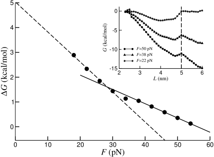
Figure 9: Free-energy barrier $\Delta G$, separating the native state from extended conformations, as a function of the pulling force $F$. The solid line is a linear fit to the data for forces $F>25$ pN, while the dashed line refers to a linear fit to the data in the interval $15\,\text{pN}\leq F\leq 30\,\text{pN}$. The inset shows the free energy $G(L)$ in the vicinity of the native state for three values of the force. The vertical dashed line indicates the position of the barrier.

Discussion

By AFM experiments, Li et al. [12] showed that FnIII₁₀ unfolds through intermediates when stretched by an external force. AFM data for the wild-type sequence and some engineered mutants were consistent with the existence of two distinct unfolding pathways with different intermediates, one being the AB state with strands A and B detached and the other being either the AG or the FG state [12]. This conclusion is in broad agreement with simulation results obtained by Paci and Karplus [15] and by Gao et al. [17].

Comparing our results with these previous simulations, one finds both differences and similarities. In our simulations, three major intermediates are observed: AB, which was seen by Paci and Karplus as well as by Gao et al.; AG, also seen by Paci and Karplus; and FG, which was not observed in previous studies. The most force-resistant intermediate is AB in our as well as in previous studies. Frequencies of occurrence of the intermediates are difficult to compare because the previous studies were based on fewer trajectories. Nevertheless, one may note that the most common intermediate in our simulations, AG, is one of two intermediates seen by Paci and Karplus, and corresponds to one of three pathways observed by Gao et al. A and G often being the first two strands to break is also in agreement with the simulation results of Klimov and Thirumalai [16], who studied several different proteins using a simplified model. Unlike us, these authors found a definite unfolding order for the $\beta$-strands. The first strand to break was G, followed by A.

A key issue in our study is how the unfolding pathway depends on the pulling strength. This question was addressed by Gao et al. [17]. Based on a simple analytical model rather than simulations, it was argued that there is a single unfolding pathway at low force and multiple unfolding pathways at high force. Our results show the opposite trend. At our lowest force, 50 pN, we observe several different unfolding pathways, and all the three major intermediates occur with a significant frequency. At our highest force, 192 pN, unfolding occurs either in one step or through one particular intermediate, the AG state. Moreover, at 192 pN, the same two strands, A and G, are almost always the first to break in the apparent one-step events as well. Hence, at our highest force, we find that the unfolding behavior has an essentially deterministic component. The trend that the unfolding pathway becomes more deterministic with increasing force can probably be attributed to a reduced relative importance of random thermal fluctuations.

There is a point of disagreement between our results and experimental data, which is that the rupture forces of the three major intermediates are higher in our constant-velocity simulations than they were in the experiments [12]. Although the statistical uncertainties are non-negligible and the pulling conditions are not identical (e.g., we consider a single FnIII₁₀ module, while the experiments studied multimodular constructs), we do not see any plausible explanation of this discrepancy. It thus seems that our model overestimates the rupture force of these intermediates. Our calculated rupture force for the native state is consistent with experimental data (see above). To make sure that this agreement is not accidental, we also measured the rupture force of the native state for three other domains, namely FnIII₁₂, FnIII₁₃ and the titin I27 domain. AFM experiments (at 0.6 $\mu$m/s) found that these domains differ in force-resistance, following the order FnIII₁₃ ($\sim$ 90 pN) $<$ FnIII₁₂ ($\sim$ 120 pN) $<$ I27 ($\sim$ 200 pN) [11]. For each of these domains, we carried out a set of 60 unfolding simulations, at a constant velocity of 0.10 fm/MC step. The average rupture forces were $108\pm 4$ pN for FnIII₁₃, $135\pm 4$ pN for FnIII₁₂, and $159\pm 6$ pN for I27, which is in reasonable agreement with experimental data. In particular, our model correctly predicts that the force-resistance of the native state decreases as follows: I27 $>$ FnIII₁₂$>$ FnIII₁₃$\sim$ FnIII₁₀. Similar findings have been reported for another model [18].

Throughout the paper, times have been given in MC steps. In order to roughly estimate what one MC step corresponds to in physical units, we use the average unfolding time of the native state, which is $\sim$ $4\cdot 10^{8}$ MC steps at our lowest force, 50 pN. Assuming that the force-dependence of the unfolding rate is given by $k(F)=k_{0}\exp(Fx_{\text{u}}/k_{\text{B}}T)$ [50] with $x_{\text{u}}=0.38$ nm [11], this unfolding time corresponds to a zero-force unfolding rate of $k_{0}\sim 1/(4\cdot 10^{10}\,\textrm{MC steps})$. Setting this quantity equal to its experimental value, $k_{0}=0.02\,\textrm{s}^{-1}$ [11], gives the relation that one MC step corresponds to $1\cdot 10^{-9}$ s. Using this relation to translate our pulling velocities into physical units, one finds, for example, that 0.05 fm/MC step corresponds to 0.05$\mu$m/s. This estimate suggests that the effective pulling velocities in our simulations are comparable to or lower than the typical pulling velocity in the experiments [12], which was $0.4\mu$m/s. That the effective pulling velocity is low in our simulations is supported by the observation made earlier that the force drops to very small values between the rupture peaks.

The force range studied in our simulations is comparable to that studied in AFM experiments [11, 12, 13]. The exact forces acting on fibronectin under physiological conditions are not known, but might be considerably smaller. For comparison, it was estimated that physiologically relevant forces for the muscle protein titin are $\sim$ 4 pN per I-band molecule [51]. For so small forces, the unfolding of FnIII₁₀ occurs too slowly in the model to permit direct simulation. Therefore, we cannot characterize unfolding pathways and possible intermediates for these forces. On the other hand, we have an estimate of the free-energy profile $G(L)$ for arbitrary force, which can be used, in particular, to estimate the force $F_{\text{c}}$, beyond which the fully extended state has minimum free energy. Using our best estimate of $G(L)$, one finds an $F_{\text{c}}$ of 22 pN (see above). Now, $F_{\text{c}}$ depends on the behavior of $G(L)$ for large $L$, where the uncertainties are large and not easy to accurately estimate. As a test, we therefore repeated the same analysis using the Ising-like model of [28, 29, 38] (unpublished results), which gave us the estimate $F_{\text{c}}\sim 20$ pN, in quite good agreement with the value found above (22 pN). Together, we take these results to indicate that $F_{\text{c}}\gtrsim 15$ pN, which might be large compared to physiologically relevant forces (see above). For stretching forces $F$ significantly smaller than $F_{\text{c}}$, the statistical weight of the fully stretched state is small. To estimate the suppression, let $L_{\text{N}}$ and $L_{\text{s}}$ be the end-to-end distances of the native and stretched states. The free energies of these states at force $F$ can be written as $G_{\text{N}}=G_{\text{N}}^{\text{c}}-(F-F_{\text{c}})L_{\text{N}}$ and $G_{\text{s}}=G_{\text{s}}^{\text{c}}-(F-F_{\text{c}})L_{\text{s}}$, where $G_{\text{N}}^{\text{c}}$ and $G_{\text{s}}^{\text{c}}$ are the free energies at $F_{\text{c}}$. Assuming $G_{\text{N}}^{\text{c}}=G_{\text{s}}^{\text{c}}$, $F_{\text{c}}\gtrsim 15$ pN and $L_{\text{s}}-L_{\text{N}}\sim 20$ nm, one finds, for example, that $G_{\text{s}}-G_{\text{N}}\gtrsim 25\,k_{\text{B}}T$ for $F\lesssim 10$ pN. Our estimate $F_{\text{c}}\gtrsim 15$ pN thus indicates that unfolding of FnIII₁₀ to its fully stretched state is a rare event for stretching forces $F\lesssim 10$ pN. The major intermediates are also suppressed compared to the native state for $F\lesssim 10$ pN (see Fig. 8). However, our results indicate that the major intermediates are more likely to be observed than the fully stretched state for these forces.

By extrapolating from experimental data at zero force, the force at which the native and fully stretched states have equal free energy has been estimated to be 3.5–5 pN for an average FnIII domain [52]. Our results suggest that the native state remains thermodynamically dominant at so small forces.

The reconstructed free energies $G_{0}(L)$ and $G(L)$ are thermodynamical potentials describing the equilibrium behavior of the system in the absence and presence of an external force $F$, respectively. On the other hand, the long-lived intermediate states observed during the unfolding of the molecule are a clear signature of out-of-equilibrium behavior. They indicate an arrest of the unfolding kinetics, typically in the $L$ range 12-16 nm, on the way from the old (native) equilibrium state to the new (fully unfolded) equilibrium state. The calculated (equilibrium) landscape $G(L)$ (see Fig. 8) is to some extent able to describe this out-of-equilibrium behavior. For $20\lesssim F\lesssim 60$ pN, this function exhibits three major minima corresponding to the folded state, the most common intermediates, and the fully unfolded state, respectively. However, since $G(L)$ describes the system in terms of a single coordinate $L$ and “hides” the microscopic configuration, one cannot extract the full details of individual unfolding pathways from this function. For example, one cannot, based on $G(L)$, distinguish the AG, AB and FG intermediates, which have quite similar $L$.

The height of the first free-energy barrier, $\Delta G$, can be related to the unfolding length $x_{\text{u}}$, a parameter typically extracted from unfolding kinetics, assuming the linear relationship $\Delta G(F)=\Delta G_{0}-F\cdot x_{\text{u}}$. The parameter $x_{\text{u}}$ measures the distance between the native state and the free-energy barrier, which generally depends on force. Our data for $x_{\text{u}}$ indeed show a clear force-dependence (see inset of Fig. 9). However, over a quite large force interval, our $x_{\text{u}}$ is almost constant and similar to its experimental value [12], which was based on an overlapping force interval.

Conclusion

We have used all-atom MC simulations to study the force-induced unfolding of the fibronectin module FnIII₁₀, and in particular how the unfolding pathway depends on the pulling conditions. Both at constant force and at constant pulling velocity, the same three major intermediates were seen, all with two native $\beta$-strands missing: AG, AB or FG. Contour-length differences $\Delta L_{\text{c}}(\text{N}\to\text{I})$ for these states were analyzed, through WLC fits to constant-velocity data. We found that the states, in principle, can be distinguished based on their $\Delta L_{\text{c}}(\text{N}\to\text{I})$ distributions, but the differences between the distributions are small compared to the resolution of existing experimental data.

The unfolding behavior at constant force was examined in the range 50–192 pN. The following picture emerges from this analysis:

1. At the lowest forces studied, several different unfolding pathways can be seen, and all the three major intermediates occur with a significant frequency.

2. At the highest forces studied, the AB and FG intermediates are very rare. Unfolding occurs either in an apparent single step or through the AG intermediate.

3. The unfolding behavior becomes more deterministic with increasing force. At 192 pN, the first strand pair to break is almost always A and G, also in apparent two-state events.

The dependence on pulling velocity in the constant-velocity simulations was found to be somewhat less pronounced, compared to the force-dependence in the constant-force simulations. Nevertheless, some clear trends could be seen in this case as well. In particular, with increasing velocity, we found that the AG state becomes increasingly dominant among the intermediates. Our results thus suggest that the AG state is the most important intermediate both at high constant force and at high constant velocity.

The response to weak pulling forces is expensive to simulate; our calculations, based on a relatively simple and computationally efficient model, extended down to 50 pN. The Jarzynski method for determining the free energy $G(L)$ opens up a possibility to partially circumvent this problem. Our estimated $G(L)$, which matches well with several direct observations from the simulations, indicates, in particular, that stretching forces below 10 pN only rarely unfold FnIII₁₀ to its fully extended state. Although supported by calculations based on a different model, this conclusion should be verified by further studies, because accurately determining $G(L)$ for large $L$ is a challenge.

Acknowledgments

This work has been in part supported by the Swedish Research Council and by the European Community via the STREP project EMBIO NEST (contract no. 12835).

References

- [1] Geiger, B., A. Bershadsky, R. Pankov, and K.M. Yamada. 2001. Transmembrane crosstalk between the extracellular matrix and the cytoskeleton. Nat. Rev. Mol. Cell Biol. 2:793–805.
- [2] Vogel, V. 2006. Mechanotransduction involving multimodular proteins: converting force into biochemical signals. Annu. Rev. Bioph. Biom. 35:459–488.
- [3] Ruoslahti, E., and M.D. Pierschbacher. 1987. New perspectives in cell adhesion: RGD and integrins. Science 238:491–497.
- [4] Aota, S.-I., M. Nomizu, and K.M. Yamada. 2004. The short amino acid sequence Pro-His-Ser-Arg-Asn in human fibronectin enhances cell-adhesive function. J. Biol. Chem. 269:24756–24761.
- [5] Krammer, A., H. Lu, B. Isralewitz, K. Schulten, and V. Vogel. 1999. Forced unfolding of the fibronectin type III module reveals a tensile molecular recognition switch. Proc. Natl. Acad. Sci. USA 96:1351–1356.
- [6] Ohashi, T., D.P. Kiehart, and H.P. Erickson. 1999. Dynamics and elasticity of the fibronectin matrix in living cell culture visualized by fibronectin-green fluorescent protein. Proc. Natl. Acad. Sci. USA 96:2153–2158.
- [7] Abu-Lail, N.I., T. Ohashi, R.L. Clark, H.P. Erickson, S. Zauscher. 2006. Understanding the elasticity of fibronectin fibrils: unfolding strengths of FN-III and GFP domains measured by single molecule force spectroscopy. Matrix Biol. 25:175–184.
- [8] Baneyx, G., L. Baugh, and V. Vogel. 2002. Fibronectin extension and unfolding within cell matrix fibrils controlled by cytoskeletal tension Proc. Natl. Acad. Sci. USA 99:5139–5143.
- [9] Smith, M.L.,D. Gourdon, W.C. Little, K.E. Kubow, R. Andresen Eguiluz, S. Luna-Morris, and V. Vogel. 2007. Force-induced unfolding of fibronectin in the extracellular matrix of living cells. PLoS Biol. 5:e268.
- [10] Plaxco, K.W., C. Spitzfaden, I.D. Campbell, and C.M. Dobson. 1997. A comparison of the folding kinetics and thermodynamics of two homologous fibronection type III modules. J. Mol. Biol. 270:763–770.
- [11] Oberhauser, A.F., C. Badilla-Fernandez, M. Carrion-Vazquez, and J.M. Fernandez. 2002. The mechanical hierarchies of fibronectin observed by single-molecule AFM. J. Mol. Biol. 319:433–447.
- [12] Li, L., H.H.-L. Huang, C.L. Badilla, and J.M. Fernandez. 2005. Mechanical unfolding intermediates observed by single-molecule force spectroscopy in a fibronectin type III module. J. Mol. Biol. 345:817–826.
- [13] Ng, S.P., and J. Clarke. 2007. Experiments suggest that simulations may overestimate electrostatic contributions to the mechanical stability of a fibronectin type III domain. J. Mol. Biol. 371:851–854.
- [14] Cota, E., and J. Clarke. 2000. Folding of beta-sandwich proteins: three-state transition of a fibronectin type III module. Protein Sci. 9:112–120.
- [15] Paci, E., and M. Karplus. 1999. Forced unfolding of fibronectin type 3 modules: an analysis by biased molecular dynamics simulations. J. Mol. Biol. 288:441–459.
- [16] Klimov, D.K., and D. Thirumalai. 2000. Native topology determines force-induced unfolding pathways in globular proteins. Proc. Natl. Acad. Sci. USA 97:7254–7259.
- [17] Gao, M., D. Craig, V. Vogel, and K. Schulten. 2002. Identifying unfolding intermediates of FnIII10 by steered molecular dynamics. J. Mol. Biol. 323:939–950.
- [18] Craig, D., M. Gao, K. Schulten, and V. Vogel. 2004. Tuning the mechanical stability of fibronectin type III modules through sequence variations. Structure 12:21–30.
- [19] Sułkowska, J.I., and M. Cieplak. 2007. Mechanical stretching of proteins — a theoretical survey of the Protein Data Bank. J. Phys.: Condens. Matter 19:283201.
- [20] Li, M.S. 2007. Secondary structure, mechanical stability, and location of transition state of proteins. Biophys. J. 93:2644–2654.
- [21] Irbäck, A., B. Samuelsson, F. Sjunnesson, and S. Wallin. 2003. Thermodynamics of - and -structure formation in proteins. Biophys. J. 85:1466–1473.
- [22] Irbäck, A., and S. Mohanty. 2005. Folding thermodynamics of peptides. Biophys. J. 88: 1560–1569.
- [23] Lu, H., and K. Schulten. 2000. The key event in force-induced unfolding of titin’s immunoglobulin domains. Biophys. J. 79: 51–65.
- [24] Jarzynski, C. 1997. Nonequilibrium equality for free energy differences. Phys. Rev. Lett. 78:2690–2693.
- [25] Crooks, G.E. 1999. Energy production fluctuation theorem and the nonequilibrium work relation for free energy differences. Phys. Rev. E 60:2721–2726.
- [26] Hummer, G., and A. Szabo. 2001. Free energy reconstruction from nonequilibrium single-molecule pulling experiments. Proc. Natl. Acad. Sci. USA 98:3658–3661.
- [27] West, D.K., P.D. Olmsted, and E. Paci. 2006. Free energy for protein folding from nonequilibrium simulations using the Jarzynski equality. J. Chem. Phys. 125:204910.
- [28] Imparato, A., A. Pelizzola, and M. Zamparo. 2007. Ising-like model for protein mechanical unfolding. Phys. Rev. Lett. 98:148102.
- [29] Imparato, A., A. Pelizzola, and M. Zamparo. 2007. Protein mechanical unfolding: a model with binary variables. J. Chem. Phys. 127:145105.
- [30] Imparato, A., S. Luccioli, and A. Torcini. 2007. Reconstructing the free-energy landscape of a mechanically unfolded model protein. Phys. Rev. Lett. 99:168101.
- [31] Harris, N.C., Y. Song, and C.-H. Kiang. 2007. Experimental free energy surface reconstruction from single-molecule force spectroscopy using Jarzynski’s equality. Phys. Rev. Lett. 99: 068101.
- [32] Imparato, A., F. Sbrana, and M. Vassalli. 2008. Reconstructing the free-energy landscape of a polyprotein by single-molecule experiments. EPL 82:58006.
- [33] Irbäck, A., S. Mitternacht, and S. Mohanty. 2005. Dissecting the mechanical unfolding of ubiquitin. Proc. Natl. Acad. Sci. USA 102:13427–13432.
- [34] Irbäck, A., and S. Mitternacht. 2006. Thermal versus mechanical unfolding of ubiquitin. Proteins 65:759–766.
- [35] Schlierf, M., H. Li, and J.M. Fernandez. 2004. The unfolding kinetics of ubiquitin captured with single-molecule force-clamp techniques. Proc. Natl. Acad. Sci. USA 101:7299–7304.
- [36] Li, M.S., M. Kouza, and C.K. Hu. 2007. Refolding upon force quench and pathways of mechaincal and thermal unfolding of ubiquitin. Biophys. J. 92:547–561.
- [37] Kleiner, A., and E. Shakhnovich. 2007. The mechanical unfolding of ubiquitin through all-atom Monte Carlo simulation with a Gō-type potential. Biophys. J. 92:2054–2061.
- [38] Imparato, A., and A. Pelizzola. 2008. Mechanical unfolding and refolding pathways of ubiquitin. 2008. Phys. Rev. Lett. 100:158104.
- [39] Favrin, G., A. Irbäck, and F. Sjunnesson. 2001. Monte Carlo update for chain molecules: biased Gaussian steps in torsional space. J. Chem. Phys. 114: 8154–8158.
- [40] Irbäck, A., and S. Mohanty. 2006. PROFASI: a Monte Carlo simulation package for protein folding and aggregation. J. Comput. Chem. 27: 1548–1555.
- [41] DeLano, W.L. 2002. The PyMOL molecular graphics system. San Carlos, CA: DeLano Scientific.
- [42] Imparato A., and L. Peliti. 2006. Evaluation of free energy landscapes from manipulation experiments. J. Stat. Mech. P03005.
- [43] Ferrenberg A.M., and R. H. Swendsen. 1989. Optimized Monte Carlo analysis. Phys. Rev. Lett. 63: 1195–1198.
- [44] Evans, E., and K. Ritchie. 1997. Dynamic strength of molecular adhesion bonds. Biophys. J. 72: 1541–1555.
- [45] Marko, J.F., and E.D. Siggia. 1995. Stretching DNA. Macromolecules 28:8759–8770.
- [46] Li, P.-C., and D.E. Makarov. 2003. Theoretical studies of the mechanical unfolding of the muscle protein titin: bridging the time-scale gap between simulation and experiment. J. Chem. Phys. 119:9260–9268.
- [47] Hyeon, C., and D. Thirumalai. 2006. Forced-unfolding and force-quench refolding of RNA hairpins. Biophys. J. 90:3410–3427.
- [48] West, D.K., E. Paci, and P.D. Olmsted. 2006. Internal protein dynamics shifts the distance to the mechanical transition state. Phys. Rev. E 74:061912.
- [49] Dudko, O.K., J. Mathé, A. Szabo, A. Meller, and G. Hummer. 2007. Extracting kinetics from single-molecule force spectroscopy: nanopore unzipping of DNA hairpins. Biophys. J. 92:4186–4195.
- [50] Bell, G.I. 1978. Models for specific adhesion of cells to cells. Science 200:618–627.
- [51] Li, H., W.A. Linke, A.F. Oberhauser, M. Carrion-Vazquez, J.G. Kerkvliet, H. Lu, P.E. Marszalek, and J.M. Fernandez. 2002. Reverse engineering of the giant muscle protein titin. Nature 418:998–1002.
- [52] Erickson, H.P. 1994. Reversible unfolding of fibronectin type III and immunoglobulin domains provides the structural basis for stretch and elasticity of titin and fibronectin. Proc. Natl. Acad. Sci. USA 91:10114–10118.
- [53] Main, A.L., T.S. Harvey, M. Baron, J. Boyd, and I.D. Campbell. 1992. The three-dimensional structure of the tenth type III module of fibronectin: an insight into RGD-mediated interactions. Cell 71:671–678.