Diversity Analysis of Bit-Interleaved Coded Multiple Beamforming

Abstract

In this paper, diversity analysis of bit-interleaved coded multiple beamforming (BICMB) is extended to the case of general spatial interleavers, removing a condition on their previously known design criteria and quantifying the resulting diversity order. The diversity order is determined by a parameter $Q_{max}$ which is inherited from the convolutional code and the spatial de-multiplexer used in BICMB. We introduce a method to find this parameter by employing a transfer function approach as in finding the weight spectrum of a convolutional code. By using this method, several $Q_{max}$ values are shown and verified to be identical with the results from a computer search. The diversity analysis and the method to find the parameter are supported by simulation results. By using the Singleton bound, we also show that $Q_{max}$ is lower bounded by the product of the number of streams and the code rate of an encoder. The design rule of the spatial de-multiplexer for a given convolutional code is proposed to meet the condition on the maximum achievable diversity order.

I Introduction

When the channel information is perfectly available at the transmitter, beamforming is an attractive technique to enhance the performance of a multi-input multi-output (MIMO) system [1]. A set of beamforming vectors is obtained by singular value decomposition (SVD) which is optimal in terms of minimizing the average bit error rate (BER) [2]. Single beamforming, which carries only one symbol at a time, was shown to achieve full diversity order of $NM$ where $N$ is the number of transmit antennas and $M$ is the number of receive antennas [3], [4]. However, multiple beamforming, which increases the throughput by sending multiple symbols at a time, loses the full diversity order over flat fading channels.

To achieve the full diversity order as well as the full spatial multiplexing order, bit-interleaved coded multiple beamforming, combining bit-interleaved coded modulation (BICM) and multiple beamforming, was introduced in [5]. Design criteria for interleaving the coded sequence were provided such that each subchannel created by SVD is utilized at least once with a corresponding channel bit equal to $1$ in an error event on the trellis diagram [5], [6]. BICMB with $1/2$-rate convolutional encoder, a simple interleaver and soft-input Viterbi decoder was shown to have full diversity order when it is used in a $2\times 2$ system with $2$ streams. In this paper, the diversity order is analyzed even when the interleaver does not meet the criteria of [5], [6]. To determine the diversity order, the error events that dominate BER performance need to be found. We introduce a method to find the dominant error events by extending a method from convolutional code analysis to determine system performance, e.g., [7], [8], into the analysis of the given combination of the interleaver and the code. We also show that for any convolutional code and any spatial de-multiplexer, the maximum achievable diversity order is related with the product of the code rate and the number of streams, by using the Singleton bound [9]. The design rule of the spatial de-multiplexer to get the maximum achievable diversity order is also proposed.

The rest of this paper is organized as follows. A brief review of the BICMB system is given in Section II. Section III introduces a method to find $\alpha$-vectors for a given convolutional code and the number of subchannels. Pairwise error probability (PEP) analysis is given in Section IV. In Section V, the analysis of the maximum achievable diversity order of BICMB is shown, and the design rule of the spatial de-multiplexer for the maximum achievable diversity order is proposed. Simulation results supporting the analysis are shown in Section VI. Finally, we end the paper with a conclusion in VII.

II BICMB Overview

The code rate $R_{c}=k_{c}/n_{c}$ convolutional encoder, possibly combined with a perforation matrix for a high rate punctured code, generates the codeword $\mathbf{c}$ from the information vector $\mathbf{b}$. Then, the spatial de-multiplexer distributes the coded bits into $S$ sequences, each of which is interleaved by an independent bit-wise interleaver. The interleaved sequences $\mathbf{D}$ are mapped by Gray encoding onto the symbol sequences $\mathbf{Y}$. A symbol belongs to a signal set $\chi\subset\mathbb{C}$ of size $|\chi|=2^{m}$, such as $2^{m}$-QAM, where $m$ is the number of input bits to the Gray encoder.

The MIMO channel $\mathbf{H}\in\mathbb{C}^{M\times N}$ is assumed to be quasi-static, Rayleigh, and flat fading, and perfectly known to both the transmitter and the receiver. In this channel model, we assume that the channel coefficients remain constant for the $L$ symbol duration. The beamforming vectors are determined by the singular value decomposition of the MIMO channel, i.e., $\mathbf{H}=\mathbf{U\Lambda V^{H}}$ where $\mathbf{U}$ and $\mathbf{V}$ are unitary matrices, and $\mathbf{\Lambda}$ is a diagonal matrix whose $s^{th}$ diagonal element, $\lambda_{s}\in\mathbb{R}$, is a singular value of $\mathbf{H}$ with decreasing order. When $S$ symbols are transmitted at the same time, then the first $S$ vectors of $\mathbf{U}$ and $\mathbf{V}$ are chosen to be used as beamforming matrices at the receiver and the transmitter, respectively. Let’s denote the first $S$ vectors of $\mathbf{U}$ and $\mathbf{V}$ as $\mathbf{\tilde{U}}$ and $\mathbf{\tilde{V}}$. The system input-output relation at the $k^{th}$ time instant for a packet duration is written as

$$\mathbf{r}_{k}=\mathbf{\tilde{U}}^{H}\mathbf{H}\mathbf{\tilde{V}}\mathbf{y}_{k}+\mathbf{\tilde{U}}^{H}\mathbf{n}_{k}$$ (1)

where $\mathbf{y}_{k}$ is an $S\times 1$ vector of transmitted symbols, $\mathbf{r}_{k}$ is an $S\times 1$ vector of the detected symbols, and $\mathbf{n}_{k}$ is an additive white Gaussian noise vector with zero mean and variance $N_{0}=N/SNR$. On each $s^{th}$ subchannel, finally, we get

$$r_{k,s}=\lambda_{s}y_{k,s}+\tilde{n}_{k,s}$$ (2)

where $r_{k,s}$, $y_{k,s}$, and $\tilde{n}_{k,s}$ are a detected symbol, a transmitted symbol, and a noise term, respectively. $\mathbf{H}$ is complex Gaussian with zero mean and unit variance, and to make the received signal-to-noise ratio $SNR$, the total transmitted power is scaled as $N$. The equivalent system model is shown in Fig. 1.

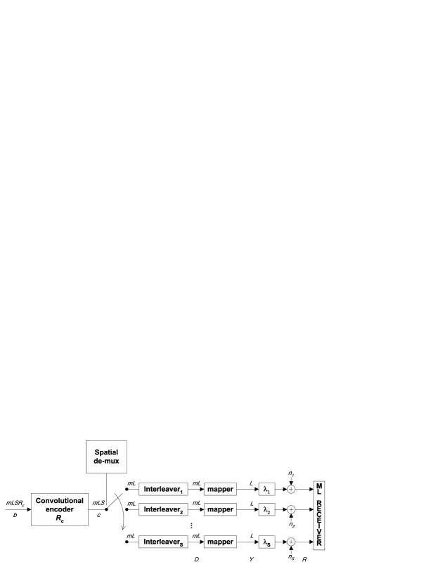
Figure 1: Equivalent system model of BICMB

The location of the $l^{th}$ coded bit $c_{l}$ within the detected symbols is stored in a table $l\rightarrow(k,s,i)$, where $k$, $s$, and $i$ are time instant, subchannel, and bit position on a symbol, respectively. Let $\chi_{b}^{i}\subset\chi$ where $b\in\{0,1\}$ in the $i^{th}$ bit position. By using the information in the table and the input-output relation in (2), the receiver calculates the ML bit metrics as

$$\gamma^{i}(r_{k,s},c_{l})=\min_{y\in\chi_{c_{l}}^{i}}|r_{k,s}-\lambda_{s}y|^{2}.$$ (3)

The combination of the ML bit metrics of (3) and $\mathbf{\tilde{U}}$ detector at the receiver is not the unique solution to get the optimum BER performance. Appropriate bit metrics corresponding to a linear detector, such as zero-forcing (ZF) or minimum mean square error (MMSE) detector, were shown to be equivalent to the bit metrics of (3) with $\mathbf{\tilde{U}}$ detector [10]. Finally, the ML decoder can make decisions according to the rule

$$\mathbf{\hat{c}}=\arg\min_{\mathbf{\tilde{c}}}\sum_{l}\gamma^{i}(r_{k,s},\tilde{c}_{l}).$$ (4)

III $\alpha$-Spectra

The BER of a BICMB system is upper bounded by all the summations of each pairwise error probability for all the error events on the trellis [5], [6]. Therefore, the calculation of PEP for each error event is needed to analyze the diversity order of a given BICMB system. If the interleaver is properly designed such that the consecutive long coded bits are mapped onto distinct symbols, the PEP between the two codewords $\mathbf{c}$ and $\mathbf{\hat{c}}$ with Hamming distance $d_{H}$ is upper bounded as [5]

$$P\left(\mathbf{c}\rightarrow\mathbf{\hat{c}}\right) =E\left[P\left(\mathbf{c}\rightarrow\mathbf{\hat{c}}|\mathbf{H}\right)\right]$$

$$\leq E\left[\frac{1}{2}\exp\left(-\frac{d^{2}_{min}\sum\limits_{s=1}^{S}\alpha_{s}\lambda_{s}^{2}}{4N_{0}}\right)\right]$$ (5)

where $d_{min}$ is the minimum Euclidean distance in the constellation and $\alpha_{s}$ denotes the number of times the $s^{th}$ subchannel is used corresponding to $d_{H}$ bits under consideration, satisfying $\sum_{s=1}^{S}\alpha_{s}=d_{H}$. Since PEP is affected by the summation of the products between $\alpha_{s}$ and singular values as can be seen in (5), it is important to calculate the $\alpha$-vectors for each error path to have an insight into the diversity order behavior of a particular BICMB implementation.

It has been shown in [5], [6] that for a single-carrier BICMB system, if the interleaver is designed such that, for all error paths of interest with Hamming distance $d_{H}$ to the all-zeros path,

1. the consecutive coded bits are mapped over different symbols,

2. $\alpha_{s}\geq 1$ for $1\leq s\leq S$,

then the BICMB system achieves full diversity. In this paper, we will analyze cases where the sufficient condition $\alpha_{s}\geq 1$ may not be satisfied, i.e., $\alpha_{s}=0$ for some $s=1,2,\cdots,S$ is possible. In order to carry out this analysis, as well as to get an insight into the system behavior in [5], [6], one needs a method to calculate the values of $\alpha_{s}$ (which we call the $\alpha$-vector) of an error path at Hamming distance $d_{H}$ to the all-zeros path.

We developed a method to calculate the $\alpha$-vectors for a convolutional code and interleaver combination. We will now illustrate this method with a simple example. For this example, the system is composed of a $4$-state $1/2$-rate convolutional encoder and a spatial de-multiplexer rotating with an order of $a$, $b$, $c$, and $d$ which represent the four streams of transmission. Fig. 2 represents a trellis diagram of this convolutional encoder for one period at the steady state. Since a convolutional code is linear, the all-zero codeword is assumed to be the input to the encoder. To find a transfer function of a convolutional code and a spatial de-multiplexer, we label the branches as a combination of $a^{\phi_{a}}$, $b^{\phi_{b}}$, $c^{\phi_{c}}$, and $d^{\phi_{d}}$, where the exponent $\phi_{i}$ denotes the number of usage of the subchannel $i$ which contributes to detecting the wrong branch by the detector. Additionally, $Z^{\phi_{Z}}$, whose exponent satisfies $\phi_{Z}=\phi_{a}+\phi_{b}+\phi_{c}+\phi_{d}$, is included to get the relationship between the Hamming distance $d_{H}$ and $\alpha$-vector of an error event. Furthermore, the non-zero states are arbitrarily labeled $X_{11}$ through $X_{23}$, while the zero state is labeled as $X_{i}$ if branches split and $X_{o}$ if branches merge as shown in Fig. 2.

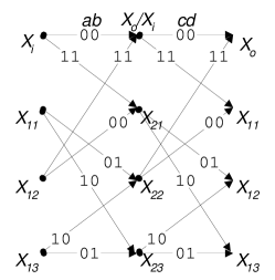
Figure 2: Trellis of $4$-state $1/2$-rate convolutional code with $4$ streams

Let’s denote $\mathbf{x}$ = $\left[\begin{array}[]{cccccc}X_{11}&X_{12}&X_{13}&X_{21}&X_{22}&X_{23}\end{array}\right]^{T}$. Then, the state equations are given by the matrix equation

$$\mathbf{x} =\mathbf{Fx}+\mathbf{t}X_{i}=\left[\begin{array}[]{cccccc}0&0&0&0&1&0\\ 0&0&0&dZ&0&cZ\\ 0&0&0&cZ&0&dZ\\ 0&1&0&0&0&0\\ bZ&0&aZ&0&0&0\\ aZ&0&bZ&0&0&0\end{array}\right]\mathbf{x}+\left[\begin{array}[]{c}cdZ^{2}\\ 0\\ 0\\ abZ^{2}\\ 0\\ 0\end{array}\right]X_{i}.$$ (18)

We also get

$$X_{o}=\mathbf{gx}=\left[\begin{array}[]{cccccc}0&abZ^{2}&0&0&cdZ^{2}&0\end{array}\right]\mathbf{x}.$$ (20)

The transfer function is represented in closed form by using the method in [8] as

$$\mathbf{T}(a,b,c,d,Z) =\mathbf{g}\left[\mathbf{I}-\mathbf{F}\right]^{-1}\mathbf{t}=\mathbf{gt}+\sum\limits_{k=1}^{\infty}\mathbf{gF}^{k}\mathbf{t}$$

$$=Z^{5}(a^{2}b^{2}d+bc^{2}d^{2})$$

$$+Z^{6}(2a^{2}bc^{2}d+a^{2}b^{2}d^{2}+b^{2}c^{2}d^{2})$$

$$+Z^{7}(a^{2}b^{3}c^{2}+2a^{2}b^{2}c^{2}d+2a^{2}bc^{2}d^{2}+$$ (21)

$$\quad\qquad b^{3}c^{2}d^{2}+a^{2}b^{2}d^{3}+a^{2}c^{2}d^{3})$$

$$+Z^{8}(a^{4}b^{2}c^{2}+4a^{2}b^{3}c^{2}d+4a^{2}b^{2}c^{2}d^{2}+$$

$$\quad\qquad b^{4}c^{2}d^{2}+a^{2}c^{4}d^{2}+4a^{2}bc^{2}d^{3}+a^{2}b^{2}d^{4})+\cdots$$

where $[\mathbf{I}-\mathbf{F}]^{-1}$ can be expanded as $\mathbf{I}+\mathbf{F}+\mathbf{F}^{2}+\cdots$ through an infinite series of power of matrices. The weight spectrum, used for error performance analysis of convolutional codes, can be easily determined by $\mathbf{T}(a,b,c,d,Z)\mid_{a=b=c=d=1}$ and can be compared with the literature [11], [12].

Assume that $a$, $b$, $c$, $d$ are assigned to be the stream numbers $1$, $2$, $3$, and $4$, respectively. We can then figure out from the transfer function that the $\alpha$-vectors of two error events with Hamming distance equal to $5$ are $[2\,2\,0\,1]$ and $[0\,1\,2\,2]$. Besides, the vectors with $\alpha_{1}$ equal to $0$ are easily found by choosing the terms composed of only $b$, $c$, and $d$, which are $[0\,1\,2\,2]$, $[0\,2\,2\,2]$, $[0\,3\,2\,2]$, and $[0\,4\,2\,2]$. No vector is found which has $\alpha_{1}$ = $\alpha_{2}$ = 0 or $\alpha_{1}$ = $\alpha_{2}$ = $\alpha_{3}$ = 0.

This method can be applied to any $\mathcal{K}$-state $k_{c}/n_{c}$-rate convolutional code and $S$-stream BICMB system. If the spatial de-multiplexer is not a random switch for the whole packet, the period of the spatial de-multiplexer is an integer multiple of the least common multiple (LCM) of $n_{c}$ and $S$. Note that we restrict a period of the interleaver to correspond to an integer multiple of trellis sections. Let’s denote $P$ = $LCM(n_{c},S)$ which means the number of coded bits for a minimum period. Then, the dimension of the vector $\mathbf{x}$ is $nP(\mathcal{K}-1)k_{c}/n_{c}$ where $n$ is the integer multiple for a period of interest.

By using this method, transfer functions of a $4$-state $1/2$-rate convolutional code with generator polynomials $(5,7)$ in octal combined with several different de-multiplexers are shown in (III), (III), and (III). The spatial de-multiplexer used in $\mathbf{T}_{1}$ and $\mathbf{T}_{2}$ is a simple rotating switch on $2$ and $3$ subchannels, respectively. For $\mathbf{T}_{3}$, $i^{th}$ coded bit is de-multiplexed into subchannel $s_{\mathrm{mod}(i,18)+1}$ where $s_{1}$ = $\cdots$ = $s_{6}$ = $1$, $s_{7}$ = $\cdots$ = $s_{12}$ = $2$, $s_{13}$ = $\cdots$ = $s_{18}$ = $3$ and $\mathrm{mod}$ is the modulo operation. Throughout the transfer functions, the variables $a$, $b$, and $c$ represent $1^{st}$, $2^{nd}$, and $3^{rd}$ subchannel, respectively, in a decreasing order of singular values from the channel matrix.

$$\mathbf{T}_{1} =Z^{5}(a^{2}b^{3})+Z^{6}(a^{4}b^{2}+a^{2}b^{4})$$

$$+Z^{7}(3a^{4}b^{3}+a^{2}b^{5})$$

$$+Z^{8}(a^{6}b^{2}+6a^{4}b^{4}+a^{2}b^{6})$$ (22)

$$+Z^{9}(5a^{6}b^{3}+10a^{4}b^{5}+a^{2}b^{7})$$

$$+Z^{10}(a^{8}b^{2}+15a^{6}b^{4}+15a^{4}b^{6}+a^{2}b^{8})+\cdots$$

$$\mathbf{T}_{2} =Z^{5}(a^{2}b^{2}c+a^{2}bc^{2}+ab^{2}c^{2})$$

$$+Z^{6}(a^{3}b^{2}c+a^{2}b^{3}c+a^{3}bc^{2}+$$

$$\quad\qquad ab^{3}c^{2}+a^{2}bc^{3}+ab^{2}c^{3})$$

$$+Z^{7}(2a^{3}b^{3}c+2a^{3}b^{2}c^{2}+2a^{2}b^{3}c^{2}+$$

$$\quad\qquad 2a^{3}bc^{3}+2a^{2}b^{2}c^{3}+2ab^{3}c^{3})$$ (23)

$$+Z^{8}(a^{5}b^{3}+a^{4}b^{3}c+a^{3}b^{4}c+2a^{4}b^{2}c^{2}+$$

$$\quad\qquad 3a^{3}b^{3}c^{2}+2a^{2}b^{4}c^{2}+a^{4}bc^{3}+3a^{3}b^{2}c^{3}+$$

$$\quad\qquad 3a^{2}b^{3}c^{3}+ab^{4}c^{3}+b^{5}c^{3}+a^{3}bc^{4}+$$

$$\quad\qquad 2a^{2}b^{2}c^{4}+ab^{3}c^{4}+a^{3}c^{5})+\cdots$$

$$\mathbf{T}_{3} =Z^{5}(a^{5}+a^{3}b^{2}+a^{2}b^{3}+$$

$$\quad\qquad b^{5}+a^{3}c^{2}+b^{3}c^{2}+a^{2}c^{3}+b^{2}c^{3}+c^{5})$$

$$+Z^{6}(a^{4}b^{2}+3a^{3}b^{3}+a^{2}b^{4}+a^{4}c^{2}+3a^{2}b^{2}c^{2}+$$

$$\quad\qquad b^{4}c^{2}+3a^{3}c^{3}+3b^{3}c^{3}+a^{2}c^{4}+b^{2}c^{4})$$ (24)

$$+Z^{7}(2a^{4}b^{3}+2a^{3}b^{4}+a^{3}b^{3}c+7a^{3}b^{2}c^{2}+$$

$$\quad\qquad 7a^{2}b^{3}c^{2}+2a^{4}c^{3}+a^{3}bc^{3}+7a^{2}b^{2}c^{3}+$$

$$\quad\qquad ab^{3}c^{3}+2b^{4}c^{3}+2a^{3}c^{4}+2b^{3}c^{4})+\cdots$$

$\mathbf{T}_{1}$ shows no term that lacks any of variables $a$ and $b$, which means the interleaver satisfies the full diversity order criterion, $\alpha_{s}\geq 1$ for $s$ = $1$, $2$ [5], [6]. Most of the terms in $\mathbf{T}_{2}$ are comprised of three variables, $a$, $b$, and $c$. However, three error events with Hamming distance of $8$ lack one variable, resulting in the $\alpha$-vectors as $[5\,3\,0]$, $[0\,5\,3]$, and $[3\,0\,5]$. In $\mathbf{T}_{3}$, many terms missing one or two variables are observed. Especially, vectors with $\alpha_{s}=0$ for two subchannels can be found as $[5\,0\,0]$, $[0\,5\,0]$, and $[0\,0\,5]$. In Section IV, we present how these vectors affect the diversity order of BICMB.

IV Diversity Analysis

Through the transfer functions in Section III, we have seen interleavers which do not guarantee the full diversity criteria. As stated previously, contrary to the assumption in [5] that $\alpha_{s}\geq 1$ for $s=1,2,\cdots,S$, we assume in this paper that it is possible to have $\alpha_{s}=0$ for some $s=1,2,\cdots,S$. Let’s define $\alpha_{nzmin}$ as the minimum $\alpha$ among the nonzero $\alpha$’s in the $\alpha$-vector. Using the inequality $\sum_{s=1}^{S}\alpha_{s}\lambda_{s}^{2}\geq\alpha_{nzmin}\sum_{k=1,\alpha_{k}\neq 0}^{S}\lambda_{k}^{2}$, PEP in (5) can be expressed as

$$P\left(\mathbf{c}\rightarrow\mathbf{\hat{c}}\right)\leq E\left[\frac{1}{2}\exp\left(-W\sum\limits_{k=1}^{K}\mu_{\ell{(k)}}\right)\right]$$ (25)

where $W=d^{2}_{min}\alpha_{nzmin}/(4N_{0})$, $K$ is the number of nonzero $\alpha$’s, $\ell(k)$ is an index to indicate the $k^{th}$ nonzero $\alpha$, and $\mu_{s}=\lambda_{s}^{2}$. To solve (25), we need the marginal pdf $f\left(\mu_{\ell(1)},\cdots,\mu_{\ell(K)}\right)$ by calculating

$$f\left(\mu_{\ell(1)},\cdots,\mu_{\ell(K)}\right)=\int_{0}^{\infty}\int_{0}^{\mu_{1}}\cdots\int_{0}^{\mu_{\ell(1)-2}}\int_{0}^{\mu_{\ell(1)}}\cdots\int_{0}^{\mu_{N-1}}\rho\left(\mu_{1},\cdots,\mu_{N}\right)\\ \times d_{\mu_{N}}\cdots d_{\mu_{\ell(1)+1}}d_{\mu_{\ell(1)-1}}\cdots d_{\mu_{2}}d_{\mu_{1}}.$$ (26)

The joint pdf $\rho\left(\mu_{1},\cdots,\mu_{N}\right)$ in (26) is available in the literature [13], [14] as

$$\rho\left(\mu_{1},\cdots,\mu_{N}\right)=p\left(\mu_{1},\cdots,\mu_{N}\right)e^{-\sum\limits_{i=1}^{N}\mu_{i}}$$ (27)

where the polynomial $p\left(\mu_{1},\cdots,\mu_{N}\right)$ is

$$p\left(\mu_{1},\cdots,\mu_{N}\right)=\prod^{N}_{i=1}\mu_{i}^{M-N}\prod^{N}_{j>i}\left(\mu_{i}-\mu_{j}\right)^{2}.$$ (28)

Because we are interested in the exponent of $W$, the constant, which appears in the literature, is ignored in (28) for brevity.

Let’s introduce $\hat{f}\left(\mu_{\ell(1)},\cdots,\mu_{\ell(K)}\right)$ which is defined as

$$\hat{f}\left(\mu_{\ell(1)},\cdots,\mu_{\ell(K)}\right)=\int_{0}^{\infty}\int_{0}^{\mu_{1}}\cdots\int_{0}^{\mu_{\ell(1)-2}}\int_{0}^{\mu_{\ell(1)}}\cdots\int_{0}^{\mu_{N-1}}\hat{\rho}\left(\mu_{1},\cdots,\mu_{N}\right)\\ \times d_{\mu_{N}}\cdots d_{\mu_{\ell(1)+1}}d_{\mu_{\ell(1)-1}}\cdots d_{\mu_{2}}d_{\mu_{1}}$$ (29)

where $\hat{\rho}\left(\mu_{1},\cdots,\mu_{N}\right)$ is defined as

$$\hat{\rho}\left(\mu_{1},\cdots,\mu_{N}\right)=\left\{\begin{array}[]{ll}p\left(\mu_{1},\cdots,\mu_{N}\right)e^{-\left(\mu_{1}+\sum\limits_{i=1}^{K}\mu_{\ell(i)}\right)}&\textrm{if $\alpha_{1}=0$}\\ p\left(\mu_{1},\cdots,\mu_{N}\right)e^{-\sum\limits_{i=1}^{K}\mu_{\ell(i)}}&\textrm{if $\alpha_{1}>0$}.\end{array}\right.$$ (32)

Then, we can see that $\rho\left(\mu_{1},\cdots,\mu_{N}\right)\leq\hat{\rho}\left(\mu_{1},\cdots,\mu_{N}\right)$ for either case of $\alpha_{1}=0$ or $\alpha_{1}>0$ because $e^{-\mu_{i}}\leq 1$ for any $i$, and therefore $f\left(\mu_{\ell(1)},\cdots,\mu_{\ell(K)}\right)\leq\hat{f}\left(\mu_{\ell(1)},\cdots,\mu_{\ell(K)}\right)$. The expressions for $\hat{\rho}\left(\mu_{1},\cdots,\mu_{N}\right)$ in (32) provide a convenience that is useful for the integration in (29) by removing the exponential factors irrelevant to the variables of integration.

For any case of $\hat{\rho}\left(\mu_{1},\cdots,\mu_{N}\right)$ in (32), $\hat{f}\left(\mu_{\ell(1)},\cdots,\mu_{\ell(K)}\right)$ can be decomposed into two polynomials as

$$\hat{f}\left(\mu_{\ell(1)},\cdots,\mu_{\ell(K)}\right)=h\left(\mu_{\ell(1)},\cdots,\mu_{\ell(K)}\right)\times g\left(\mu_{\ell(1)},\cdots,\mu_{\ell(K)}\right)e^{-\sum\limits_{k=1}^{K}\mu_{\ell(k)}}.$$ (33)

The polynomial $g\left(\mu_{\ell(1)},\cdots,\mu_{\ell(K)}\right)$ consists of factors irrelevant to the integration as

$$g\left(\mu_{\ell(1)},\cdots,\mu_{\ell(K)}\right)=\prod^{K}_{k=1}\mu_{\ell(k)}^{M-N}\prod^{K}_{j>k}\left(\mu_{\ell(k)}-\mu_{\ell(j)}\right)^{2}.$$ (34)

The other polynomial $h\left(\mu_{\ell(1)},\cdots,\mu_{\ell(K)}\right)$ for $\alpha_{1}=0$ is shown as

$$h\left(\mu_{\ell(1)},\cdots,\mu_{\ell(K)}\right)=\int_{0}^{\infty}e^{-\mu_{1}}\int_{0}^{\mu_{1}}\cdots\int_{0}^{\mu_{\ell(1)-2}}\int_{0}^{\mu_{\ell(1)}}\cdots\int_{0}^{\mu_{N-1}}\\ \times\frac{p\left(\mu_{1},\cdots,\mu_{N}\right)}{g\left(\mu_{\ell(1)},\cdots,\mu_{\ell(K)}\right)}\quad d_{\mu_{N}}\cdots d_{\mu_{\ell(1)+1}}d_{\mu_{\ell(1)-1}}\cdots d_{\mu_{2}}d_{\mu_{1}},$$ (35)

and $h\left(\mu_{\ell(1)},\cdots,\mu_{\ell(K)}\right)$ for $\alpha_{1}>0$ is the same as in (35) except for the integrations over $\mu_{i}$ for $1\leq i\leq\ell(1)-1$ as well as $e^{-\mu_{1}}$ removed. For $\alpha_{1}=0$, $e^{-\mu_{1}}$ and $\mu_{1}$ disappear after the integration, while $\mu_{1}$ is present both in $g\left(\mu_{\ell(1)},\cdots,\mu_{\ell(K)}\right)$ and $h\left(\mu_{\ell(1)},\cdots,\mu_{\ell(K)}\right)$ for $\alpha_{1}>0$. The introduction in (32) of $e^{-\mu_{1}}$ for $\alpha_{1}=0$ is needed to prevent (35) from diverging.

Let’s denote

$$r\left(\mu_{\ell(1)},\cdots,\mu_{\ell(K)}\right)=h\left(\mu_{\ell(1)},\cdots,\mu_{\ell(K)}\right)\times g\left(\mu_{\ell(1)},\cdots,\mu_{\ell(K)}\right).$$ (36)

Then, $r\left(\mu_{\ell(1)},\cdots,\mu_{\ell(K)}\right)$ is a polynomial with the smallest degree $(M-Q+1)(N-Q+1)-K$ where $Q$ is an index to indicate the first nonzero $\alpha$, that is, $Q=\ell(1)$. The proof of this smallest degree is provided in the Appendix. Since $f\left(\mu_{\ell(1)},\cdots,\mu_{\ell(K)}\right)\leq\hat{f}\left(\mu_{\ell(1)},\cdots,\mu_{\ell(K)}\right)$, the right side in (25) is upper bounded as

$$E\left[\exp\left(-W\sum\limits_{k=1}^{K}\mu_{\ell{(k)}}\right)\right]\leq\int_{0}^{\infty}\cdots\int_{0}^{\mu_{\ell(K-1)}}r\left(\mu_{\ell(1)},\cdots,\mu_{\ell(K)}\right)e^{-(1+W)\sum\limits_{k=1}^{K}\mu_{\ell(k)}}d_{\mu_{\ell(K)}}\cdots d_{\mu_{\ell(1)}}.$$ (37)

Note that $1+W\approx W$ for high SNR. In addition, it can be easily verified that the following equality of a specific term in a polynomial for $\nu_{1}>\nu_{2}>\cdots>\nu_{K}$ holds true;

$$\int_{0}^{\infty}\cdots\int_{0}^{\nu_{K-1}}\nu_{1}^{\beta_{1}}\cdots\nu_{K}^{\beta_{K}}e^{-W\sum\limits_{k=1}^{K}\nu_{k}}d_{\nu_{K}}\cdots d_{\nu_{1}}=\zeta W^{-\left(K+\sum\limits_{k=1}^{K}\beta_{k}\right)}$$ (38)

where $\zeta$ is a constant. Since the polynomial $r\left(\mu_{\ell(1)},\cdots,\mu_{\ell(K)}\right)$ is a sum of a number of terms with different degrees, the result of (37) is a sum of the terms of $W$ whose exponent is the corresponding degree. Furthermore, we are interested in the exponent of $W$ to figure out the behavior of the diversity, not the exact PEP. Therefore, we can conclude that PEP is dominated by the term with the smallest degree of $r\left(\mu_{\ell(1)},\cdots,\mu_{\ell(K)}\right)$ which is $(M-Q+1)(N-Q+1)-K$, resulting in

$$P\left(\mathbf{c}\rightarrow\mathbf{\hat{c}}\right) \leq\eta W^{-(M-Q+1)(N-Q+1)}$$

$$=\eta\left(\frac{d_{min}^{2}\alpha_{nzmin}}{4N}SNR\right)^{-(M-Q+1)(N-Q+1)}$$ (39)

where $\eta$ is a constant. Fig. 3 shows the calculations of (5) corresponding to several specific $\alpha$-vectors through Monte-Carlo simulation. Three dotted straight lines are PEP asymptotes at high SNR whose exponents correspond to $1$, $4$, and $9$. Regarding the exponent of PEP, we can see that the calculation of (5) through simulation matches the analysis.

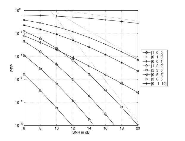
Figure 3: Monte-Carlo Simulation Results for $3\times 3$ $S=3$ case with $4$-QAM

For a rate $k_{c}/n_{c}$ binary convolutional code and a fixed Gray-encoded constellation labeling map in a BICMB system, BER $P_{b}$ can be bounded as

$$P_{b}\leq\frac{1}{k_{c}}\sum_{d=d_{free}}^{\infty}\sum_{i=1}^{W_{I}(d)}g(d,Q(d,i),\chi)$$ (40)

where $g(\cdot)$ is PEP corresponding to each error event, $W_{I}(d)$ denotes the total input weight of error events at Hamming distance $d$, and $Q$ is different for each error event. Since BER is dominated by PEP with the worst exponent term, the diversity order of a given BICMB system can be represented by

$$O_{diversity}=(M-Q_{max}+1)(N-Q_{max}+1)$$ (41)

where $Q_{max}$ is the maximum $Q$ among the whole set of $Q$’s corresponding to all of the error events.

V Relationship between $Q_{max}$ and code rate

The relationship between $Q_{max}$ and the code with rate $R_{c}$ is analyzed by using the same approach as in [15] which employes the Singleton bound to calculate the minimum distance of a non-binary block code. Let’s define $d_{E,s}(\mathbf{c},\mathbf{\hat{c}})$ as the Euclidean distance between the mapped symbols of the two codewords residing on the $s^{th}$ subchannel, $d_{E,s}(\mathbf{c},\mathbf{\hat{c}})=\sum_{k=1}^{L}|y_{k,s}-\hat{y}_{k,s}|^{2}$ where $y_{k,s}$ and $\hat{y}_{k,s}$ are symbols on the $s^{th}$ subchannel at the time index $k$ from the codeword $\mathbf{c}$ and $\mathbf{\hat{c}}$, respectively. If $\alpha_{s}$ is equal to zero, then all of the coded bits on the $s^{th}$ subchannel of the two codewords are the same. Since we assume that the consecutive bits are mapped over different symbols, the symbols corresponding to the same coded bits of the $s^{th}$ subchannel are also the same, resulting in $d_{E,s}(\mathbf{c},\mathbf{\hat{c}})=0$. Then, the parameter $Q$ can be viewed as an index to the first non-zero element in a vector $[d_{E,1}(\mathbf{c},\mathbf{\hat{c}})\quad d_{E,2}(\mathbf{c},\mathbf{\hat{c}})\quad\cdots\quad d_{E,S}(\mathbf{c},\mathbf{\hat{c}})]$. In the case of a pair of the codewords that has $S-1$ non-zero $d_{E,s}(\mathbf{c},\mathbf{\hat{c}})$’s, $Q$ can be $2$ because of the vector type $[0\,\times\,\times\,\cdots\,\times]$, or $1$ from $[\times\,0\,\times\,\times\,\cdots\,\times]$, $[\times\,\times\,0\,\times\,\times\,\cdots\,\times]$, $\cdots$, $[\times\,\times\,\times\,\cdots\,\times\,0]$, where $\times$ stands for non-zero value. In general, for a pair of the codewords that has $\delta_{H}$ non-zero $d_{E,s}(\mathbf{c},\mathbf{\hat{c}})$’s, $Q$ is bounded as

$$Q\leq S-\delta_{H}+1.$$ (42)

If we consider the $L$ symbols transmitted on each subchannel as a super-symbol over $\chi^{L}$, then the transmitted symbols for all the subchannels in a block can be viewed as a vector of length $S$ super-symbols. For convenience, we will call this vector of super-symbols as a symbol-wise codeword. We will now introduce a distance between $\mathbf{c}$ and $\mathbf{\hat{c}}$, which we will call $\delta_{H}$, as the number of non-zero elements in the vector $[d_{E,1}(\mathbf{c},\mathbf{\hat{c}})\quad d_{E,2}(\mathbf{c},\mathbf{\hat{c}})\quad\cdots\quad d_{E,S}(\mathbf{c},\mathbf{\hat{c}})]$. This distance is similar to the Hamming distance but it is between two non-binary symbol-wise codewords. By using the Singleton bound which is also applicable to non-binary codes, we can calculate the minimum distance of the symbol-wise codewords in a way similar to finding the minimum Hamming distance of binary codes. Let’s define $\mathcal{M}$ as the number of distinct symbol-wise codewords. Then we can see that $\mathcal{M}=2^{mLSR_{c}}$ from Fig. 1. Let $k$ $(0<k\leq S-1)$ denote the integer value satisfying $2^{mL(k-1)}<\mathcal{M}\leq 2^{mLk}$. Since $\mathcal{M}>2^{mL(k-1)}$, there necessarily exist two symbol-wise codewords whose $k-1$ elements are the same. From the Singleton bound [9], the minimum distance of these symbol-wise codewords $\delta_{H,min}$ is expressed as $\delta_{H,min}\leq S-k+1$. Since $2^{mLSR_{c}}\leq 2^{mL(S-\delta_{H,min}+1)}$, we get

$$\delta_{H,min}\leq S-\lceil S\cdot R_{c}\rceil+1$$ (43)

using the fact that $\delta_{H,min}$ is an integer value.

For a given BICMB system with $\delta_{H,min}$, it is true that the distance $\delta_{H}$ between any pair of the codewords is always larger than or equal to the minimum distance $\delta_{H,min}$. By combining the inequalities of $\delta_{H}\geq\delta_{H,min}$ and (42), we get $\delta_{H,min}\leq\delta_{H}\leq S-Q+1$, leading to the following inequality as

$$Q\leq S-\delta_{H,min}+1.$$ (44)

From the inequality (44), the maximum $Q$ among the whole set of $Q$’s can be found as

$$Q_{max}=S-\delta_{H,min}+1.$$ (45)

The inequality (43) and the equation (45) result in the following inequality as

$$Q_{max}\geq\lceil S\cdot R_{c}\rceil.$$ (46)

The relationship (46) can be supported by the examples in Section III where the $1/2$-rate convolutional code is used in $S=3$ BICMB system with different spatial de-multiplexers. Since $Q_{max}$ can be $2$ or $3$ according to (46), the rotating spatial de-multiplexer used to calculate $\mathbf{T}_{2}$ in (III) makes $Q_{max}$ equal to $2$ while that of $\mathbf{T}_{3}$ in (III) makes $Q_{max}$ equal to $3$. By considering the calculated diversity order of (41), the maximum diversity order for a given code rate BICMB system is achieved by choosing the convolutional encoder and the spatial de-multiplexer satisfying $Q_{max}=\lceil S\cdot R_{c}\rceil$. In this case, the maximum achievable diversity order is

$$O_{diversity}=(M-\lceil S\cdot R_{c}\rceil+1)(N-\lceil S\cdot R_{c}\rceil+1).$$ (47)

Based on (47), Fig. 4 depicts the relationship between the code rate $R_{c}$, the number of streams $S$, and the maximum achievable diversity order. The whole combinations of $S$ and $R_{c}$ are divided into the four regions each representing the maximum achievable diversity order. For example, such combinations as $(S$, $R_{c})$ $=$ $(2$, $1/2)$, $(2$, $1/3)$, $(2$, $1/4)$, $(3$, $1/3)$, $(3$, $1/4)$ in the region with the legend of $MN$ achieve the full diversity order of $MN$.

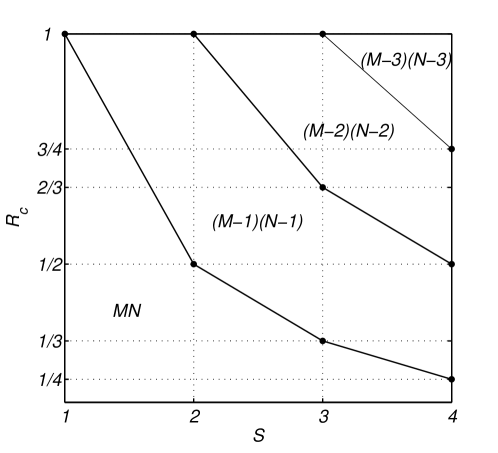
Figure 4: Multiplexing-Diversity-Rate Relationship

Since we assumed in the previous description that there exist the convolutional encoder and the spatial de-multiplexer which satisfy the relation $Q_{max}=\lceil S\cdot R_{c}\rceil$, we will show the specific design method of the interleaver from a given convolutional encoder to ensure the relation. The following method is not the unique solution to guarantee the maximum achievable condition, but simple to state the concept. Let’s consider a BICMB system with $S$ subchannels and the code rate $R_{c}=k_{c}/n_{c}$ convolutional code. Each of $P=LCM(n_{c},S)$ coded bits is distributed to the $S$ streams in the order specified by the interleaving pattern. Since each stream needs to be evenly employed for a period, $P/S$ coded bits are assigned on each stream. To guarantee $Q_{max}=\lceil S\cdot R_{c}\rceil$, it is sufficient to consider only the first branches that split from the zero state in one period because of the repetition property of the convolutional code. We incorporate the basic idea that once the $s^{th}$ stream is assigned to an error bit of the first branch, obviously, all of the error events containing that branch give $\alpha_{s}>0$, resulting in $Q\leq s$. By extending this idea, we can summarize the assignment procedure as

1. the lowest available subchannel is assigned to the error bit position of one of the first branches which have not yet assigned to any subchannel,

2. the procedure 1) is repeated until all of the first branches are assigned to one of the subchannels. If all of the first branches are assigned to one of the subchannels, the assignment procedure quits after the rest of subchannels are assigned randomly to the unassigned bit positions, subject to satisfying the rate condition on each subchannel.

We will explain the procedure above by using the example of Fig. 2 where $P=4$ and the number of available assignment for each subchannel is $P/S=1$. From the trellis, we can see there are $2$ first branches that split from the zero state for one period. According to the procedure above, we need to assign the best subchannel to one of the first branches. In this example, let’s assign it to the dummy variable $a$. This ensures $\alpha_{1}>0$ for all the error events stemming from this branch, resulting in $Q=1$. For the second branch connecting $X_{i}$ to $X_{11}$, we need to assign the next available lowest subchannel, which is $2$, to the dummy variable $c$. As a result, we can see that $Q\leq 2$ for the error events that share this branch. Since all of the first two branches are assigned, the unassigned dummy variables are allocated randomly with $3$ and $4$. This procedure assures that $Q_{max}$ is equal to $1$ or $2$ for this BICMB system. On the other hand, $Q_{max}\geq 2$ from the equation (46) resulting from the Singleton bound. Therefore, this method guarantees $Q_{max}=2$, which is the condition to achieve the maximum diversity order for the given convolutional code.

VI Simulation Results

To show the validity of the diversity order analysis in Section IV using the parameter $Q_{max}$ calculated by the method in Section III, BER against SNR are derived through a Monte-Carlo simulation. Fig. 5 shows BER performances for the cases corresponding to $\mathbf{T}_{1}$, $\mathbf{T}_{2}$, $\mathbf{T}_{3}$ in (III), (III), and (III). The well-known reference curves achieving the full diversity order of $MN$ are drawn from the Alamouti code for the $2\times 2$ case and $1/2$-rate orthogonal space-time block code (OSTBC) for the $3\times 3$ case [16]. From (III), $Q_{max}$ for $\mathbf{T}_{1}$ is found to be $1$ because $\alpha_{s}\geq 1$ for $s=1,2$ in all of the $\alpha$-vectors. In this case, as predicted by the analysis in [5], [6], the diversity order equals $4$ by calculating (41) with $M=N=2$. From the figure, we can see that BER curve for $\mathbf{T}_{1}$ is parallel to that of $2\times 2$ Alamouti code. Since $Q_{max}$ for $\mathbf{T}_{2}$ is $2$ due to the vector $[0\,5\,3]$, the calculated diversity order is $4$ in the case of $M=N=S=3$. This can be verified by Fig. 5, losing the full diversity order $9$. Although the same number of subchannels and the same convolutional code as for $\mathbf{T_{2}}$ are used, the different spatial de-multiplexer from that of $\mathbf{T_{2}}$, described in Section III for $\mathbf{T_{3}}$, gives no diversity gain at all. The reason for this is that the vector $[0\,0\,5]$ which can be observed from the transfer function in $\mathbf{T}_{3}$ makes $Q_{max}$ $3$ resulting in the calculated diversity order of $1$ in the equation (41) with $M=N=S=3$. This matches the simulation result.

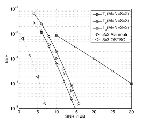
Figure 5: Simulation results for a $4$-state $1/2$-rate convolutional code with different spatial de-multiplexers. $4$-QAM is used for all of the curves.

Table I shows results of a computer search of the $\alpha$-vectors of BICMB with industry standard $64$-state convolutional codes and a simple rotating spatial de-multiplexer. The generator polynomials for rates $1/2$ and $1/3$ are $(133,171)$ and $(133,145,175)$ in octal, respectively. For the high rate codes such as $2/3$ and $3/4$, the perforation matrices in [12] are used from the $1/2$-rate original code. Instead of displaying the whole transfer functions, we present only three $\alpha$-vectors among such a number of dominant $\alpha$-vectors that lead to $Q_{max}$. The search results comply with the bound $Q_{max}\geq\lceil S\cdot R_{c}\rceil$ in (46) as was analyzed in Section V.

TABLE I: Search Results of the dominant $\alpha$-vectors for $64$-state convolutional codes

$S$	rate	$d_{free}$	dominant $\alpha$-vectors	$Q_{max}$
$2$	$1/2$	$10$	$[3\,\,7]$ $[4\,\,6]$ $[5\,\,5]$	$1$
	$2/3$	$6$	$[0\,\,12]$ $[0\,\,14]$ $[0\,\,15]$	$2$
	$3/4$	$5$	$[0\,\,8]$ $[0\,\,10]$ $[0\,\,12]$	$2$
$3$	$1/3$	$15$	$[3\,\,6\,\,6]$ $[5\,\,4\,\,6]$ $[4\,\,6\,\,6]$	$1$
	$1/2$	$10$	$[0\,\,7\,\,7]$ $[0\,\,8\,\,6]$ $[0\,\,9\,\,7]$	$2$
	$2/3$	$6$	$[0\,\,4\,\,5]$ $[0\,\,6\,\,3]$ $[0\,\,4\,\,6]$	$2$
	$3/4$	$5$	$[0\,\,0\,\,13]$ $[0\,\,0\,\,15]$ $[0\,\,0\,\,17]$	$3$

Fig. 6 shows the BER performance of the $2\times 2$ $S=2$ BICMB system with the $64$-state convolutional code and a simple rotating spatial de-multiplexer. The diversity orders of the systems with punctured codes are $1$ because both $Q_{max}$ values corresponding to the codes shown in Table I are $2$, while the system with the $1/2$-rate convolutional code, whose $Q_{max}$ is equal to $1$, achieves full diversity order of $4$.

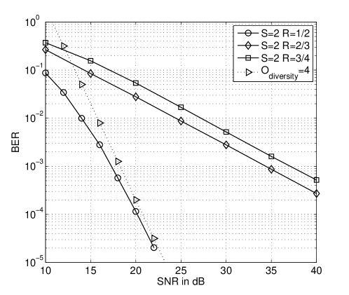
Figure 6: Simulation results for the $2\times 2$ case where $16$-QAM is used for all of the curves

As shown in Fig. 7, for a $3\times 3$ system with $3$ streams, only $1/3$-rate convolutional code achieves full diversity order of $9$ since other codes have $Q_{max}$ of larger than $1$ as given in Table I. The analytically calculated diversity orders by using (41) and Table I are $4$, $4$, $1$ for $1/2$, $2/3$, $3/4$ respectively, which can be easily verified from Fig. 7 by being compared with the asymptotes. For the rate-$3/4$ code with the same spatial de-multiplexer, reducing one stream improves the performance dramatically. The diversity order of this case is $4$ from the equation (41) with $M=N=3$ and $Q_{max}=2$.

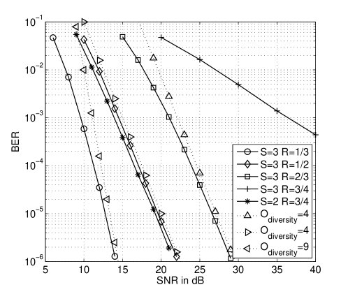
Figure 7: Simulation results for $3\times 3$ case where $16$-QAM is used for all of the curves

VII Conclusion

In this paper, we investigated the diversity order of BICMB when the interleaver does not meet the previously introduced design criteria. We introduced a method to calculate the $\alpha$-vectors from a given convolutional code and a spatial de-multiplexer by using a transfer function. By using this method, the $\alpha$-vectors that do not fulfill the full diversity order criteria are quantified. Then, the diversity behavior corresponding to the $\alpha$-vectors was analyzed through PEP calculation. The exponent of PEP between two codewords is $(M-Q+1)(N-Q+1)$ where $Q$ is the first index to the non-zero element in the $\alpha$-vector. Since BER is dominated by PEP with the smallest exponent, the diversity order is $(M-Q_{max}+1)(N-Q_{max}+1)$, where $Q_{max}$ is the maximum among $Q$’s corresponding to each $\alpha$-vector. We provided the simulation results that verify the analysis. We also showed that $Q_{max}$ is lower bounded by the product of the code rate and the number of streams. This result indicated that we need $R_{c}\leq 1/S$ to achieve the full diversity order of $NM$. [Proof of the smallest degree]

Since $r\left(\mu_{\ell(1)},\cdots,\mu_{\ell(K)}\right)$ is a product of the two polynomials as shown in (36), the smallest degree of $r\left(\mu_{\ell(1)},\cdots,\mu_{\ell(K)}\right)$ is a sum of the smallest degrees of each polynomial. Let’s denote $D_{g,smallest}$ as the smallest degree of the polynomial $g\left(\mu_{\ell(1)},\cdots,\mu_{\ell(K)}\right)$. It is easily found that all of the terms in (34) have the same degree. Therefore,

$$D_{g,smallest}=K(M-N)+K(K-1)$$ (48)

where the degree of $K(M-N)$ is contributed by the $K$ factors of the form $\mu_{\ell(k)}^{M-N}$, and $K(K-1)$ comes from the $\binom{K}{2}$ factors in the form of $\left(\mu_{\ell(k)}-\mu_{\ell(j)}\right)^{2}$.

To calculate the smallest degree of the polynomial $h\left(\mu_{\ell(1)},\cdots,\mu_{\ell(K)}\right)$, we first focus on the case of $\alpha_{1}=0$. The polynomial $p\left(\mu_{1},\cdots,\mu_{N}\right)$ in (28) has $N$ factors of the form $\mu_{i}^{M-N}$ and $\binom{N}{2}$ factors of the form $\left(\mu_{i}-\mu_{j}\right)^{2}$. The division by $g\left(\mu_{\ell(1)},\cdots,\mu_{\ell(K)}\right)$ makes the common factors eliminated, leaving $N-K$ and $\binom{N}{2}-\binom{K}{2}$ factors of the form $\mu_{i}^{M-N}$ and $\left(\mu_{i}-\mu_{j}\right)^{2}$, respectively. Hence, the resulting polynomial $p\left(\mu_{1},\cdots,\mu_{N}\right)/g\left(\mu_{\ell(1)},\cdots,\mu_{\ell(K)}\right)$ has degree

$$D_{h,org}=(N-K)(M-N)+N(N-1)-K(K-1).$$ (49)

The integration over $\mu_{i}$ for $1\leq i\leq\ell(1)-1$ in (35) makes the variables $\mu_{i}$, $1\leq i\leq\ell(1)-1$ vanish. Since all the terms in $p\left(\mu_{1},\cdots,\mu_{N}\right)/g\left(\mu_{\ell(1)},\cdots,\mu_{\ell(K)}\right)$ have different distributions on the degrees of the individual variables although they have the same degree as an entire term, the smallest degree of $h\left(\mu_{\ell(1)},\cdots,\mu_{\ell(K)}\right)$ is determined by the term which has the largest degree of the vanishing variables of $p\left(\mu_{1},\cdots,\mu_{N}\right)/g\left(\mu_{\ell(1)},\cdots,\mu_{\ell(K)}\right)$. It’s not necessary to find all the terms with the largest degree of the vanishing variables. Instead, we can see that one of those terms, whose degree is $D_{h,org}$, includes the following factors

$$\prod\limits_{i=1}^{\ell(1)-1}\mu_{i}^{M-N}\prod\limits_{j>i}^{N}\mu_{i}^{2}.$$ (50)

In this case, the degree for the vanishing variables in (50) is

$$D_{h,vanishing}=(\ell(1)-1)(M-N)+2N(\ell(1)-1)-\ell(1)(\ell(1)-1)$$ (51)

where $(\ell(1)-1)(M-N)$ is contributed by the $\ell(1)-1$ factors of the form $\mu_{i}^{M-N}$, and the rest of the degrees are calculated from the factors of the form $\mu_{i}^{2}$.

Finally, the integration over $\mu_{i}$ for $\ell(1)+1\leq i\leq N$ accumulates the degree of the current variables and adds up to the degree of the corresponding $\mu_{k},k\in\Upsilon$, where an ordered set $\Upsilon$ is defined as $\left\{i:\alpha_{i}>0\,\textrm{for }1\leq i\leq S\right\}$. In addition, during the each integration, the degree increases by $1$ due to the fact that $\int_{0}^{\mu_{i}}\mu_{i+1}^{n}d\mu_{i+1}=\mu_{i}^{n+1}/(n+1)$. Since $\ell(1)-1$ variables from original $N-K$ variables of integration vanished in $h\left(\mu_{\ell(1)},\cdots,\mu_{\ell(K)}\right)$, the degree to be added by the remaining variables of integration is

$$D_{h,added}=N-K-\ell(1)+1.$$ (52)

The smallest degree of $r\left(\mu_{\ell(1)},\cdots,\mu_{\ell(K)}\right)$ is now ready to be calculated, which is

$$D_{r,smallest} =D_{g,smallest}+D_{h,smallest}$$

$$=D_{g,smallest}+\left(D_{h,org}-D_{h,vanishing}+D_{h,added}\right)$$

$$=(M-\ell(1)+1)(N-\ell(1)+1)-K$$ (53)

where $D_{h,org}-D_{h,vanishing}$ stands for the degree of the remaining non-vanishing variables of the term that leads to the smallest degree of $h\left(\mu_{\ell(1)},\cdots,\mu_{\ell(K)}\right)$.

In the case of $\alpha_{1}>0$, the integrations over the variables $\mu_{i}$, $1\leq i\leq\ell(1)-1$ in (35) do not exist. Contrary to the case of $\alpha_{1}=0$, no variable vanishes, resulting in $D_{h,vanishing}=0$, and $D_{h,added}=N-K$. Equation (53) holds true for $\alpha_{1}>0$ since $\ell(1)=1$ in this case. Therefore, for any case of $\alpha_{1}$, the smallest degree of the polynomial $r\left(\mu_{\ell(1)},\cdots,\mu_{\ell(K)}\right)$ is $(M-\ell(1)+1)(N-\ell(1)+1)-K$.

References

- [1] H. Jafarkhani, Space-Time Coding: Theory and Practice. Cambridge University Press, 2005.
- [2] D. P. Palomar, J. M. Cioffi, and M. A. Lagunas, “Joint tx-rx beamforming design for multicarrier MIMO channels: A unified framework for convex optimization,” IEEE Trans. Signal Process., vol. 51, no. 9, pp. 2381–2401, September 2003.
- [3] E. Sengul, E. Akay, and E. Ayanoglu, “Diversity analysis of single and multiple beamforming,” IEEE Trans. Commun., vol. 54, no. 6, pp. 990–993, June 2006.
- [4] L. G. Ordonez, D. P. Palomar, A. Pages-Zamora, and J. R. Fonollosa, “High-SNR analytical performance of spatial multiplexing MIMO systems with CSI,” IEEE Trans. Signal Process., vol. 55, no. 11, pp. 5447–5463, November 2007.
- [5] E. Akay, E. Sengul, and E. Ayanoglu, “Bit interleaved coded multiple beamforming,” IEEE Trans. Commun., vol. 55, no. 9, pp. 1802–1811, September 2007.
- [6] E. Akay, H. J. Park, and E. Ayanoglu, “On bit-interleaved coded multiple beamforming,” arXiv: 0807.2464. [Online]. Available: http://arxiv.org
- [7] J. G. Proakis, Digital Communications, 4th ed. McGraw-Hill, 2000.
- [8] D. Haccoun and G. Begin, “High-rate punctured convolutional codes for Viterbi and sequential decoding,” IEEE Trans. Commun., vol. 37, no. 11, pp. 1113–1125, November 1989.
- [9] R. C. Singleton, “Maximum distance q-nary codes,” IEEE Trans. Inf. Theory, vol. 10, no. 2, pp. 116–118, April 1964.
- [10] E. Sengul, H. J. Park, and E. Ayanoglu, “Bit-interleaved coded multiple beamforming with imperfect CSIT,” IEEE Trans. Commun., to appear.
- [11] J. Conan, “The weight spectra of some short low-rate convolutional codes,” IEEE Trans. Commun., vol. 32, no. 9, pp. 1050–1053, September 1984.
- [12] G. Begin, D. Haccoun, and C. Paquin, “Further results on high-rate punctured convolutional codes for viterbi and sequential decoding,” IEEE Trans. Commun., vol. 38, no. 11, pp. 1922–1928, November 1990.
- [13] A. Edelman, “Eigenvalues and condition numbers of random matrices,” Ph.D. dissertation, MIT, Cambridge, MA, 1989.
- [14] A. M. Tulino and S. Verdú, Random Matrix Theory and Wireless Communications. Now Publishers, 2004.
- [15] R. Knopp and P. A. Humblet, “On coding for block fading channels,” IEEE Trans. Inf. Theory, vol. 46, no. 1, pp. 189–205, January 2000.
- [16] V. Tarokh, H. Jafarkhani, and A. R. Calderbank, “Space-time block coding for wireless communications: Performance results,” IEEE J. Sel. Areas Commun., vol. 17, no. 3, pp. 451–460, March 1999.