Abstract

In this article, we calculate the contribution from the nonfactorizable soft hadronic matrix element to the decay $B^{0}\rightarrow\chi_{c1}\pi^{0}$ with the light-cone QCD sum rules. The numerical results show that its contribution is rather large and should not be neglected. The total amplitudes lead to a branching fraction which is in agreement with the experimental data marginally.

PACS number: 13.25.Hw, 12.39.St, 12.38.Lg

Key Words: Light-cone QCD sum rule, $B$-decay, nonfactorizable hadronic matrix element

1 Introduction

Recently, the Belle Collaboration measured the branching fraction for the Cabibbo- and color-suppressed decay $B^{0}\to\chi_{c1}\pi^{0}$ based on a data sample of $657\times 10^{6}$ $B\overline{B}$ events collected at the $\Upsilon(4S)$ resonance with the Belle detector at the KEKB asymmetric-energy $e^{+}e^{-}$ collider [1]. The signal is $40\pm 9$ events with a significance of $4.7\sigma$ including systematic uncertainties, and the branching fraction is about $(1.12\pm 0.25\pm 0.12)\times 10^{-5}$.

The decay takes place through the process $b\to dc\bar{c}$ (or more precise $\bar{b}\to\bar{d}c\bar{c}$, they relate with each other by charge conjunction, in this article, we calculate the amplitudes for the process $b\to dc\bar{c}$, then take charge conjunction to obtain the branching fraction.) at the quark-level [2]. If the leading order tree diagram dominates, the time-dependent CP-violating asymmetries are predicted to be the same as the ones in the $b\to sc\bar{c}$ decays [3]. The time-dependent CP-violation parameters for the similar decay $B^{0}\to J/\psi\pi^{0}$ have been measured by the Belle [4, 5] and Babar [6, 7, 8] Collaborations. The deviation of the CP-violating asymmetries from those expectations may indicate non-negligible contributions from the penguin amplitudes or new physics.

The quantitative understanding of the $B$-decays depends on our knowledge about the nonperturbative hadronic matrix elements of the operators entering the effective weak Hamiltonian [2]. In recent years, great progresses have been made in this aspect, such as the generalized factorization approach [9, 10], the QCD factorization approach [11, 12], the perturbative QCD [13, 14], the soft-collinear effective theory [15], etc. Factorization of the hadronic matrix elements has been proved to hold in the leading order in many processes.

The effects of the soft gluons which violate factorization are supposed of order $O(\frac{\Lambda_{QCD}}{m_{b}})$ and neglected in the QCD-improved factorization studies [11, 12], however, no theoretical work has ever proved that they are small quantities. For the color-suppressed $B$ to charmonia decays, there may be significant impacts of the nonfactorizable soft contributions.

In Ref.[16], Khodjamirian introduce a technique based on the light-cone QCD sum rules to estimate the nonfactorizable soft contributions, where the soft gluon effects are represented by the quark-antiquark-gluon distribution amplitudes of the light mesons, the hadronic matrix element appears as a part of the hadronic dispersion relation for the correlation function. Thereafter, the light-cone QCD sum rules are applied to study the nonfactorizable hadronic matrix elements in the $B$-decays due to the soft gluons exchanges [17, 18, 19, 20, 21, 22, 23, 24, 25, 26, 27].

It is interesting to study the nonfactorizable soft contributions in the decay $B^{0}\to\chi_{c1}\pi^{0}$ with the light-cone QCD sum rules.

The article is organized as follows: the factorizable contributions from the effective weak Hamiltonian are derived in Sec.2; the soft hadronic matrix element $\langle\chi_{c1}\pi^{0}|{\cal\widetilde{O}}(0)|B\rangle$ is calculated with the light-cone sum rules approach in Sec.3; numerical results are presented in Sec.4; the section 5 is reserved for conclusion.

2 Effective weak Hamiltonian and factorizable contributions

The effective weak Hamiltonian for the $b\rightarrow dc\bar{c}$ decay modes can be written as (for detailed discussion of the effective weak Hamiltonian, one can consult Ref. [2])

$$H_{w}=\frac{G_{F}}{\sqrt{2}}\left\{V_{cb}V_{cd}^{*}\left[C_{1}(\mu){\cal O}_{1}+C_{2}(\mu){\cal O}_{2}\right]-V_{tb}V_{td}^{*}\sum_{i=3}^{10}C_{i}{\cal O}_{i}\right\}\,,$$ (1)

where $V_{ij}$’s are the CKM matrix elements, $C_{i}$’s are the Wilson coefficients calculated at the renormalization scale $\mu\sim O(m_{b})$ and the relevant operators ${\cal O}_{i}$ are given by

$${\cal O}_{1} = (\overline{d}_{\alpha}b_{\beta})_{V-A}(\overline{c}_{\beta}c_{\alpha})_{V-A}\,,$$

$${\cal O}_{2} = (\overline{d}_{\alpha}b_{\alpha})_{V-A}(\overline{c}_{\beta}c_{\beta})_{V-A}\,,$$

$${\cal O}_{3(5)} = (\overline{d}_{\alpha}b_{\alpha})_{V-A}\sum_{q}(\overline{q}_{\beta}q_{\beta})_{V-A(V+A)}\,,$$

$${\cal O}_{4(6)} = (\overline{d}_{\alpha}b_{\beta})_{V-A}\sum_{q}(\overline{q}_{\beta}q_{\alpha})_{V-A(V+A)}\,,$$ (2)

where we have neglected the Wilson coefficients $C_{7},C_{8},C_{9},C_{10}$ due to their small values. We can reorganize the color-mismatched quark fields into color singlet states by Fierz transformation, and express the effective weak Hamiltonian $H_{w}$ in the following form,

$$H_{w} = \frac{G_{F}}{\sqrt{2}}\left\{V_{cb}V_{cd}^{*}\left[\left(C_{2}(\mu)+\frac{C_{1}(\mu)}{3}\right){\cal O}_{2}+2C_{1}(\mu){\cal\widetilde{O}}_{2}\right]\right.$$ (3)

$$-V_{tb}V_{td}^{*}\left[\left(C_{3}(\mu)+\frac{C_{4}(\mu)}{3}\right){\cal O}_{3}+2C_{4}(\mu){\cal\widetilde{O}}_{3}\right]$$

$$\left.-V_{tb}V_{td}^{*}\left[\left(C_{5}(\mu)+\frac{C_{6}(\mu)}{3}\right){\cal O}_{5}+2C_{6}(\mu){\cal\widetilde{O}}_{5}\right]\right\}\,,$$

where

$${\cal\widetilde{O}}_{2} = (\overline{c}\gamma_{\mu}(1-\gamma_{5})\frac{\lambda_{a}}{2}c)(\overline{d}\gamma^{\mu}(1-\gamma_{5})\frac{\lambda_{a}}{2}b)\,,$$

$${\cal\widetilde{O}}_{3} = (\overline{c}\gamma_{\mu}(1-\gamma_{5})\frac{\lambda_{a}}{2}c)(\overline{d}\gamma^{\mu}(1-\gamma_{5})\frac{\lambda_{a}}{2}b)\,,$$

$${\cal\widetilde{O}}_{5} = (\overline{c}\gamma_{\mu}(1+\gamma_{5})\frac{\lambda_{a}}{2}c)(\overline{d}\gamma^{\mu}(1-\gamma_{5})\frac{\lambda_{a}}{2}b)\,,$$ (4)

and $\lambda^{a}$’s are $SU(3)$ Gell-Mann matrices.

The factorizable matrix elements $\langle\chi_{c1}(p)\pi^{0}(-q)|H_{w}|B(p-q)\rangle$ can be parameterized as $\epsilon^{*}\cdot qA_{f}$,

$$\epsilon^{*}\cdot qA_{f} = \frac{G_{F}}{\sqrt{2}}\left\{-V_{cb}V_{cd}^{*}\left[C_{2}(\mu)+\frac{C_{1}(\mu)}{3}\right]\right.$$ (5)

$$\left.+V_{tb}V_{td}^{*}\left[C_{3}(\mu)+\frac{C_{4}(\mu)}{3}-C_{5}(\mu)-\frac{C_{6}(\mu)}{3}\right]\right\}$$

$$\langle\chi_{c1}(p)|\overline{c}\gamma_{\mu}\gamma_{5}c|0\rangle\langle\pi^{0}(-q)|\overline{d}\gamma^{\mu}b|B(p-q)\rangle\,.$$

The $\chi_{c1}$ meson decay constant is defined by $\langle\chi_{c1}(p)|\overline{c}(0)\gamma_{\mu}\gamma_{5}c(0)|0\rangle=f_{\chi_{c1}}m_{\chi_{c1}}\epsilon_{\mu}^{*}$. The $B-\pi^{0}$ form-factor can be parameterized as

$$-\sqrt{2}\langle\pi^{0}(q)|\bar{d}\gamma_{\mu}b|B(P)\rangle = f(p^{2})(P+q)_{\mu}-[f(p^{2})-f_{0}(p^{2})]\frac{m_{B}^{2}-m_{\pi}^{2}}{p^{2}}p_{\mu}\,,$$ (6)

the form-factors $f(p^{2})$ and $f_{0}(p^{2})$ can be estimated with the light-cone sum rules approach, here we take the value $f(m_{\chi_{c1}}^{2})=0.62$ [28].

The concise expression for the factorizable matrix elements can be written as

$$A_{f} = -G_{F}f_{\chi_{c1}}m_{\chi_{c1}}f(m_{\chi_{c1}}^{2})\left\{V_{cb}V_{cd}^{*}\left[C_{2}(\mu)+\frac{C_{1}(\mu)}{3}\right]-\right.$$ (7)

$$\left.V_{tb}V_{td}^{*}\left[C_{3}(\mu)-C_{5}(\mu)+\frac{C_{4}(\mu)-C_{6}(\mu)}{3}\right]\right\}\,.$$

3 Light-cone QCD sum rules for the nonfactorizable hadronic matrix element $\langle\chi_{c1}\pi^{0}|{\cal\widetilde{O}}(0)|B\rangle$

In the following, we apply the approach developed in Ref.[16] for the $B\rightarrow\pi\pi$ channel to estimate the contribution from the soft-gluon exchanges in the decay $B^{0}\to\chi_{c1}\pi^{0}$. We write down the correlation function $\Pi_{\rho}(p,q,k)$ firstly,

$$\Pi_{\rho}(p,q,k) = i^{2}\,\int d^{4}xe^{-i(p-q)x}\int d^{4}ye^{i(p-k)y}\langle 0|T\{J_{\rho}(y){\cal\widetilde{O}}(0)J_{5}(x)\}|\pi^{0}(q)\rangle\,,$$ (8)

where ${\cal\widetilde{O}}={\cal\widetilde{O}}_{2}$, the currents $J_{\rho}=\bar{c}\gamma_{\rho}\gamma_{5}c$ and $J_{5}=m_{b}\bar{b}i\gamma_{5}d$ interpolate the mesons $\chi_{c1}$ and $B$, respectively.

The correlation function $\Pi_{\rho}(p,q,k)$ can be calculated by the operator product expansion approach near the light-cone $x^{2}\sim y^{2}\sim(x-y)^{2}\sim 0$ in perturbative QCD theory. It is function of three independent momenta chosen to be $q$, $p-k$ and $k$. We introduce the unphysical momentum $k$ in order to avoid that the $B$ meson has the same four-momentum before ($p-q$) and after the decay ($P$), and thus avoid a continuum of light contributions in the dispersion relation in the $B$-channel. The independent kinematical invariants can be taken as $(p-q)^{2}$, $(p-k)^{2}$, $q^{2}$ , $k^{2}$, $P^{2}=(p-k-q)^{2}$ and $p^{2}$. We set $k^{2}=0$ and take $q^{2}=m_{\pi}^{2}=0$, neglecting the small corrections of order $O(m_{\pi}^{2}/m_{B}^{2})$. The momentum $p^{2}$ is kept undefined for the moment in order to make the derivation of the sum rules without restriction. Its value is going to be set later in this section, and chosen to be $p^{2}=m_{\chi_{c1}}^{2}$. The values of $(p-k)^{2}$, $(p-q)^{2}$ and $P^{2}$ should be spacelike and large in order to stay far away from the hadronic thresholds in the $B$ and $\chi_{c1}$ channels. All together, we have

$$q^{2}=k^{2}=0,\;p^{2}=m_{\chi_{c1}}^{2},\;|(p-k)|^{2}\gg\Lambda_{QCD},|(p-q)|^{2}\gg\Lambda_{QCD},|P|^{2}\gg\Lambda_{QCD}\,\,.$$

The correlation function $\Pi_{\rho}(p,q,k)$ can be decomposed as

$$\Pi_{\rho}(p,q,k) = (p-k)_{\rho}\Pi+q_{\rho}\widetilde{\Pi}_{1}+k_{\rho}\widetilde{\Pi}_{2}+\epsilon_{\rho\alpha\beta\sigma}q^{\alpha}p^{\beta}k^{\sigma}\widetilde{\Pi}_{3}\,,$$ (9)

due to Lorentz covariance.

According to the basic assumption of quark-hadron duality in the QCD sum rules [29, 30], we insert a complete set of intermediate states with the same quantum numbers as the current operators $J_{\mu}(y)$ and $J_{5}(x)$ into the correlation function $\Pi_{\rho}(p,q,k)$ to obtain the hadronic representation. After isolating the pole terms of the ground state mesons $\chi_{c1}$ and $B$, we get the following result,

$$\Pi_{\rho} = \frac{\langle 0|J_{\rho}(0)|\chi_{c1}(p-k)\rangle}{m^{2}_{\chi_{c1}}-(p-k)^{2}}\langle\chi_{c1}(p-k)|{\cal\widetilde{O}}(0)|B(p-q)\rangle|\pi^{0}(q)\rangle\frac{\langle B(p-q)|J_{5}(0)|0\rangle}{m^{2}_{B}-(p-q)^{2}}$$

$$+\cdots,$$

$$= \frac{f_{\chi_{c1}}m_{\chi_{c1}}\epsilon_{\rho}}{m^{2}_{\chi_{c1}}-(p-k)^{2}}\frac{f_{B}m^{2}_{B}}{m^{2}_{B}-(p-q)^{2}}\langle\chi_{c1}(p-k)\pi^{0}(-q)|{\cal\widetilde{O}}(0)|B(p-q)\rangle+\cdots,$$

$$= \frac{f_{\chi_{c1}}m_{\chi_{c1}}}{m^{2}_{\chi_{c1}}-(p-k)^{2}}\frac{f_{B}m^{2}_{B}}{m^{2}_{B}-(p-q)^{2}}q_{\alpha}\left[-g_{\alpha\rho}+\frac{(p-k)_{\alpha}(p-k)_{\rho}}{(p-k)^{2}}\right]A_{n}+\cdots,$$

where we have used the definition $\langle\chi_{c1}(p-k)\pi^{0}(-q)|{\cal\widetilde{O}}(0)|B(p-q)\rangle=\epsilon^{*}\cdot qA_{n}$, and do not show the contributions from the higher resonances and continuum states above the corresponding thresholds explicitly, they can be written in terms of dispersion integrals and the spectral density can be approximated by the quark-hadron duality ansatz.

Now we carry out the operator product expansion near the light-cone to obtain the representation at the level of quark-gluon degrees of freedom. Let us write down the propagator of a massive quark in the external gluon field in the Fock-Schwinger gauge firstly [31],

$$S_{ij}(x,y) = i\int\frac{d^{4}k}{(2\pi)^{4}}e^{-ik(x-y)}\Bigg{\{}\frac{\not\!k+m}{k^{2}-m^{2}}\delta_{ij}-\int\limits_{0}^{1}dv\,g_{s}\,G^{\mu\nu}_{ij}(vx+(1-v)y)$$ (11)

$$\Big{[}\frac{1}{2}\frac{\not\!k+m}{(k^{2}-m^{2})^{2}}\sigma_{\mu\nu}-\frac{1}{k^{2}-m^{2}}v(x-y)_{\mu}\gamma_{\nu}\Big{]}\Bigg{\}}\,,$$

where $G^{\mu\nu}_{a}$ is the gluonic field strength, $g_{s}$ denotes the strong coupling constant.

Substituting the above $b$ and $c$ quark propagators into the correlation function $\Pi_{\rho}$, and completing the corresponding integrals, we can obtain the hadronic spectral density at the level of quark-gluon degrees of freedom. In calculation, the following three-particle $\pi^{0}$ light-cone distribution amplitudes are useful,

$$-\sqrt{2}\langle 0|\bar{d}(0)\sigma_{\mu\nu}\gamma_{5}G_{\alpha\beta}(vy)d(x)|\pi^{0}(q)\rangle = if_{3\pi}\left[q_{\alpha}q_{\mu}g_{\beta\nu}+q_{\beta}q_{\nu}g_{\alpha\mu}-q_{\beta}q_{\mu}g_{\alpha\nu}-\right.$$

$$\left.q_{\alpha}q_{\nu}g_{\beta\mu}\right]\int{\cal D}\alpha_{i}\phi_{3\pi}(\alpha_{i})e^{-iq(x\alpha_{1}+yv\alpha_{3})}\,,$$

$$-\sqrt{2}\langle 0|\bar{d}(0)i\gamma_{\mu}\tilde{G}_{\alpha\beta}(vy)d(x)|\pi^{0}(q)\rangle = f_{\pi}q_{\mu}\frac{q_{\alpha}x_{\beta}-q_{\beta}x_{\alpha}}{qx}\int{\cal D}\alpha_{i}\widetilde{\phi}_{\parallel}(\alpha_{i})e^{-iq(x\alpha_{1}+yv\alpha_{3})}+$$

$$f_{\pi}(g_{\mu\alpha}^{\perp}q_{\beta}-g_{\mu\beta}^{\perp}q_{\alpha})\int{\cal D}\alpha_{i}\widetilde{\phi}_{\perp}(\alpha_{i})e^{-iq(x\alpha_{1}+yv\alpha_{3})}\,,$$

$$-\sqrt{2}\langle 0|\bar{d}(0)\gamma_{\mu}\gamma_{5}{G}_{\alpha\beta}(vy)d(x)|\pi^{0}(q)\rangle = f_{\pi}q_{\mu}\frac{q_{\alpha}x_{\beta}-q_{\beta}x_{\alpha}}{qx}\int{\cal D}\alpha_{i}{\phi}_{\parallel}(\alpha_{i})e^{-iq(x\alpha_{1}+yv\alpha_{3})}+$$

$$f_{\pi}(g_{\mu\alpha}^{\perp}q_{\beta}-g_{\mu\beta}^{\perp}q_{\alpha})\int{\cal D}\alpha_{i}{\phi}_{\perp}(\alpha_{i})e^{-iq(x\alpha_{1}+yv\alpha_{3})}\,,$$

where $\tilde{G}_{\alpha\beta}=\frac{1}{2}\epsilon_{\alpha\beta\rho\sigma}G^{\rho\sigma}$, ${\cal D}\alpha_{i}=d\alpha_{1}d\alpha_{2}d\alpha_{3}\delta(1-\alpha_{1}-\alpha_{2}-\alpha_{3})$, $g_{\alpha\beta}^{\perp}=g_{\alpha\beta}-\frac{x_{\alpha}q_{\beta}+x_{\beta}q_{\alpha}}{qx}$. The twist-3 and twist-4 light-cone distribution amplitudes can be parameterized as

$$\phi_{3\pi}(\alpha_{i}) = 360\alpha_{1}\alpha_{2}\alpha_{3}^{2}\left[1+\frac{\omega_{3}}{2}(7\alpha_{3}-3)\right]\,,$$

$$\phi_{\perp}(\alpha_{i}) = 30\delta^{2}(\alpha_{1}-\alpha_{2})\alpha_{3}^{2}\left[\frac{1}{3}+2\epsilon(1-2\alpha_{3})\right]\,,$$

$$\phi_{\parallel}(\alpha_{i}) = 120\delta^{2}\epsilon(\alpha_{1}-\alpha_{2})\alpha_{1}\alpha_{2}\alpha_{3}\,,$$

$$\widetilde{\phi}_{\perp}(\alpha_{i}) = 30\delta^{2}\alpha_{3}^{2}(1-\alpha_{3})\left[\frac{1}{3}+2\epsilon(1-2\alpha_{3})\right]\,,$$

$$\widetilde{\phi}_{\parallel}(\alpha_{i}) = -120\delta^{2}\alpha_{1}\alpha_{2}\alpha_{3}\left[\frac{1}{3}+\epsilon(1-3\alpha_{3})\right]\,,$$ (13)

the nonperturbative parameters in the light-cone distribution amplitudes can be estimated with the QCD sum rules [34, 35, 36].

After carrying out the operator product expansion near the light-cone, we obtain the following expression for the correlation function $\Pi$ ,

$$\Pi = \frac{m_{b}f_{3\pi}}{2\pi^{2}}\int_{0}^{1}dv\int_{0}^{1}dt\int{\cal D}\alpha_{i}\frac{\phi_{3\pi}(\alpha_{i})q\cdot(p-k)\left[tvq\cdot k+2(1-t)(1-v)q\cdot p\right]}{\left\{m_{b}^{2}-[p-q(1-\alpha_{1})]^{2}\right\}\left\{\widetilde{m}_{c}^{2}-(p-k-v\alpha_{3}q)^{2}\right\}}$$

$$+\frac{m^{2}_{b}f_{\pi}}{4\pi^{2}}\int_{0}^{1}dv\int_{0}^{1}dt\int{\cal D}\alpha_{i}\frac{q\cdot(p-k)}{\left\{m_{b}^{2}-[p-q(1-\alpha_{1})]^{2}\right\}\left\{\widetilde{m}_{c}^{2}-(p-k-v\alpha_{3}q)^{2}\right\}}$$

$$\left\{(1-2t)\left[2(1-v)\phi_{\perp}(\alpha_{i})-(1-2v)\phi_{\parallel}(\alpha_{i})\right]+2(1-v)\widetilde{\phi}_{\perp}(\alpha_{i})-\widetilde{\phi}_{\parallel}(\alpha_{i})\right\}\,,$$

where $\widetilde{m}_{c}^{2}=\frac{m_{c}^{2}}{t(1-t)}$.

In order to suppress the contributions from the high resonances and continuum states, we perform n-th derivative with respect to the momentum $(p-k)^{2}$ to obtain stable n-th moment sum rules and Borel transform with respect to the momentum $(p-q)^{2}$ in the $B$-channel to obtain the Borel sum rules, then match with Eq.(10), finally we obtain the sum rule for the nonfactorizable soft matrix element,

$$A_{n} = \frac{2m_{\chi_{c1}}}{f_{B}f_{\chi_{c1}}m^{2}_{B}\left[m_{\chi_{c1}}^{2}-P^{2}\right]}\int_{4m^{2}_{c}}^{s_{0}}ds\left\{\frac{f_{3\pi}m_{b}}{4\pi^{2}}\int_{t_{i}}^{t_{f}}dt\int_{\alpha_{0}}^{1}d\alpha\int_{\alpha_{c}}^{\alpha}d\beta\right.$$ (15)

$$\left.\phi_{3\pi}(1-\alpha,\alpha-\beta,\beta)\left[\frac{t\alpha_{c}}{2\beta}(P^{2}-s-\frac{m_{b}^{2}-m_{\chi_{c1}}^{2}}{\alpha})-(1-t)(1-\frac{\alpha_{c}}{\beta})\frac{m_{b}^{2}-m^{2}_{\chi_{c1}}}{\alpha}\right]\right.$$

$$+\frac{f_{\pi}m_{b}^{2}}{8\pi^{2}}\int_{t_{i}}^{t_{f}}dt\int_{\alpha_{0}}^{1}d\alpha\int_{\alpha_{c}}^{\alpha}d\beta\left[2(1-\frac{\alpha_{c}}{\beta})\widetilde{\phi}_{\perp}-\widetilde{\phi}_{\parallel}+\right.$$

$$\left.\left.(1-2t)\left[2(1-\frac{\alpha_{c}}{\beta})\phi_{\perp}-(1-\frac{2\alpha_{c}}{\beta})\phi_{\parallel}\right]\right](1-\alpha,\alpha-\beta,\beta)\right\}$$

$$\exp\left(\frac{\alpha m_{B}^{2}+m^{2}_{\chi_{c1}}(1-\alpha)-m^{2}_{b}}{\alpha M^{2}}\right)\left(\frac{m^{2}_{\chi_{c1}}+Q_{0}^{2}}{s+Q_{0}^{2}}\right)^{n+1}\frac{1}{\alpha\beta}\,,$$

where

$$t_{i}=\frac{1}{2}\left(1-\sqrt{1-\frac{4m_{c}^{2}}{s}}\right)\,, t_{f}=\frac{1}{2}\left(1+\sqrt{1-\frac{4m_{c}^{2}}{s}}\right)\,,$$

$$\alpha_{c}=\frac{t(1-t)s-m_{c}^{2}}{t(1-t)(s-P^{2})}\,, \alpha_{0}=\frac{m_{b}^{2}-m^{2}_{\chi_{c1}}}{s_{B}-m^{2}_{\chi_{c1}}}\,,$$ (16)

and $Q_{0}^{2}=4m_{c}^{2}\xi$. In calculation, $P^{2}$ is chosen to be large space-like squared momentum ($|P^{2}|\sim m_{b}^{2}$) in order to stay far away from the hadronic thresholds, the value of $\alpha_{c}$ is a small positive quantity but not always small enough to be safely neglected, we perform the following approximation for the $\beta$ integral,

$$\int_{\alpha_{c}}^{\alpha}d\beta G(s,x,\alpha,\beta)=\left\{\int^{\alpha}_{0}-\int^{\alpha_{c}}_{0}\right\}d\beta G(s,x,\alpha,\beta)\,,$$ (17)

here $G$ is an abbreviation for the integral functions and can be written as

$$G(s,x,\alpha,\beta) = A\phi_{3\pi}(1-\alpha,\alpha-\beta,\beta)+B\widetilde{\phi}_{\parallel}(1-\alpha,\alpha-\beta,\beta)+C\widetilde{\phi}_{\perp}(1-\alpha,\alpha-\beta,\beta)$$

$$+D\phi_{\parallel}(1-\alpha,\alpha-\beta,\beta)+E\phi_{\perp}(1-\alpha,\alpha-\beta,\beta)\,,$$

$A,B,C,D,E$ are formal notations. We can expand the light-cone distribution amplitudes $\phi_{3\pi}$, $\widetilde{\phi}_{\parallel}$, $\widetilde{\phi}_{\perp}$, $\phi_{\parallel}$ and $\phi_{\perp}$ in terms of Taylor series of $\beta$, for example,

$$\phi_{3\pi}(1-\alpha,\alpha-\beta,\beta) = \phi_{3\pi}(1-\alpha,\alpha-\beta,\beta)|_{\beta=0}+\frac{\partial}{\partial\beta}\phi_{3\pi}(1-\alpha,\alpha-\beta,\beta)|_{\beta=0}\beta$$ (18)

$$+\frac{1}{2}\frac{\partial^{2}}{\partial\beta^{2}}\phi_{3\pi}(1-\alpha,\alpha-\beta,\beta)|_{\beta=0}\beta^{2}+\cdots\,,$$

and continue $P^{2}$ into the timelike region analytically, $P^{2}=m^{2}_{B}$, then complete the integral $\int^{\alpha_{c}}_{0}d\beta G(s,x,\alpha,\beta)$. This procedure ensures the disappearance of the unphysical momentum $k$ from the ground state contribution and enables the extraction of the physical matrix element due to the simultaneous conditions, $P^{2}=m_{B}^{2}$ and $(p-q)^{2}=m_{B}^{2}$.

The explicit expression for the physical hadronic matrix element is lengthy due to the re-summation of all the Taylor series of $\beta$, here we show only the leading terms explicitly,

$$A_{n} = \frac{2m_{\chi_{c1}}}{f_{B}f_{\chi_{c1}}m^{2}_{B}\left[m_{\chi_{c1}}^{2}-m_{B}^{2}\right]}\int_{4m^{2}_{c}}^{s_{0}}ds\left\{\frac{f_{3\pi}m_{b}}{4\pi^{2}}\int_{t_{i}}^{t_{f}}dt\int_{\alpha_{0}}^{1}d\alpha\int_{0}^{\alpha}d\beta\right.$$ (19)

$$\phi_{3\pi}(1-\alpha,\alpha-\beta,\beta)\left[\frac{t\alpha_{c}}{2\beta}(m_{B}^{2}-s-\frac{m_{b}^{2}-m_{\chi_{c1}}^{2}}{\alpha})-(1-t)(1-\frac{\alpha_{c}}{\beta})\frac{m_{b}^{2}-m^{2}_{\chi_{c1}}}{\alpha}\right]$$

$$+\frac{f_{\pi}m_{b}^{2}}{8\pi^{2}}\int_{t_{i}}^{t_{f}}dt\int_{\alpha_{0}}^{1}d\alpha\int_{0}^{\alpha}d\beta\left[2(1-\frac{\alpha_{c}}{\beta})\widetilde{\phi}_{\perp}-\widetilde{\phi}_{\parallel}+\right.$$

$$\left.\left.(1-2t)\left[2(1-\frac{\alpha_{c}}{\beta})\phi_{\perp}-(1-\frac{2\alpha_{c}}{\beta})\phi_{\parallel}\right]\right](1-\alpha,\alpha-\beta,\beta)\right\}$$

$$\exp\left(\frac{\alpha m_{B}^{2}+m^{2}_{\chi_{c1}}(1-\alpha)-m^{2}_{b}}{\alpha M^{2}}\right)\left(\frac{m^{2}_{\chi_{c1}}+Q_{0}^{2}}{s+Q_{0}^{2}}\right)^{n+1}\frac{1}{\alpha\beta}$$

$$-\frac{2m_{\chi_{c1}}}{f_{B}f_{\chi_{c1}}m^{2}_{B}\left[m_{\chi_{c1}}^{2}-m_{B}^{2}\right]}\int_{4m^{2}_{c}}^{s_{0}}ds\left\{\frac{f_{3\pi}m_{b}}{4\pi^{2}}\int_{t_{i}}^{t_{f}}dt\int_{\alpha_{0}}^{1}d\alpha\int_{0}^{\alpha_{c}}d\beta\right.$$

$$\phi_{3\pi}(1-\alpha,\alpha-\beta,\beta)\mid_{\beta=0}\left[\frac{t\alpha_{c}}{2\beta}(m_{B}^{2}-s-\frac{m_{b}^{2}-m_{\chi_{c1}}^{2}}{\alpha})-\right.$$

$$\left.(1-t)(1-\frac{\alpha_{c}}{\beta})\frac{m_{b}^{2}-m^{2}_{\chi_{c1}}}{\alpha}\right]$$

$$+\frac{f_{\pi}m_{b}^{2}}{8\pi^{2}}\int_{t_{i}}^{t_{f}}dt\int_{\alpha_{0}}^{1}d\alpha\int_{0}^{\alpha_{c}}d\beta\left[2(1-\frac{\alpha_{c}}{\beta})\widetilde{\phi}_{\perp}-\widetilde{\phi}_{\parallel}+\right.$$

$$\left.\left.(1-2t)\left[2(1-\frac{\alpha_{c}}{\beta})\phi_{\perp}-(1-\frac{2\alpha_{c}}{\beta})\phi_{\parallel}\right]\right](1-\alpha,\alpha-\beta,\beta)\mid_{\beta=0}\right\}$$

$$\exp\left(\frac{\alpha m_{B}^{2}+m^{2}_{\chi_{c1}}(1-\alpha)-m^{2}_{b}}{\alpha M^{2}}\right)\left(\frac{m^{2}_{\chi_{c1}}+Q_{0}^{2}}{s+Q_{0}^{2}}\right)^{n+1}\frac{1}{\alpha\beta}+\cdots\,\,.$$

In performing the $\beta$ integral $\int_{0}^{\alpha_{c}}$, we need only the values of the light-cone distribution amplitudes $\phi_{3\pi}$, $\widetilde{\phi}_{\parallel}$, $\widetilde{\phi}_{\perp}$, $\phi_{\parallel}$, $\phi_{\perp}$ and their derivations at zero momentum fraction i.e. $\beta=0$, there are no problems with negative partons (quarks and gluons) momentum fractions. The analytical continuation of $P^{2}$ to its positive value ends up with an unavoidable theoretical uncertainty, if only a few terms of the Taylor series are taken. However, with the re-summation to all orders of $\beta$ in Eq.(19), the assumption of quark-hadron duality is still applicable in the case of heavy meson final states.

4 Numerical results

The input parameters are taken as $V_{cd}=-0.230$, $V_{cb}=41.2\times 10^{-3}$, $V_{tb}=1.0$, $V_{td}=8.1\times 10^{-3}$, $m_{\chi_{c1}}=3.511\,\rm{GeV}$, $m_{B}=5.2795\,\rm{GeV}$ [37], $f_{B}=0.18\,\rm{GeV}$, $s_{B}=35\pm 2\,{\rm GeV}^{2}$ [32], $f_{\chi_{c1}}=0.335\,\rm{GeV}$ [33], $s_{0}=(16.0\pm 0.5)\,{\rm GeV}^{2}$ [30], $f_{\pi}=0.13\,\rm{GeV}$, $m_{b}=(4.7\pm 0.1)\,\rm{GeV}$, $m_{c}=(1.35\pm 0.05)\,\rm{GeV}$, $f_{3\pi}=(0.45\pm 0.15)\times 10^{-2}\,\rm{GeV}^{2}$, $\omega_{3}=-1.5\pm 0.7$, $\delta^{2}=(0.18\pm 0.06)\,\rm{GeV}^{2}$, $\varepsilon=\frac{21}{8}(0.2\pm 0.1)$ [34, 35, 36] at the energy scale about $\mu=1\,\rm{GeV}$.

The parameters $n$ and $M^{2}$ must be carefully chosen to warrant the high resonances and continuum states to be suppressed and obtain a reliable perturbative QCD calculation. The stable region for the Borel parameter $M^{2}$ is found in the interval $M^{2}=11\pm 2\,{\rm GeV}^{2}$, which is known from the $B$ channel QCD sum rules [32]. In the charmonium channels, we usually perform n-th derivative and take n-th moment sum rules to satisfy the stability criteria [30], the ideal interval is $n=4-6$. The parameter $\xi$ is usually allowed to take values larger than 1 for the $P$-wave charmonia, we observe the best interval is $\xi=1.8-2.6$.

The nonfactorizable soft contributions come from the three-particle twist-3 and twist-4 $\pi^{0}$ light-cone distribution amplitudes, however, present knowledge about those distribution amplitudes is rather poor. The uncertainties of the nonperturbative parameters $f_{3\pi}$, $\omega_{3}$, $\delta^{2}$ and $\varepsilon$ are large, about $(33-50)\%$, the nonfactorizable soft contributions $A_{n}$ can be simplified into the following form,

$$A_{n} = y_{1}f_{3\pi}+y_{2}f_{3\pi}\omega_{3}+y_{3}\delta^{2}+y_{4}\delta^{2}\varepsilon\,,$$ (20)

where the $y_{i}$ are numerical coefficients not shown explicitly. The uncertainties origin from the nonperturbative parameters $f_{3\pi}$, $\omega_{3}$, $\delta^{2}$ and $\varepsilon$ are rather large, even out of control. We take the same treatment as Refs.[20, 21, 22, 23, 26], and neglect the corresponding uncertainties, it weakens the predictive ability. The uncertainties origin from other parameters ($s_{B}$, $s_{0}$, $m_{b}$, $m_{c}$, $n$, $\xi$, etc) are less than $22\%$, we take into account them with the formula $\Delta=\sqrt{\sum_{i}\left(\frac{\partial f}{\partial x_{i}}\right)^{2}(x_{i}-\bar{x}_{i})^{2}}$, where the $f$ denote the nonfactorizable soft contributions, the $x_{i}$ denote the input parameters.

Taking into account the next-to-leading order Wilson coefficients calculated in the naive dimensional regularization scheme [2] for $\mu=\overline{m_{b}}(m_{b})=4.40{\rm\,GeV}$ and $\Lambda_{\overline{\rm MS}}^{(5)}=225\,{\rm MeV}$,

$$\qquad C_{1}(\overline{m_{b}}(m_{b}))=1.082\,,\qquad C_{2}(\overline{m_{b}}(m_{b}))=-0.185\,,\qquad C_{3}(\overline{m_{b}}(m_{b}))=0.014\,,$$

$$\qquad C_{4}(\overline{m_{b}}(m_{b}))=-0.035\,,\qquad C_{5}(\overline{m_{b}}(m_{b}))=0.009\,,\qquad C_{6}(\overline{m_{b}}(m_{b}))=-0.041\,,$$ (21)

finally we obtain the numerical ratio $R$ between the contributions from the nonfactorizable and factorizable hadronic matrix elements, which is shown in Fig.1,

$$R = \frac{\sqrt{2}C_{1}(\mu)\langle\chi_{c1}(p)\pi^{0}(-q)|{\cal{\widetilde{O}}}(0)|B(p-q)\rangle}{-\left[C_{2}(\mu)+\frac{C_{1}(\mu)}{3}\right]f_{\chi_{c1}}m_{\chi_{c1}}f(m^{2}_{\chi_{c1}})}=0.68^{+0.20}_{-0.16}\,\,.$$ (22)

The nonfactorizable soft contributions are rather large and they must be included in analyzing the branching fraction. The total amplitudes lead to the branching fraction,

$$Br(B^{0}\to\chi_{c1}\pi^{0})=1.41^{+0.35}_{-0.25}\times 10^{-5}\,,$$ (23)

which is in agreement with the experimental data $(1.12\pm 0.25\pm 0.12)\times 10^{-5}$ marginally [1].

The factorizable contributions of the operator ${\cal O}_{2}(0)$ can be analyzed in the same way with the correlation function $\widehat{\Pi}_{\rho}(p,q,k)$,

$$\widehat{\Pi}_{\rho} = i^{2}\,\int d^{4}xe^{-i(p-q)x}\int d^{4}ye^{i(p-k)y}\langle 0|T\{J_{\rho}(y){\cal O}_{2}(0)J_{5}(x)\}|\pi^{0}(q)\rangle$$ (24)

$$= \int d^{4}xe^{-i(p-q)x}\langle 0|T[\overline{d}(0)\gamma^{\mu}b(0)J_{5}(x)]|\pi^{0}(q)\rangle\int d^{4}ye^{i(p-k)y}\langle 0|T[J_{\rho}(y)J_{\mu}(0)]|0\rangle$$

$$\propto (p-k)_{\rho}f\left((p-k)^{2}\right)\times f_{\chi_{c1}}^{2}+\cdots\,.$$

The contributions of the soft gluons can be absorbed into the $B\to\pi^{0}$ form-factor $f\left((p-k)^{2}\right)$ or the decay constant $f_{\chi_{c1}}$, and differ from the sum rules for the operator ${\cal{\widetilde{O}}}(0)$ greatly, where the contributions of the soft gluons are nonfactorizable, so we are free of double-counting.

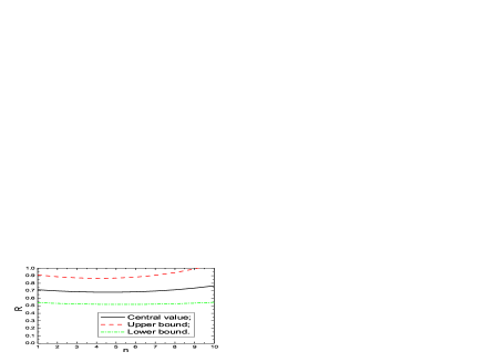
Figure 1: The ratio $R$ between the contributions from the nonfactorizable and factorizable hadronic matrix elements.

5 Conclusion

In this article, we calculate the contributions from the nonfactorizable soft hadronic matrix element $\langle\chi_{c1}(p)\pi^{0}(-q)|{\cal{\widetilde{O}}}(0)|B(p-q)\rangle$ to the decay $B^{0}\rightarrow\chi_{c1}\pi^{0}$ with the light-cone QCD sum rules. The numerical results show that its contribution is rather large and should not be neglected. The total amplitudes lead to a branching fraction which is in agreement with the experimental data marginally.

References

[1] R. Kumar et al, arXiv:0809.1778.
[2] G. Buchalla, A. J. Buras and M. E. Lautenbacher,
Rev. Mod. Phys. 68 (1996) 1125.
[3] A. B. Carter and A. I. Sanda, Phys. Rev. D23 (1981) 1567.
[4] S. U. Kataoka et al, Phys. Rev. Lett. 93 (2004) 261801.
[5] S. E. Lee et al, Phys. Rev. D77 (2008) 071101.
[6] B. Aubert et al, Phys. Rev. Lett. 91 (2003) 061802.
[7] B. Aubert et al, Phys. Rev. D74 (2006) 011101.
[8] B. Aubert et al, Phys. Rev. Lett. 101 (2008) 021801.
[9] A. Ali, G. Kramer and C. D. Lu, Phys. Rev. D58 (1998) 094009.
[10] Y. H. Chen et al, Phys. Rev. D60 (1999) 094014.
[11] M. Beneke et al, Nucl. Phys. B591 (2000) 313.
[12] M. Beneke et al, Nucl. Phys. B606 (2001) 245.
[13] Y. Y. Keum, H. n. Li and A. I. Sanda, Phys. Lett. B504 (2001) 6.
[14] Y. Y. Keum, H. n. Li and A. I. Sanda, Phys. Rev. D63 (2001) 054008.
[15] C. W. Bauer et al, Phys. Rev. D63 (2001) 114020.
[16] A. Khodjamirian, Nucl. Phys. B605 (2001) 558.
[17] A. Khodjamirian, T. Mannel and P. Urban, Phys. Rev. D67 (2003) 054027.
[18] B. Melic, Phys. Rev. D68 (2003) 034004.
[19] A. Khodjamirian, T. Mannel and B. Melic, Phys. Lett. B571 (2003)
75.
[20] L. Li, Z. G. Wang and T. Huang, Phys. Rev. D70 (2004) 074006.
[21] B. Melic, Phys. Lett. B591 (2004) 91.
[22] T. Huang et al, Phys. Rev. D70 (2004) 094013.
[23] N. Mahajan, Phys. Lett. B634 (2006) 240.
[24] A. Khodjamirian et al, Phys. Rev. D72 (2005) 094012.
[25] X. Y. Wu et al, Chin. Phys. Lett. 19 (2002) 1596.
[26] J. Y. Cui and Z. H. Li, Eur. Phys. J. C38 (2004) 187.
[27] Z. H. Li, Z. Q. Su and J. Y. Cui, hep-ph/0602231.
[28] P. Ball and R. Zwicky, Phys. Rev. D71 (2005) 014015.
[29] M. A. Shifman, A. I. Vainshtein and V. I. Zakharov,
Nucl. Phys. B147 (1979) 385, 448.
[30] L. J. Reinders, H. Rubinstein and S. Yazaki, Phys. Rept. 127
(1985) 1.
[31] V. M. Belyaev et al, Phys. Rev. D51 (1995) 6177.
[32] A. Khodjamirian and R. Ruckl, Adv. Ser. Direct. High Energy Phys. 15 (1998) 345.
[33] V. A. Novikov et al, Phys. Rept. 41 (1978) 1.
[34] V. M. Braun and I. E. Filyanov, Z. Phys. C48 (1990) 239.
[35] V. L. Chernyak and A. R. Zhitnitsky, Phys. Rept. 112 (1984)
173.
[36] P. Ball, V. M. Braun and A. Lenz, JHEP 0605 (2006) 004.