Dark Matter Structures In The Deep Lens Survey

Abstract

We present a regularized maximum likelihood weak lensing reconstruction of the Deep Lens Survey F2 field (4 $\rm{deg^{2}}$). High signal-to-noise ratio peaks in our lensing significance map appear to be associated with possible projected filamentary structures. The largest apparent structure extends for over a degree in the field and has contributions from known optical clusters at three redshifts $(z\sim 0.3,0.43,0.5)$. Noise in weak lensing reconstructions is known to potentially cause “false positives”; we use Monte Carlo techniques to estimate the contamination in our sample, and find that 10-25% of the peaks are expected to be false detections. For significant lensing peaks we estimate the total signal-to-noise ratio of detection using a method that accounts for pixel-to-pixel correlations in our reconstruction. We also report the detection of a candidate relative underdensity in the F2 field with a total signal-to-noise ratio of $\sim 5.5$.

1 Introduction

The mass function of galaxy clusters is a well known probe of cosmological parameters (Haiman et al., 2001). Since cluster mass is not a direct observable other proxies such as optical galaxy richness (Koester et al., 2007), X-ray temperature (Rosati et al., 2002), the Sunyaev-Zel’dovich decrement (Carlstrom et. al., 2002), or weak gravitational lensing (Schneider, 1996) are used to trace the mass distribution. To produce accurate constraints on cosmological parameters the mass-observable conversion must be properly calibrated in order to avoid potential biases. With weak lensing, mass overdensities are selected from maps of the projected mass density and peaks of mass are identified as a function of their signal-to-noise ratio. The observable in this case is the weak lensing ‘shear’ which is independent of baryonic physics, and theoretically well understood. This is a major strength that weak lensing has over other methods. Known limitations of this method are projection effects due to large scale structure (Hennawi & Spergel, 2005; White et al., 2002) which can produce spurious detections, a low peak detection significance, complicated point-spread function (PSF) corrections, and the observational expense (since it requires deep imaging). In spite of these limitations, forecasts for future imaging surveys predict that this method will still provide large samples of shear-selected galaxy clusters which will allow for constraints on cosmological parameters, including dark energy (Marian & Bernstein, 2006). In addition to individual clusters, studies have also pointed out that the global statistics of dark matter peaks in weak lensing maps can be used to put constraints on cosmology (Jain & Van Waerbeke, 2000). Within a given dataset cosmological information from peak statistics could also play a complementary role in breaking degeneracies in cosmological parameters from studies of cosmic shear (Gavazzi & Soucail, 2007).

The current generation of deep optical imaging surveys are creating the first ever maps of the dark matter distribution with weak lensing. In Wittman et al. (2006) we presented preliminary maps from the Deep Lens Survey (DLS), covering a total of area of $8$ $\rm{deg}^{2}$ spread over five fields. Initial maps from the Canada-France-Hawaii Telescope Legacy survey covering four separate $1$ $\rm{deg}^{2}$ fields were presented in Gavazzi & Soucail (2007). Recently, results from the Hubble Space Telescope COSMOS 2 $\rm{deg}^{2}$ field were reported in Massey et al. (2007). To reconstruct the projected mass density ($\kappa$) in these surveys from weak lensing, all of these studies have implemented a ‘direct’ reconstruction method based on or related to the technique of Kaiser & Squires (1993). This reconstruction method is computationally efficient but has a number of known limitations; for instance, it requires setting an arbitrary smoothing scale, and it is difficult to incorporate other lensing effects such as magnification (Seitz et al., 1998). Several different reconstruction techniques have been developed to overcome these issues, the most promising of which advocate reconstructing the deflection potential ($\psi$) on a grid rather than directly determining $\kappa$. These techniques have primarliy been applied to pointed observations of individual clusters, for instance in Jee et al. (2007) or Bradac et al. (2006). In this study we use a regularized maximum likelihood technique to reconstruct the projected mass distribution over a wide area, four square degree field from the DLS.

Our paper is organized as follows: In $\S\ref{sec:data}$ details of the imaging data, PSF correction, and the source galaxies used in our analysis are presented. In $\S\ref{sec:analysis}$ the maximum likelihood algorithm used in our reconstruction and its application to the DLS are discussed. In $\S\ref{sec:masspeaks}$ the structures observed in the lensing reconstruction are presented along with their likely optical counterparts. In $\S\ref{sec:discussion}$ the expected false peak rate due to lensing shape noise is discussed as well as our method of determining the total signal-to-noise ratio of lensing peaks. In $\S\ref{sec:summary}$ our results are summarized and we discuss future directions of our work.

2 Data

The DLS is a deep imaging survey of five widely separated four square degree fields (F1-F5) in $BVRz^{\prime}$. Fields in the DLS were selected in a blind manner the only restrictions were to avoid bright foreground galaxies, known low redshift clusters ($z\lesssim 0.1$), and areas of high extinction (Wittman et al., 2002). A primary motivation for this was to create an unbiased shear selected sample of clusters. In this study we restrict our analysis to the F2 field centered on $\rm{R.A.}=09^{\rm{h}}19^{\rm{m}}32.4^{\rm{s}}$, $\rm{decl.}=+30^{\circ}00\arcmin 00\arcsec$. Observations of the F2 field were carried out using the MOSAIC I imager (Muller et al., 1998) on the Kitt Peak Mayall 4m telescope. Observations of F2 began at Kitt Peak in 1999 November and ended in 2004 November. This was the first DLS field and to have complete imaging. The observing strategy for the DLS is to split each field into a $3\times 3$ grid of $40\arcmin\times 40\arcmin$ subfields. Each completed subfield consists of twenty 900s $R$ band exposures, and twenty 600s exposures in each of the $BVz^{\prime}$ filters. The $R$ band is used as the primary filter to measure galaxy shapes for weak lensing, and observations were only carried out in this filter when the seeing FWHM was $<0.9\arcsec$. The remaining filters ($BVz^{\prime}$) are primarily used to measure photometric redshifts of source galaxies, however these are not used in our current analysis.

For our lensing analysis the shapes of background galaxies are measured from the co-added $R$ band subfield frames. A detailed discussion of the DLS weak lensing pipeline is given in Wittman et al. (2006) here we provide a brief overview. Basic reductions such as flat fielding and bias are performed using the IRAF package MSCRED. The MOSAIC cameras each consist of eight individual CCD detectors, and the PSF in each detector is determined by identifying stars from the stellar locus in magnitude-size space. We fit the spatial variation of the PSF in each detector using a third order polynomial, and a $3\times 3$ rounding kernel is used to circularize the PSF as in Fischer & Tyson (1997). The PSF corrected $R$ band images of each subfield are co-added using our custom software DLSCOMBINE (Wittman et al., 2006). The final co-added subfield images reach a depth of $R\sim 26$.

To initially detect objects in each subfield image we use the SExtractor (Bertin & Arnouts, 1996) package. Shapes for detected objects are then remeasured with adaptive moments using ELLIPTO (Smith et al., 2001; Heymans, 2006), which is a partial implementation of the algorithm of Bernstein & Jarvis (2002). Objects which triggered error flags in ELLIPTO were removed since these are objects where adaptive moments did not converge or indicated a problem with shape measurement. We also rejected objects which triggered SExtractor flags indicating a fatal error occured during shape measurement, the object contained a saturated pixel, or the object was too close the edge of the image. For our analysis we use source galaxies in the magnitude range $22.0<R<25.5$, where the number counts in the field peak at $R\sim 25.5$. We include only galaxies with ELLIPTO size $>1.25\times\rm{PSF}$ at the position of each galaxy. The maximum ELLIPTO size is set at $20.0$ $\rm{pixel^{2}}$ in order to eliminate potential low redshift, low surface brightness galaxies from our sample. Our size and magnitude cuts produce a sample of source galaxies that each have a signal-to-noise ratio $\gtrsim 15$. We also reject objects whose observed ellipticity is $e>0.6$, as these are likely superpositions of objects (Wittman et al., 2000). The dilution (or seeing) correction is performed using simulations described in $\S\ref{sec:reg}$. This is chosen over the analytic dilution correction described for the ELLITPO method in Heymans (2006), since it has been pointed out that this correction does not correctly incorporate the kurtosis of the PSF (Hirata & Seljak, 2003). The final subfield catalogs were stitched together to create a supercatalog of source galaxies for the F2 field. This catalog contains $\sim 328,000$ galaxies over the field, or $\sim 23$ galaxies $\rm{arcmin^{-2}}$.

Our current source galaxy catalog is not the same catalog used in Wittman et al. (2006) or Khiabanian & Dell’Antonio (2008). In both of these studies the catalog was restricted to brighter galaxies $(R<25)$ with larger galaxy sizes than we used here. This work uses a catalog with a factor of two more source galaxies than was used in Khiabanian & Dell’Antonio (2008).

3 Weak Lensing Analysis

3.1 Formalism

In the thin lens approximation the mapping of light from the source plane $\vec{\beta}$ to image plane $\vec{\theta}$ is given by the lens equation $\vec{\beta}=\vec{\theta}-\vec{\alpha}(\vec{\theta})$. The deflection angle $\vec{\alpha}$ of light due to a two dimensional Newtonian deflection potential $\psi$ of a lens is given by

$$\vec{\alpha}(\vec{\theta})=\vec{\bigtriangledown}\psi.$$ (1)

The surface mass density ($\kappa$) of the lens can be calculated directly from the deflection potential by

$$\kappa=\frac{\Sigma}{\Sigma_{crit}}=\frac{1}{2}(\psi_{11}+\psi_{22}),$$ (2)

where subscripts on $\psi$ refer to the partial derivatives $\psi_{ij}\equiv\frac{\partial^{2}\psi}{\partial\theta_{i}\partial\theta_{j}}$. Here the critical surface mass density ($\Sigma_{crit}$) is given by

$$\Sigma_{crit}=\frac{c^{2}}{4\pi G}\frac{D_{s}}{D_{d}D_{ds}},$$ (3)

where $D_{d}$, $D_{s}$, and $D_{ds}$ are the angular diameter distances to the lens, source, and between the lens and source respectively. The tidal gravitational field of the lens, or shear, is described in complex notion by $\gamma=\gamma_{1}+\rm{i}\gamma_{2}$ where the shear components are given by

$$\begin{array}[]{c}\gamma_{1}=\frac{1}{2}(\psi_{11}-\psi_{22})\\ \\ \gamma_{2}=\psi_{12}=\psi_{21}\\ \end{array}$$ (4)

and the complex reduced shear is given by $g=\gamma/(1-\kappa)$ (Schneider et al., 2000). For a more detailed discussion of lensing we refer the reader to Kochanek et al. (2005).

3.2 Regularized Maximum-Likelihood Reconstruction

Maximum likelihood methods for weak lensing cluster mass reconstruction were first demonstrated in Bartelmann et al. (1996). Several variants of this algorithm have since been proposed, for instance the methods described in Bridle et al. (1998) and Seitz et al. (1998). To produce a weak lensing convergence map of the F2 field we use a regularized maximum likelihood approach based on the method developed by Seitz et al. (1998) with improvements described in Khiabanian & Dell’Antonio (2008). In this technique the deflection potential in the field is determined over a grid, and the convergence map is generated directly from the deflection potential map using equation $(\ref{eqn:kappa})$.

To produce a convergence map with dimensions $N_{x}\times N_{y}$, a grid of the deflection potential with dimensions $(2N_{x}+4)\times(2N_{y}+4)$ is used. The twice larger grid is required here to fix the ringing effects in the projected mass maps caused by second order numerical differentiation of the deflection potential. The extra rows and columns are needed to compute $\kappa$ and $\gamma$ using second order finite differencing. With this method we minimize the function $\mathcal{F}$,

$$\mathcal{F}=\frac{1}{2}\chi^{2}+\lambda\mathcal{R},$$ (5)

where $\lambda$ is the regularization coefficient, and $\mathcal{R}$ is the regularization function. The $\chi^{2}$ term is determined from

$$\chi^{2}=\frac{1}{N_{g}}\sum_{k=1}^{N_{g}}\frac{(\epsilon_{k}-<\epsilon>(\textbf{x}_{k}))^{2}}{\sigma_{\epsilon}},$$ (6)

where $N_{g}$ is the number of source galaxies, $\epsilon_{k}$ is the complex ellipticity of a galaxy at position $x_{k}$, and $<\epsilon>$ is the expected ellipticity at $x_{k}$. We compute the expected ellipticity distribution and the dispersion $\sigma_{\epsilon}$, as a function of reduced shear from simulations (Khiabanian & Dell’Antonio, 2008). The ellipticity distribution in our simulations is based on the measured distribution from the Hubble Ultra Deep Field (Beckwith et al., 2006). We regularize $\chi^{2}$ using a zeroth-order regularization function given by

$$\mathcal{R}=\sum_{m=1}^{N_{x}}\sum_{n=1}^{N_{y}}(\kappa_{mn}-p_{mn})^{2}$$ (7)

where $\kappa_{mn}$ is the convergence at a grid point and $p_{mn}$ is the prior. This form of the regularization function is chosen for simplicity, but also ensures the smoothness of the reconstruction. The regularization coefficient, $\lambda$, in $\mathcal{F}$ represents a compromise between the best fit $\chi^{2}$ and the closest match to the prior. We minimize the function $\mathcal{F}$ using the conjugate gradient method from Press et al. (1992).

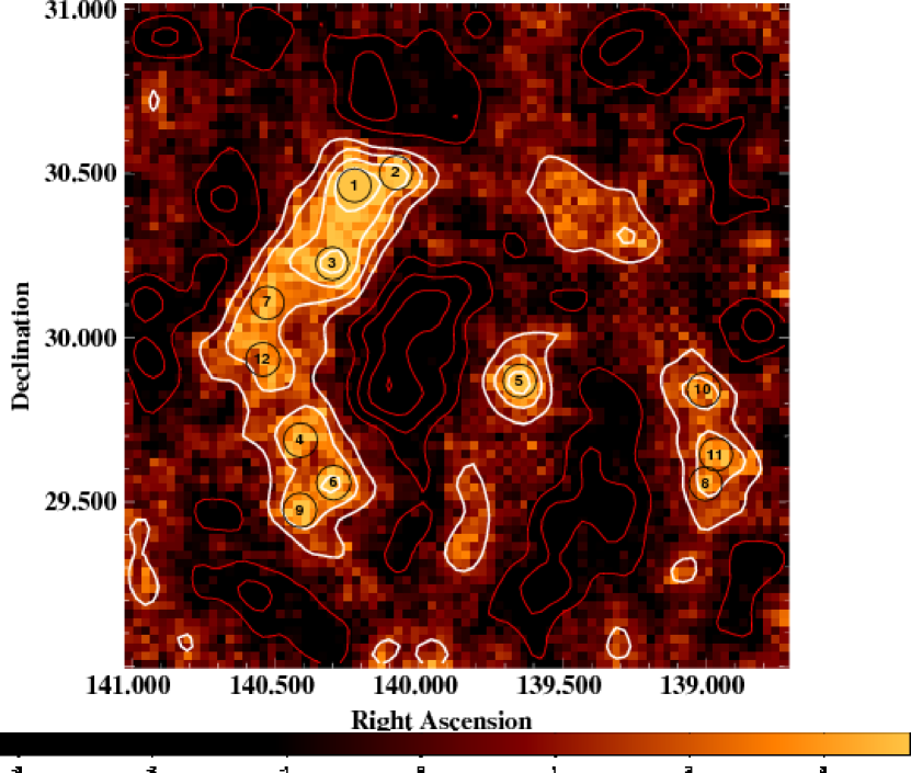
Figure 1: Weak lensing $\kappa-\rm{S/N}$ map of the F2 field centered on $\rm{R.A.}=09^{\rm{h}}19^{\rm{m}}32.4^{\rm{s}}$, $\rm{decl.}=+30^{\circ}00\arcmin 00\arcsec$. Postive contours of signal-to-noise ratio (white) are overlaid and enclose the $4,2,3,$ and $1\sigma$ regions; negative contours (red) enclose the $-4,-3,-2,$ and $-1\sigma$ regions. Black circles indicate the positions of the most significant peaks ($\nu>3.5$) with the rank of each peak shown at the center of each circle.

Our reconstruction proceeds at a series of different resolutions, beginning with a coarse $20\times 20$ grid of the potential and a completely uniform prior. This outputs a coarse potential which is used to create a convergence map. The resulting convergence map is smoothed and used as a prior to the next level of resolution. Using a smoothed prior has been shown to produce more accurate reconstructions (Seitz et al., 1998; Lucy, 1994). As described in Khiabanian & Dell’Antonio (2008) we choose the regularization coefficient at each of the higher resolution reconstructions by minimizing $\mathcal{F}$ (eq. 5) with multiple values of $\lambda$ (between 0 and 10) along with minimizing only $\mathcal{R}$ (eq. 7). We scale $\chi^{2}$ to values between 0 and 1, using its lowest value obtained when $\lambda=0$ and its highest value obtained when only $\mathcal{R}$ is minimized. Similarly, we scale $\mathcal{R}$ to values between 0 and 1. The intersection of the scaled $\chi^{2}$ vs $\mathcal{R}$ curve and the scaled line $\chi^{2}=\mathcal{R}$ determines the proper value of the regularization coefficient. This processes of producing maps at a given resolution and determining the proper regularization coefficient is repeated for three resolutions of the convergence map $(20\times 20$, $40\times 40$, $80\times 80$), until the final map resolution is achieved. Our final convergence map has dimensions of $80\times 80$ with a plate scale of $1\arcmin.5$ $\rm{pixel^{-1}}$. The resulting signal-to-noise ratio map (convergence map divided by the rms map) is shown in Figure 1. The rms map ($\kappa_{\rm{rms}}$) is described further in $\S\ref{sec:peaks}$.

4 Dark Matter Peaks in F2

4.1 $\kappa$ Signal-To-Noise Ratio Map

We search for lensing peaks in the F2 field by first creating a $\kappa$ signal-to-noise ratio map (henceforth $\kappa-\rm{S/N}$ map). As in Miyazaki et al. (2007) we construct a $\kappa_{\rm{rms}}$ map using 100 Monte Carlo realizations of the original source galaxy catalog. We note here that half as many realizations could have been used and the following results would not have changed.

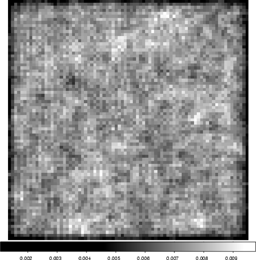
Figure 2: The $\kappa_{\rm{rms}}$ noise map based on 100 Monte Carlo realizations of the F2 field. Each individual Monte Carlo map is created by shuffling the source galaxy catalog positions and ellipticity components. A maximum likelihood $\kappa$ map is made for each individual Monte Carlo realization. Each pixel in the $\kappa_{\rm{rms}}$ map represents the $1\sigma$ error at this point over the set of Monte Carlo reconstructions.

In each realization, the position and ellipticity components of each galaxy are decoupled and randomly assigned to new galaxies. Shuffling the source catalog in this manner is useful since it preserves the real variation in background galaxy source density. For each shuffled source catalog, a maximum likelihood $\kappa$ map is created using the same regularization coefficients at each resolution as was used to create our original $\kappa$ map (Khiabanian & Dell’Antonio, 2008). From the resulting set of 100 Monte Carlo maps we created the $\kappa_{\rm{rms}}$ map shown in Figure 2. Each pixel in this map represents the $1\sigma$ standard deviation at this point over the set of Monte Carlo reconstructions. A $\kappa-\rm{S/N}$ map for F2 is made by dividing the original $\kappa$ map by the $\kappa_{\rm{rms}}$ map (Figure 1). Contours in the $\kappa-\rm{S/N}$ map range from a peak signal-to-noise ratio ($\nu$) of $1.0-6.0$; negative contours have been omitted here for clarity.

We detect peaks in the $\kappa-\rm{S/N}$ map using the SExtractor package (Bertin & Arnouts, 1996). Peaks are separated by setting the minimum contrast parameter in SExtractor to 0 which separates all possible peaks. We measure peaks relative to a zero background level and use the height of each peak to approximate the signal-to-noise ratio of detection. We set the minimum area for detection at 9 contiguous pixels and the minimum threshold for detection at 0.01. Our definition of a peak is similar to that given in Jain & Van Waerbeke (200), however in our case our threshholding criteria eliminate many low-significance peaks based on size and significance. This use of a minimum threshold provides a cleaner peak catalog because peaks below this level of significance do not correspond to real detections.

The edge pixels in our $\kappa-\rm{S/N}$ map correspond to the edge of the F2 field, where the imaging is shallower and the noise is higher. Therefore, there are fewer galaxies that correspond to these pixels. Because the Monte Carlo procedure preserves the spatial distribution of galaxies, these pixels are systematically underconstrained. As a result the variance along the edge of $\kappa_{\rm{rms}}$ map is smaller than in the rest of the field. This can be seen as the dark border in Figure 2. We find this causes spurious detections along the edge of the $\kappa-\rm{S/N}$ map, so to remove these we filter out a border region of size $3\arcmin$ from the lensing peak catalog.

The resulting peak distribution in F2 as a function of $\nu$ is shown in Figure 3. The solid black histogram shows the distribution of positive peaks, the most significant being the confirmed cluster Abell 781. Unlike previous studies (Gavazzi & Soucail, 2007) our use of an effective peak threshold cuts off the low signal-to-noise ratio end of the peak distribution, however below this level peaks do not correspond to real detections. The dashed histogram is the distribution of negative peaks where the $\kappa-\rm{S/N}$ map has been flipped to the positive axis for comparison. The physical interpretation of significant negative peaks are underdensities in the matter distribution (Miyazaki et al., 2002). A possible underdensity is detected in the DLS F2 field, which we discuss further in $\S\ref{sec:void}$.

4.2 High S/N Peaks

To be consistent with previous studies we restrict our study of lensing peaks in the F2 field to peaks with $\nu>3.5$ (Gavazzi & Soucail, 2007). Above this signal-to-noise ratio we detect 12 peaks, with positions and $\nu$ values listed in Table 1. All of these high signal-to-noise ratio peaks appear to lie along projected structures resembling filaments in the $\kappa-\rm{S/N}$ map shown in Figure 1. Positions of peaks are overlaid in circles on the $\kappa-\rm{S/N}$ map, with the rank of each peak (sorted by peak value) shown in each circle. Three distinct projected structures appear in the reconstruction—the largest projected structure spanning over a degree. Below we discuss each of these structures and their association with likely optical counterparts in the imaging data.

4.2.1 Eastern Structure

In the Eastern section of our map we detect a projected structure consisting of eight significant peaks which extend along the North-South direction and span for over a degree. The two highest significance peaks (Peaks 1 & 2) are associated with the cluster complex Abell 781, of which we reported a previous lensing detection in Wittman et al. (2006). X-ray observations of this system (Sehgal et al., 2008) have shown this complex consists of four separate clusters. In our lensing reconstruction we have separated two distinct clumps, where the easternmost clump in our map (Peak 1) is the most significant ($\nu=6.6$). Due to the pixel scale in our reconstruction ($1\arcmin.5$ $\rm{pixel}^{-1}$) this clump is detected as a superposition of two clusters, CXOU J092110+302751 at $z=0.427$, and CXOU J092053+302800 at $z=0.291$. Our previous direct lensing reconstruction in Wittman et al. (2006) referred to these as clumps C and B respectively. To the West of this peak we detect our second highest ranked peak (Peak 2 with $\nu=5.7$) which is the cluster CXOU J092026+302938 at $z=0.302$. This peak was referred to as clump A in Wittman et al. (2006). Sehgal et al. (2008) recently reported the X-ray detection of an additional cluster to the west of the A781 complex (XMMU J091035+303155 at $z=0.428$) which has a lensing significance of $1\sigma-2\sigma$ when fit to a Navarro, Frenk, & White (NFW) profile (Navarro et al., 1996). In our maximum likelihood reconstruction we note that we are not able to detect this cluster in our map. As we discuss in $\S\ref{sec:a781}$, more work is needed to explain the low detection significance of this cluster. Images of the Abell 781 complex can be found in Wittman et al. (2006).

South of the Abell 781 complex along the Eastern structure we detect a new significant peak (Peak 3) with $\nu=5.3$. The DLS optical imaging reveals a large excess of galaxies located near the peak center. Photometric redshifts of likely cluster members taken from the SDSS Data Release 6 (DR6) photoz2 table (Oyaizu et al., 2008) place this cluster at a redshift of $z\sim 0.5$. We stress that this is only a preliminary redshift based on a small number $(\sim 5)$ of likely cluster members. This lensing peak likely has contributions from other clusters along the line of sight; for instance, we note that the SDSS Maxbcg cluster catalog (Koester et al., 2007) which overlaps the F2 field also detects another cluster with optical galaxy richness $N_{\rm{gals}}=15$ and redshift $z=0.297$ located $\sim 3\arcmin.8$ to the southeast of this peak position. At this angular separation however, this cluster does not likely contribute much signal to this lensing peak.

South of this peak we detect two other significant peaks in the Eastern structure, Peaks 7 and 12, with $\nu=4.1$ and $\nu=3.6$ respectively. The DLS optical imaging reveals several galaxy overdensities in the vicinity of peak which likely contribute to the lensing signal in each. We currently do not have richness or redshift information for the groups, so cannot disentangle the relative contributions to each lensing peak. South of this grouping we detect another grouping of three peaks : Peaks 4 ($\nu=4.5$), Peak 6 ($\nu=4.2$), and Peak 9 ($\nu=3.9$), where the fourth ranked peak is north of the two other lensing peaks. From the DLS imaging Peaks 4 and 6 do not appear to correspond to galaxy overdensities and are potentially false positives. Peak 9 is likely associated with many optical overdensities; for instance, $\sim 1.5\arcmin$ to the southwest of peak 9 there is a group scale system which has a single spectroscopic measurement from the SDSS DR6 of $z=0.339\pm 0.0002$ (Adelman-McCarthy et al., 2008).

The Eastern Structure appears to be a superposition of structures lying at several different redshifts ($z\sim 0.3,0.43,0.5$). More follow-up work is needed however to disentangle the relative strengths of the lensing contributions at each redshift. The Smithsonian Hectospec Lensing Survey (SHELS) (Geller et. al., 2005), a redshift survey being conducted in the F2 field, should provide further insight into this structure.

4.2.2 South-West Structure

In the southwest portion of our map we detect another structure containing three significant peaks. Two of these peaks (Peaks 8 & 11) are associated with the system DLSCL J0920.1+3029 which we previously reported in Wittman et al. (2006). This system consists of two known clusters separated by $\sim 9\arcmin$, which each have a spectroscopic redshift of $z=0.53$. The northern peak (11th ranked peak) is detected with $\nu=3.7$ and the southern peak (8th ranked peak) is detected with $\nu=3.9$. Images of the clusters associated with peaks 8 and 11 can be found in Wittman et al. (2006).

North of these peaks we detect a new peak (Peak 10) with $\nu=3.8$. This lensing peak lies near an overdensity of galaxies $\sim 3\arcmin$ to the East centered on $\rm{R.A.}=09^{\rm{h}}16^{\rm{m}}15.7^{\rm{s}}$, $\rm{decl}=+29^{\circ}50\arcmin 05.5\arcsec$. A $\sim 3\arcmin$ separation between the center of the lensing peak and the optical overdensity is large and could possibly indicate that this peak is spurious, however the broad lensing contours do encompass this galaxy overdensity. Photometric redshifts of likely cluster members from the SDSS DR6 photoz2 table (Oyaizu et al., 2008) place this cluster at a redshift of $z\sim 0.55$. This redshift is also only an estimate based on a small number $(\sim 5)$ of likely cluster member galaxies. This cluster and the other two lensing peaks likely place the redshift of much the southwest structure at $z\sim 0.5$, however other structures along the line of sight could also be contributing to the lensing signal here.

4.2.3 Central Peak

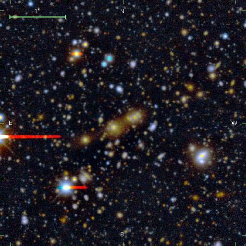
Figure 4: Galaxy cluster coincident with Peak 5 in our high signal-to-noise ratio peak sample. North is up, East is to the left. The cluster candidate contains two bright elliptical galaxies, the eastern-most having a spectroscopic redshift of $z=0.3171$ from the SDSS DR6.

Near the center of our map we detect a new significant lensing peak (Peak 5) with $\nu=4.4$. The optical imaging reveals two brightest cluster galaxies (BCG’s) coincident with this peak, surrounded by an excess of fainter red galaxies (Figure 4). The BCG located at $\rm{R.A.}=09^{\rm{h}}18^{\rm{m}}36^{\rm{s}}.1$, $\rm{decl}=+29^{\circ}53\arcmin 08\arcsec$ has a spectroscopic redshift from the SDSS DR6 of $z=0.3171\pm 0.0002$ (Adelman-McCarthy et al., 2008). We note that the SDSS Maxbcg cluster catalog detects a cluster $\sim 2\arcmin.5$ to the East of this peak with richness $N_{\rm{gals}}=17$ at a slightly lower redshift $z=0.278$, which could also contribute to the lensing signal.

4.3 Low S/N Peaks

We comment here on lower S/N peaks which appear to be associated with the projected structure seen in the lensing reconstruction, but do not fall in our high S/N sample. South of our 5th ranked peak, the $\kappa-\rm{S/N}$ map (Figure 1) reveals a structure which we detect as two peaks; the first located at $\rm{R.A.}=09^{\rm{h}}19^{\rm{m}}26.1^{\rm{s}}$, $\rm{decl.}=+29^{\circ}22\arcmin 06.4\arcsec$ with $\nu=2.7$ and the second located at $\rm{R.A.}=09^{\rm{h}}19^{\rm{m}}19.0^{\rm{s}}$ $\rm{decl.}=+29^{\circ}33\arcmin 04.2\arcsec$ with $\nu=2.4$.

North of Peak 5 we detect another structure in the $\kappa-\rm{S/N}$ map which are resolved as three separate peaks, which we designate as A, B, & C. Peak A is at $\rm{R.A.}=09^{\rm{h}}20^{\rm{m}}56.5^{\rm{s}}$, $\rm{decl.}=+30^{\circ}16\arcmin 36.6\arcsec$ with $\nu=2.7$, Peak B at $\rm{R.A.}=09^{\rm{h}}20^{\rm{m}}55.0^{\rm{s}}$, $\rm{decl.}=+30^{\circ}08\arcmin 44.0\arcsec$ with $\nu=2.7$, and Peak C at $\rm{R.A.}=09^{\rm{h}}20^{\rm{m}}02.9^{\rm{s}}$, $\rm{decl.}=+30^{\circ}06\arcmin 34.6\arcsec$ with $\nu=3.4$. The superpositions of these clusters as well as potentially other clusters along the line of sight likely contribute to the lensing peaks in this structure.

5 Discussion

5.1 False Peak Rate

The noise in weak gravitational lensing reconstructions is influenced by several sources: the distribution in background galaxy positions, ellipticities, and redshifts, spatial variations in the sky background and PSF, and pixel-to-pixel correlations due to the reconstruction methods. As a result, the noise distribution in the lensing maps is strictly non-Gaussian, and there is the potential for “false positives”—peaks in the lensing map that do not correspond to any real objects.

Several previous studies have addressed the issue of the false peak rate in weak lensing mass reconstructions. Hamana et al. (2004) used N-body simulations and ray-tracing to construct catalogs of expected clusters to compare with them. They reported that the completeness and contamination of the catalogs depended on the S/N threshold, and that even at relatively high thresholds ($\sim 5\sigma$), a 20-30% incompleteness and a similar contamination rate would be expected. Schirmer et al. (2007) used a variation of the aperture mass statistic (Schneider, 1996) and estimates of the projected galaxy overdensity to estimate the noise contamination rate in a sample of ESO-WFI fields. When they varied the S/N threshold, they found contamination rates of 30-80%, depending on the depth and seeing of the fields. Hetterscheidt et al. (2005) applied two variations of the aperture mass statistic to 50 deep Very Large Telescope fields; they set their thresholds so as to approximate a 20% contamination rate from noise peaks in their sample. Even though these studies used very different reconstruction methods, data sets and selection criteria, they all concur in finding 20-40% contamination in the rough S/N range that we consider. At lower S/N, the very large number of “detections” in both $\kappa$ and randomized maps indicate a much higher contamination rate. We also mention that Van Waerbeke (2000) studied the noise in weak lensing reconstructions, however their analysis is not directly applicable to us since it does not apply to maximum likelihood reconstructions which use a regularization term.

To estimate the potential false peak rate in our high S/N sample due to lensing shape noise (Kubo et al., 2007) we performed two tests. In our first test we created a mean map of the 100 Monte Carlo reconstructions described in $\S\ref{sec:peaks}$. Each pixel in this map is the average value of this pixel over the individual 100 Monte Carlo map realizations. An average signal-to-noise ratio map is created by dividing this map by the mean of the $\kappa_{\rm{rms}}$ map ($\kappa_{\rm{rms}}/10$) from $\S\ref{sec:peaks}$. Peaks are detected in this average signal-to-noise ratio map using exactly the same procedure used to analyze the original $\kappa-\rm{S/N}$ map. The resulting peak histogram is shown in Figure 5 (Left). We find that above our high signal-to-noise ratio cut ($\nu>3.5$) three peaks are recovered. In a second test we created individual signal-to-noise ratio maps from each of the 100 Monte Carlo realizations. Here each individual Monte Carlo map is divided by the $\kappa_{\rm{rms}}$ map from $\S\ref{sec:peaks}$. Peaks are detected in each of these individual signal-to-noise ratio maps using the same detection procedure described in $\S\ref{sec:peaks}$. The resulting average histogram is shown in Figure 5 (Right). Here we detect $\sim 1$ false peaks above our high S/N cut. Both of the above tests indicate a potential false peak rate due to shape noise of 1-3 (or $\sim 10-25\%$) above our high signal-to-noise ratio cut $(\nu>3.5)$. This percentage compares reasonably well with an estimate based on the proximity of our peaks to overdensities of galaxies in physical and redshift space. Based on the analysis of the environment near the peaks, we see 2-3 (16-25%) of the structures appear not associated with or at $\gtrsim 3\arcmin$ from identified galaxy concentrations.

In the above tests we do not simulate the signal due to uncorrelated large scale structure along the line of sight which will increase the number of detected objects that are falsely interpreted as cluster candidate. The result of these tests therefore are only an estimate to the lower bound of the false peak rate. We emphasize that although false peaks are expected above our high signal-to-noise ratio cut, the majority of our peaks appear to be associated with real clusters which also appear to trace the large-scale filamentary structure.

We note here that residuals in the PSF correction could also potentially cause false peaks. In Kaiser & Squires (1993) type convergence maps this can be probed at some level by creating a B-mode map where source galaxies are rotated by 45 degrees relative to each grid point (e.g. Massey et al. (2007)). One limitation of our maximum likelihood algorithm however is that in its current implementation it cannot create a B-mode map. To probe PSF systematics we have alternatively measured radial shear B-modes for our high significance peaks (Figure 6). In the figure we show profiles for four of these peaks spread over the structures in the F2 field. In each panel the profile is center on the peak coordinates given in Table 1. The measured B-mode for each peak is consistent with zero, indicating that there is no residual contamination coming our PSF correction. Profiles for the other high significance peaks in the field are similarly consistent with a zero B-mode signal.

5.2 Total S/N

To be consistent with previous studies we have selected peaks from the $\kappa-\rm{S/N}$ map as described in $\S\ref{sec:peaks}$. This provides a good method to globally select peaks from the map, however because our reconstruction technique does not track pixel-to-pixel correlations, neither the peak nor the integrated signal-to-noise ratio are good estimates of total signal-to-noise ratio of detection. To calculate the total signal-to-noise ratio for peaks we use a different approach where the original $\kappa$ map and the individual Monte Carlo maps are block averaged at different levels of block size. $\kappa-\rm{S/N}$ maps at each block size are then created in the same manner used to create the original $\kappa-\rm{S/N}$ map $(\S\ref{sec:peaks})$. For small values of block size, due to the pixel-to-pixel correlations in the $\kappa$ and $\kappa_{\rm{rms}}$ maps, both the signal and noise increase linearly, hence the peak signal-to-noise ratio ($\nu$) will stay relatively constant. When the block size becomes larger than the noise correlation length, noise will increase proportional to square root of the block size; therefore, the peak signal-to-noise ratio will grow as more $\kappa$ pixels are used in the average. At some level of block size the peak signal-to-noise ratio will be maximized when the pixel size matches the characteristic size of the cluster. The peak signal-to-noise ratio at this block size can then be used to estimate the total signal-to-noise ratio of detection. Past the maximum as the block size continues to increase we expect that the signal-to-noise ratio will decrease as more noise pixels are added. An example of this technique is shown in Figure 7; here we show peak S/N vs. block size curves for three different peaks in our map. The top curve is for the peak grouping 1 & 2, the middle curve is for peak 5, and the bottom curve is for the peak grouping of 8, 10, & 11. In each of the curves the peak S/N reaches a maximum at certain level of block size, and the value of the peak S/N at that block size is used to approximate the total signal-to-noise ratio of detection. This provides a near-optimal measure of the integrated signal-to-noise ratio for isolated clusters, subject to the constraint of finite pixel sizes. One limitation of our total signal-to-noise ratio estimation is that for large block sizes some peaks can become blended with other peaks. This behavior is exhibited in the top curve (Peaks 1 & 2) and the bottom curve (Peaks 8, 10, & 11). In such cases we can only estimate the total signal-to-noise ratio for the combined system. We list total S/N values using this method for the remaining peaks in Table 1.

Our method of estimating the total signal-to-noise ratio for lensing peaks is qualitatively similar to previously-used techniques in this field. For example, the P-statistics introduced by Schirmer et al. (2007) use variations in the scale of the kernel to effectively identify peaks based on their signal at a smoothing scale matching the peak size, even though they do not take the additional step of identifying the S/N at this kernel with the total S/N of the peak. Our method is also similar to the method used in Kaiser, Squires, & Broadhurst (1995); however in that paper, the method was used to estimate the S/N ratio of faint galaxies rather than in estimating the significance of the lensing signal itself.

5.3 The Abell 781 Complex

As mentioned in $\S\ref{sec:clusters}$ there is a known X-ray cluster associated with the western portion of Abell 781 complex that does not appear in our reconstruction. Our lensing map does hint at a peak at this position but this peak appears to occupy only 1-2 pixels in our map. We recently reported a $1\sigma-2\sigma$ lensing detection of this cluster from an NFW fit in Sehgal et al. (2008). The lensing significance of this cluster is low compared to what is expected from the X-ray mass of this cluster (Sehgal et al., 2008). The low lensing significance could possibly be due to a remaining systematic, or could potentially point toward an interesting physical effect which causes X-ray and lensing masses to be discrepant. Observations of this region with a different telescope/imager are planned, and a detailed analysis will be presented in a future paper.

5.4 A Candidate Void?

In $\S\ref{sec:peaks}$ we mentioned the detection of a candidate underdensity in the $\kappa-{\rm{S/N}}$ map with a significant negative signal-to-noise ratio. Strictly speaking, this region is a relative underdensity since it is underdense relative to other structure in the map. Our ability to detect a relative undersity is unaffected by the mass sheet degeneracy transformation (Schneider & Seitz, 1995). The undersity is located at $\rm{R.A.}=09^{\rm{h}}20^{\rm{m}}22.7^{\rm{s}}$, $\rm{decl.}=+29^{\circ}54\arcmin 03.5\arcsec$ and is detected with a peak significance $\nu\sim 5$ and a total signal-to-noise ratio of $\sim 5.5$. From our lensing reconstruction alone we cannot directly confirm that this underdensity is in fact a void. A galaxy redshift survey, an alternative mapping of structure, is a well known method of directly tracing underdense regions or voids (Geller & Huchra, 1989). We are conducting such a survey in the F2 field, the SHELS redshift survey (Geller et. al., 2005), which should provide additional insights into this underdense region. Confirmation of an underdensity detected in a lensing reconstruction would demonstrate that lensing maps can trace mass underdensities, in addition to overdensities. We note that an excess of negative peaks was reported in Miyazaki et al. (2002), however this excess has not been confirmed with a redshift survey.

6 Summary

In this work we have presented the application of a regularized maximum likelihood weak lensing reconstruction to the Deep Lens Survey F2 field. Our lensing reconstruction reveals several projected structures in the F2 field which appear to lie along a network of potential filaments. In the southwest section of our map we detect a structure which appears to lie at a redshift $z\sim 0.5$. Another structure, the Eastern-most structure in our reconstruction, contains the confirmed cluster Abell 781 and appears to extend southward for over a degree. Known optical clusters at three redshifts $z\sim 0.3,0.43,0.5$ are potentially associated with significant lensing peaks along this structure. Near the center of our map we detect another significant peak at a redshift $z\sim 0.32$. The cluster associated with this lensing peak lies at a roughly the same redshift as many of the peaks in the Eastern structure, however it is unclear if this structure is physically associated with any part of the Eastern structure. These two structures also appear to surround a relative underdense region with $\nu\sim 5$, and total signal-to-noise ratio $\sim 5.5$.

The noise in our reconstruction is estimated from 100 individual Monte Carlo realizations of the source galaxy catalog. We find that generating Monte Carlo $\kappa$ maps with this reconstruction technique is computationally expensive, but does allow us to create a statistically correct $\kappa-\rm{S/N}$ map. Monte Carlo realizations also aid in estimating the number of expected false peaks due to lensing shape noise. We performed two tests here using the Monte Carlo $\kappa$ maps; in one test we created an average Monte Carlo significance map, and in another test we created individual Monte Carlo significance maps and averaged the results. Both of these tests estimate $10-25\%$ false positive detections due to shape noise in our high peak signal-to-noise ratio sample. This is comparable to the number of peaks in our dataset which lack close counterparts in galaxy overdensities.

We have also presented a new method to estimate the total signal-to-noise ratio of detection for lensing peaks. Because pixel-to-pixel correlations are not traced in our lensing reconstruction (or in any traditional direct reconstruction) the peak signal-to-noise ratio underestimates the total lensing significance. Our method of estimating the total lensing significance uses block averaging of the $\kappa$ map and the individual Monte Carlo maps to create $\kappa-\rm{S/N}$ maps with different levels of block size. The peak signal-to-noise ratio will become maximized here when the peak matches the characteristic size of the cluster, and this peak signal-to-noise ratio can be used to estimate the total lensing significance. We find that this method works quite well for isolated peaks, but for a grouping of peaks only the significance of the combined group can be measured.

In future work, photometric redshifts of source galaxies in the F2 field could allow us to make tomographic maps using this method and would also allow for the determination of the mass of significant lensing peaks. Magnification information in the F2 field could also be incorporated into our reconstruction, potentially breaking the mass sheet degeneracy (Broadhurst et al., 1995). We are also pursing optical cluster finding in the DLS, however this is beyond the scope of our current study.

Table 1: Lensing peaks with $\nu>3.5$ in the DLS F2 field

Peak Rank	R.A. (∘)	Decl. (∘)	$\nu$	$z$	$S/N_{t}$
1	140.2294	+30.4677	6.6	0.427, 0.291	7.0
2	140.0829	+30.5070	5.7	0.302	7.0
3	140.3072	+30.2299	5.3	$\sim 0.5$	5.4
4	140.4161	+29.6915	4.5	N/A	4.0
5	139.6471	+29.8726	4.4	0.317	4.9
6	140.2994	+29.5624	4.2	N/A	4.0
7	140.5350	+30.1093	4.1	—	3.6
8	138.9965	+29.5569	3.9	0.53	3.9
9	140.4174	+29.4782	3.9	$\sim 0.34$	4.0
10	139.0007	+29.8431	3.8	0.55	3.9
11	138.9588	+29.6458	3.7	0.53	3.9
12	140.5499	+29.9367	3.6	—	3.6
void	140.0946	+29.9010	$\sim 5$	—	$\sim 5.5$

Note. — Due to the resolution of our map, some peaks are blended together. In this case we report the total signal-to-noise ratio of detection for the combined systems.

Figure 3: Distribution of peak signal-to-noise ratio $(\nu)$ measured from our $\kappa-\rm{S/N}$ map of the DLS F2 field. The solid histogram is the distribution of positive signal-to-noise ratio peaks, the dashed histogram is the distribution of negative signal-to-noise ratio peaks. Negative values have been flipped here to the positive axis.

Figure 5: Distribution of peak signal-to-noise ratio ($\nu$) for the mean Monte Carlo map (Left) and for the average of the individual Monte Carlo maps (Right). As in our real lensing map solid histograms are positive peaks, dashed histograms are negative peaks (where negative values have been flipped to the positive axis). For our high signal-to-noise ratio cut $(\nu>3.5)$ three peaks are recovered in the mean map, $\sim 1$ is recovered in the average of the individual Monte Carlo maps. These tests provide an estimate of the number expected false peaks in our high signal-to-noise ratio sample due to lensing shape noise.

Figure 6: Radial profile of the B-mode component centered on four high-signficance peaks in our convergence map. The B-modes are all consistent with zero signal, indicating that the residuals in the PSF correction are not introducing a spurious signal near each lensing peak.

Figure 7: Examples of total signal-to-noise ratio estimation using the method outlined in $\S\ref{sec:discussion}$. The top curve is for the peak grouping 1 & 2, the middle curve is for peak 5, and the bottom curve is for the peak grouping 8, 10, & 11. In each, the peak signal-to-noise ratio ($\nu$) is measured for different levels of block size after block averaging the $\kappa$ and individual Monte Carlo maps. $\kappa-\rm{S/N}$ maps are then created for each level of block size. The curve for Peak 5, an isolated peak in our map, exhibits a clear maximum. For the two other curves the maximum is not as well defined due to the proximity of nearby peaks, however an estimate for each peak grouping can still be obtained. As expected the total signal-to-noise ratio values are higher than our estimates using only the peak signal-to-noise ratio from our $\kappa-\rm{S/N}$ map.

References

- Adelman-McCarthy et al. (2008) Adelman-McCarthy, J.K., et al., 2008, ApJS, 175, 297
- Bartelmann et al. (1996) Bartelmann, M., Narayan, R., Seitz, S., Schneider, P., 1996, ApJ, 464, L115
- Beckwith et al. (2006) Beckwith, S., et al., 2006, AJ, 132, 1729
- Bertin & Arnouts (1996) Bertin, E. & Arnouts, S., 1996, A&AS, 117, 393
- Bernstein & Jarvis (2002) Bernstein, G.M., Jarvis, M. 2002, AJ, 123, 583B
- Bradac et al. (2006) Bradac, M., 2006, ApJ, 652, 937B
- Bridle et al. (1998) Bridle, S.L, Hobson, M.P., Lasenby, A.N., & Saunders, R. 1998, MNRAS, 299, 895
- Broadhurst et al. (1995) Broadhurst, T.J., Taylor, A. & Peacock, J. 1995, ApJ, 438, 49
- Carlstrom et. al. (2002) Carlstrom, J.E., Holder, G.P., & Reese, E.D. 2002, ARA&A, 40, 643
- Fischer & Tyson (1997) Fischer, P., Tyson, A.J. 1997, AJ, 114, 14F
- Gavazzi & Soucail (2007) Gavazzi, R., Soucail, G., 2007, A&A, 462
- Geller & Huchra (1989) Geller, M.J., Huchra, J.P., 1989, Sci, 246, 897
- Geller et. al. (2005) Geller, M.J., Dell’Antonio, I.P., Kurtz, M.J., Ramella, M., Fabricant, D.G., Caldwell, N., Tyson, J.A., Wittman, D. 2005, ApJ, 635, L125
- Haiman et al. (2001) Haiman, Z., Mohr, J.J., Holder, G.P., 2001, ApJ, 553, 545
- Hamana et al. (2004) Hamana, T., Takada, M., & Yoshida, N. 2004, MNRAS, 350, 893
- Hennawi & Spergel (2005) Hennawi, J., & Spergel, D. 2005, ApJ, 624, 59
- Hetterscheidt et al. (2005) Hetterscheidt, M., Erben, T., Schneider, P., Maoli, R., van Waerbeke, L., & Mellier, Y., 2005, A&A, 442, 43
- Heymans (2006) Heymans, C., et al., 2006, MNRAS, 368, 1323
- Hirata & Seljak (2003) Hirata, C., & Seljak, U., 2003, MNRAS, 343, 459
- Jain & Van Waerbeke (2000) Jain, B., & Van Waerbeke, L., 2000, ApJ, 530, L1
- Jee et al. (2007) Jee, M.J., et al., 2007, ApJ, 661, 728
- Kaiser & Squires (1993) Kaiser, N. & Squires, G. 1993, ApJ, 404, 441
- Kaiser, Squires, & Broadhurst (1995) Kaiser, N., Squires, G., & Broadhurst, T. 1995, ApJ, 449, 460
- Khiabanian & Dell’Antonio (2008) Khiabanian, H. & Dell’Antonio, I.P. 2008, ApJ, 684, 794
- Kochanek et al. (2005) Kochanek, C.S., Schneider, P., Wambsganss, J., Gravitational Lensing: Strong, Weak, & Micro. Lecture Notes of the 33rd Saas-Fee Advanced Course, G. Meylan & P. North (eds.), Springer-Verlag:Berlin
- Koester et al. (2007) Koester, B., et al. 2007, ApJ, 660, 221
- Kubo et al. (2007) Kubo, J.M., Stebbins, A., Annis, J., Dell’Antonio, I.P., Lin, H., Khiabanian, H., & Frieman, J. 2007, ApJ, 671, 1466
- Lucy (1994) Lucy, 1997, A&A, 289, 983
- Marian & Bernstein (2006) Marian, L., & Bernstein, G.M. 2006, PhRvD, 7313525
- Massey et al. (2007) Massey, R., et al. 2007, Nature, 445, 286M
- Miyazaki et al. (2002) Miyazaki, S., et al. 2002, ApJ, 580, L97
- Miyazaki et al. (2007) Miyazaki, S., Hamana, T., Ellis, R.S., Kashikawa, N., Massey, R.J., Taylor, J., Refregier, A. 2007, ApJ, 669, 714
- Muller et al. (1998) Muller G., Reed R., Armandroff T., Boroson T., Jacoby G., 1998, in D Odorico S., ed., Proc. SPIE Vol. 3355, Optical Astronomical Instrumentation. SPIE, Bellingham, p. 577
- Navarro et al. (1996) Navarro, J.F., Frenk, C.S., & White, S.D. 1996, ApJ, 462, 563
- Oyaizu et al. (2008) Oyaizu, H., Lima, M., Cunha, C., Lin, H., Frieman, J., Sheldon, E.S., 2008, ApJ, 674, 768
- Press et al. (1992) Press, W.H., Teukolsky, S.A., Vetterling, W.T., & Flannery, B.P., 1992, Numerical Recipies in C, Cambridge (Cambridge University Press)
- Rosati et al. (2002) Rosati, P., Borgani, S., & Norman, C. 2002, ARA&A, 40, 539
- Schirmer et al. (2007) Schirmer, M., Erben, T., Hetterscheidt, M., & Schneider, P. 2007, A&A, 462, 9875
- Schneider & Seitz (1995) Schneider, P. & Seitz, C. 1995, A&A, 294, 411
- Schneider (1996) Schneider, P., 1996, MNRAS, 283, 837
- Schneider et al. (2000) Schneider, P., King L., Erben, T., 2000, MNRAS, 353, 41
- Sehgal et al. (2008) Sehgal, N., Hughes, J.P., Wittman, D., Margoniner, V., Tyson, A.J., Gee, P., Dell’Antonio, I.P., 2008, ApJ, 673, 163
- Seitz et al. (1998) Seitz, S., Schneider, P., Bartelmann, M. 1998, A&A, 337, 325
- Smith et al. (2001) Smith, D.R., Bernstein, G.M., Fischer, P., Jarvis, M., 2001, ApJ, 551, 643
- Tyson (2002) Tyson, J.A., 2002, SPIE, 4836, 10
- Van Waerbeke (2000) Van Waerbeke, L. 2000, MNRAS, 313, 524
- White et al. (2002) White, M., van Waerbeke, L., & Mackey, J. 2002, ApJ, 575, 640
- Wittman et al. (2000) Wittman, D.M., Tyson, J.A., Kirkman, D., Dell’Antonio, I.P., Bernstein, G. 2000, Nature, 405, 143
- Wittman et al. (2002) Wittman, D., et al. 2002, SPIE, 4836, 73W
- Wittman et al. (2006) Wittman, D., Dell’Antonio, I.P., Hughes, J.P., Margoniner, V.E., Tyson, A.J., Cohen, J.G., Norman 2006, ApJ, 643, 128