Distortion of the perfect lattice structure in bilayer graphene

Abstract

We consider the instability of bilayer graphene with respect to a distorted configuration in the same spirit as the model introduced by Su, Schrieffer and Heeger. By computing the total energy of a distorted bilayer, we conclude that the ground state of the system favors a finite distortion. We explore how the equilibrium configuration changes with carrier density and an applied potential difference between the two layers.

I Introduction

A planar arrangement of carbon atoms covalently bound via $sp^{2}$ orbitals exhibits a honeycomb structure and is denoted graphene. Graphene rose rapidly to the forefront of research in condensed matter physics, mostly because of the peculiar electronic structure that emerges from its crystal structure, and the consequent wealth of rich and unexpected phenomenaCastro Neto et al. (2007). Seminal experiments on two dimensional crystals established graphene as an accessible realityNovoselov et al. (2004), and immediately unveiled numerous surprises, both on a fundamental level – like a new form of quantized Hall effect – and on a practical and technological level – like the highly efficient field effect and high electronic mobility Novoselov et al. (2005a, b). Most of the appealing phenomenology of graphene owes to the fact that electron dynamics in this system can be described in terms of chiral massless Dirac fermionsNovoselov et al. (2005a) and, in fact, graphene does exhibit many properties characteristic of relativistic particlesCastro Neto et al. (2006); Katsnelson and Novoselov (2007).

Equally remarkable phenomena occur in bilayer graphene, which consists of two adjacent graphene planes stacked in the A-B fashion typical of graphite. Bilayer graphene displays the same sample quality and quasi-ballistic transport characteristic of its single layer counterpartMorozov et al. (2008), but brings also its share of new physics stemming from the nature of its charge carriers: chiral massive electronsNovoselov et al. (2006). Most interesting is the fact that, although gapless in its pristine form, a potential difference between the two layers opens a gap in the spectrum that can be controlled via chemical dopingOhta et al. (2006) or gatingMcCann (2006); Castro et al. (2007); Oostinga et al. (2008).

Despite such favorable prospects, the amount of knowledge gathered in the context of bilayer graphene still lags behind the intensity committed to single layer graphene. In this brief paper, we address a particular aspect of the electron-phonon interaction in bilayer graphene, namely the tendency to relax the perfect crystal structure and generate a static, uniform deformation. This effect is inspired, and similar in spirit, to the well known Peierls instability that occurs in polyacetylene chains. As shown by Su, Schrieffer and Heeger (SSH)Su et al. (1979, 1980), in polyacetylene the one dimensional chain of carbon atoms has a half-filled electronic ground state that is unstable with respect to a spontaneous dimerization. This dimerization opens a sizeable gap in the spectrum that can be easily detected experimentallyFincher et al. (1978).

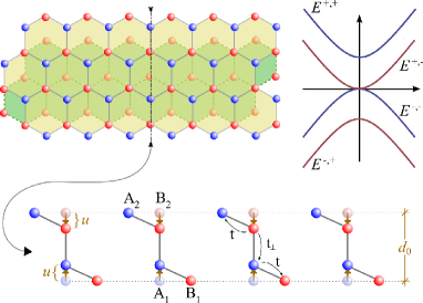
Figure 1: (color online) Transverse view (bottom) along the dashed-dotted line (top left) of the lattice distortion considered in the text. The vertical displacement of the carbon atoms connected by the hopping integral $t_{\perp}$ is represented by the parameter $u$. In the top right we schematically represent the bandstructure in the vicinity of the Dirac point.

The instability we envisage for bilayer graphene is related with the application of SSH’s ansatz to the interplane hopping, $t_{\perp}$. From the outset, the atoms lying in the A and B sublattices within each layer are not equivalent, since only one of the sublattices connects to the adjacent plane (Fig. 1). This has important experimental consequences: one example is the known fact that in tunneling experiments one typically detects only one of the sublattices of the topmost layerRutter et al. (2007). In the absence of a potential difference between the two layers (unbiased situation), the bilayer is a zero gap semiconductor, with hyperbolic bands touching at the Fermi energy. A change in the interlayer hopping will not change this situation, and thus the gap can still be tuned through the potential difference between layers. However, as shown below, the electron-phonon interaction might indeed lead to a stable distorted configuration.

II The model

II.1 Tight binding description of a biased bilayer

The electronic Hamiltonian of a biased bilayer consists of two contributions, $H_{e}=H_{tb}+H_{V}$, where $H_{tb}$ is the tight-binding Hamiltonian for the graphene bilayer, and $H_{V}$ reflects the electrostatic bias applied between the two graphene planes. The tight-binding Hamiltonian $H_{tb}$ contains in itself three terms describing electron itinerancy among each individual plane and between the two planes. In detail we have

$$H_{tb}=H_{tb1}+H_{tb2}+H_{\perp}\,,$$ (1)

with

$$H_{tb1}= - t\sum_{\mathbf{R},\sigma}[a^{\dagger}_{1\sigma}(\mathbf{R})b_{1\sigma}(\mathbf{R})+a^{\dagger}_{1\sigma}(\mathbf{R})b_{1\sigma}(\mathbf{R}-\mathbf{a}_{1})$$ (2)

$$+ a^{\dagger}_{1\sigma}(\mathbf{R})b_{1\sigma}(\mathbf{R}-\mathbf{a}_{2})+\text{H.c.}]\,,$$

$$H_{tb2}= - t\sum_{\mathbf{R},\sigma}[a^{\dagger}_{2\sigma}(\mathbf{R})b_{2\sigma}(\mathbf{R})+a^{\dagger}_{2\sigma}(\mathbf{R}+\mathbf{a}_{1})b_{2\sigma}(\mathbf{R})$$ (3)

$$+ a^{\dagger}_{2\sigma}(\mathbf{R}+\mathbf{a}_{2})b_{2\sigma}(\mathbf{R})+\text{H.c.}]\,,$$

$$H_{\perp}=-t_{\perp}\sum_{\mathbf{R},\sigma}[a^{\dagger}_{1\sigma}(\mathbf{R})b_{2\sigma}(\mathbf{R})+b^{\dagger}_{2\sigma}(\mathbf{R})a_{1\sigma}(\mathbf{R})]\,,$$ (4)

and

$$H_{V}= \frac{V}{2}\sum_{\mathbf{R},\sigma}[a^{\dagger}_{1\sigma}(\mathbf{R})a_{1\sigma}(\mathbf{R})+b^{\dagger}_{1\sigma}(\mathbf{R})b_{1\sigma}(\mathbf{R})]$$ (5)

$$- \frac{V}{2}\sum_{\mathbf{R},\sigma}[a^{\dagger}_{2\sigma}(\mathbf{R})a_{2\sigma}(\mathbf{R})+b^{\dagger}_{2\sigma}(\mathbf{R})b_{2\sigma}(\mathbf{R})]\,.$$

In the above equations $\mathbf{a}_{1}$ and $\mathbf{a}_{2}$ represent the elementary translations of the honeycomb lattice. In the presence of an electrostatic bias $V$, the electronic dispersion is given by the four branches

$$E^{\pm,\pm}_{\mathbf{k}}=\pm\frac{1}{2}\sqrt{2t^{2}_{\perp}+V^{2}+4t^{2}|\phi_{\mathbf{k}}|^{2}\pm\Delta_{\mathbf{k}}}\,,$$ (6)

where

$$\Delta_{\mathbf{k}}=2\sqrt{t^{4}_{\perp}+4t^{2}(t^{2}_{\perp}+V^{2})|\phi_{\mathbf{k}}|^{2}}\,.$$ (7)

When $V=0$ Eq. (6) simplifies to

$$E^{\pm,\pm}_{\mathbf{k}}=\pm\frac{1}{2}\Bigl{(}\pm\,t_{\perp}+\sqrt{t^{2}_{\perp}+4t^{2}|\phi_{\mathbf{k}}|^{2}}\Bigr{)}\,,$$ (8)

where $\phi_{\mathbf{k}}$ is associated with the dispersion of a single layer, and is given by

$$\phi_{\mathbf{k}}=1+e^{i\mathbf{k}\cdot\mathbf{a}_{1}}+e^{i\mathbf{k}\cdot\mathbf{a}_{2}}\,.$$ (9)

In order to proceed analytically, we approximate $|\phi_{\mathbf{k}}|$ by

$$|\phi_{\mathbf{k}}|\simeq\frac{3}{2}aq\,,$$ (10)

where we took $\mathbf{k}=\mathbf{K}+\mathbf{q}$ to be close to the Dirac point in the honeycomb Brillouin zone, and amounts to using the effective mass approximation for bilayer graphene ($a$ is the carbon-carbon distance).

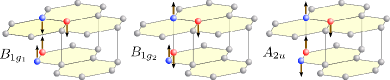
Figure 2: (color online) Phonon modes along the $c$-axis in graphite, using the notation of LABEL:~Dresselhaus and Dresselhaus, 2002. The modes $A_{2u}$ and $B_{1g_{2}}$ are nearly degenerate at the center of the Brillouin zone, with $\omega\simeq 870\,\text{cm}^{-1}$ Dresselhaus and Dresselhaus (2002); Wirtz and Rubio (2004).

II.2 Parametrization of Distortion

We consider a distortion of the perfect lattice structure of the bilayer, such that the $A$ and the $B$ atoms, connected by the hoping parameter $t_{\perp}$, distort along the vertical direction by an amount $u_{i}$ (Fig. 1). In the spirit of the SSH model for polyacetyleneSu et al. (1980) we assume that, to leading order in the strain, the effect of this distortion is to change the value of $t_{\perp}$ according to

$$t_{\perp}=t^{0}_{\perp}(1+\alpha u_{i})\,,$$ (11)

where $t^{0}_{\perp}$ is the value of the interlayer hoping of the undistorted lattice. For small $u_{i}$, the in-plane hopping $t$ is affected by this distortion only at higher orders in $u_{i}$, and therefore we neglect its variation. This distortion will naturally induce an elastic restoring force that we parametrize through the term

$$H_{el}=K\sum_{i=1}^{N_{c}}u^{2}_{i}+\sum_{i=1}^{N_{c}}\frac{P^{2}_{i}}{M}\,,$$ (12)

$N_{c}$ denoting the number of unit cells. In the static and homogeneous situation the kinetic term gives an average null contribution and all $u_{i}$ acquire the same mean value: $u_{i}=u$. This leads to a total elastic energy that reads:

$$E_{\text{el}}=K\sum_{i=1}^{N_{c}}u^{2}=N_{c}u^{2}\,.$$ (13)

The stability analysis of such a distorted phase proceeds by minimization of the total electronic and elastic energy, given by $H_{e}+H_{el}$, with respect to the distortion $u$. We underline that, unlike in the original polyacetylene modelSu et al. (1980), the parametrization (11) does not change the original periodicity of the lattice, and therefore does not require a density commensurability.

II.3 Estimation of parameters

A precise estimation of the parameters required for the computation of the stable distorted configuration is not easy nor unique. On the one hand, little is know with respect to the structural and elastic properties of a graphene bilayer, and thus we will rely on the corresponding knowledge that exists for graphite. On the other hand, details like the type of substrate, can significantly alter these parameters, as happens, for instance with the phonon spectrum that can be sensitive to substrate and other constraints in the system.

We will therefore resort to the structural parameters (lattice constant and elastic coefficients) known for A-B stacked graphite. The carbon-carbon distance is $a\simeq 1.42$ Å, and the graphene unit cell has an area given by $A_{c}=3\sqrt{3}a^{2}/2$. The equilibrium interlayer distance is given by $d_{0}=c_{0}/2\simeq 3.35$ Å, and corresponds to half the unit cell height of A-B stacked graphiteJansen and Freeman (1987); Boettger (1997); Mounet and Marzari (2005).

The value of the stiffness, $K$, can be estimated from the phonon spectrum of graphite. In particular the $B_{1g_{2}}$ optical (out-of-plane) phonon mode has a frequency of $\omega\approx 870\,\text{cm}^{-1}$, which is seen both experimentallyNemanich et al. (1977), and from ab-initio calculations Wirtz and Rubio (2004). As a result of the week interlayer interaction, this phonon is essentially degenerate with the out-of-plane phonon $A_{2u}$ present in a single layer of graphene. These normal modes are represented in Fig. 2. We can assume that $K$ relates to this frequency through $Ka^{2}\sim m\omega^{2}a^{2}/4$, where $m$ is the carbon atom mass, and $a\simeq 1.42$ Å is the carbon-carbon distanceFuchs and Lederer (2007). As a result we obtain as estimate for the stiffness $K\simeq 8.5\,\text{eV.\AA}^{-2}$.

With respect to the electron-phonon coupling $\alpha$, its estimation is most straightforward from the knowledge of how the interplane hopping varies with distance. The interplane hopping, $t_{\perp}$ corresponds to the tight-binding parameter $V_{pp\sigma}$ in the two center Slater-Koster formalismSlater and Koster (1954); Harrison (1999). For instance, assuming that

$$V_{pp\sigma}(r)\simeq Ae^{-\alpha r}$$ (14)

one can extract $\alpha$ from interpolation of the hoppings $\gamma_{1}$ the in-plane $V_{pp\sigma}(a)$ for graphite. Using the valuesDresselhaus and Dresselhaus (2002); Kim and Castro Neto (2007) $\gamma_{1}\approx 0.4~{}\text{eV}$ and $V_{pp\sigma}(a)\approx 3.7~{}\text{eV}$ we obtain $\alpha\approx 1.2~{}\text{\AA}^{-1}$. Alternatively to the formula (14), one could use a more refined interpolation formula for $V_{pp\sigma}(r)$ as discussed in LABEL:~Papaconstantopoulos et al., 1998. This yields $\alpha\approx 1.8~{}\text{\AA}^{-1}$, consistent with the previous estimate.

Finally, several recent experiments on the bilayerOhta et al. (2007); Malard et al. (2007); Yan et al. (2007) show that the value of $t_{\perp}^{0}$ is essentially the value expected in graphite, $t_{\perp}^{0}\approx 0.3~{}\text{eV}$, the same applying to the in-plane hopping, $t\approx 3~{}\text{eV}$.

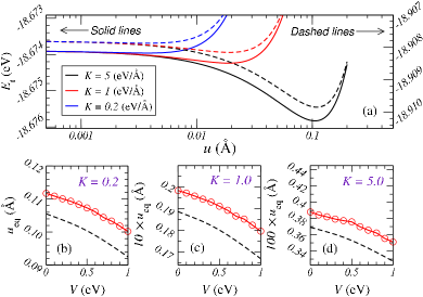
Figure 3: (color online) (a) Total energy E_t per unit cell as a function of the deformation parameter $u$, and for different values of $K$. The left (right) vertical axis pertains to the solid (dashed) curves. (b-d) The equilibrium radius as a function of the bias voltage, $V$. In all panels dashed lines refer to the Dirac approximation, whereas full lines have been calculated using the full tight-binding dispersion in Eq. (6). Notice that in panels (c) and (d) the vertical axis is amplified 10 and 100 times, respectively. Other parameters used are $t^{0}_{\perp}=0.3$ eV, $t=3.0$ eV, $\alpha=1.5$Å^-1.

III Ab-initio calculation of the elastic constant

In addition to the above estimates of the model parameters, we have extracted the compression elastic constant from a first principles calculation. Density functional calculations in graphite and related compounds must be carried with caution for it is known that different implementations of density functional theory can yield noticeably different results Wirtz and Rubio (2004); Lazzeri et al. (2008). Having this in mind, we calculated the equilibrium distance between graphene planes in the bilayer by resorting to two different approximations: the Generalized Gradient Approximation (GGA) and the Local Density Approximation (LDA).

GGA — We sampled the BZ according to the scheme proposed by Monkhorst-Pack Monkhorst and Pack (1968), with a grid of $12\times 12\times 4$ $\mathbf{k}$-points. Bilayer graphene was modeled in a slab geometry by including a vacuum region in a supercell containing 4 carbon atoms (2 for each graphene sheet). In the normal direction ($z$-direction), the vacuum separating repeating slabs has more than 10 Å, and the size of the supercell in the $z$-direction was optimized to make sure there was no interaction between repeating slabs.

LDA — In this case the BZ was sampled within the same scheme with a grid of $4\times 4\times 1$ $\mathbf{k}$-points, and using a supercell comprising 8 carbon atoms (4 for each sheet). Adjacent slabs along the $z$ direction were separated by more than 30 Å, and the size of the supercell along this direction was again optimized.

In either case an increase in the number of sampling points did not result in a significant total energy change, and the vertical separation quoted above guarantees the absence of interaction between adjacent slabs. We used dual-space separable pseudopotentials by Hartwigsen, Goedecker, and HutterHartwigsen et al. (1998) to describe the ion cores. In a first step, all the atoms were fully relaxed to their equilibrium positions. Then one of the graphene sheets was moved as a whole in the $z$-direction by very small displacements, and the total energy of the system was calculated, without any further relaxation.

Figure 4 shows the GGA variation of the total energy relative to the relaxed sample, as a function of the displacement from the equilibrium position. Also shown is the parabola that was fitted to the calculated values. The fitting gave a value of $K=0.615\pm 0.002$ eV/Ų, per unit cell. The same calculation within LDA yields $K=4.15\pm 0.06$ eV/Ų. The two calculations therefore differ by one order of magnitude, signaling the fact that, like other systems derived from graphite, density functional calculations are very sensitive to the details of the approximation used.

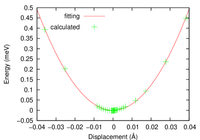
Figure 4: Energy as a function of distance between layers measured with respect to the equilibrium position, and calculated within the GGA. The positive direction indicates a displacement towards the other graphene sheet. The zero value energy is the energy of the fully relaxed sample.

IV Total energy at Constant $\mu$

Our main objective is to quantify the equilibrium distortion that is expected to emerge from the competition between elastic and electronic energies in the ground state. For illustration purposes we consider first the computation of the total energy in the (potentially artificial) case where the chemical potential is held constant. In particular, we assume that the density of carriers in the bilayer is such that the chemical potential is located between $E^{+,+}_{q=0}$ and $E^{+,-}_{q=0}$:

$$\mu=\frac{V+\sqrt{V^{2}+4t_{\perp}^{2}}}{4}\,.$$ (15)

Let us start with an unbiased bilayer ($V=0$). In this case the total electronic energy per unit cell is given by

$$\frac{E_{e}}{N_{c}}=\frac{gA_{c}}{2\pi}\int^{q_{c}}_{0}qdq\bigl{(}E_{q}^{-,+}+E_{q}^{-,-}\bigr{)}+\frac{gA_{c}}{2\pi}\int^{q_{F}}_{0}qdqE_{q}^{+,-}\,.$$ (16)

The integral is elementary leading to

$$\frac{E_{e}}{N_{c}} =\frac{gA_{c}}{2\pi}\,t_{\perp}\biggl{(}\frac{q_{t}^{2}}{6}-\frac{q_{F}^{2}}{4}\biggr{)}-\frac{gA_{c}}{6\pi}\,t_{\perp}q_{t}^{2}\biggl{[}1+\biggl{(}\frac{q_{c}}{q_{t}}\biggr{)}^{2}\biggr{]}^{3/2}$$

$$+\frac{gA_{c}}{12\pi}\,t_{\perp}q_{t}^{2}\biggl{[}1+\biggl{(}\frac{q_{F}}{q_{t}}\biggr{)}^{2}\biggr{]}^{3/2}\,,$$ (17)

where the momenta $q_{F}$, $q_{c}$ and $q_{t}$ are defined as

$$q_{t}=\frac{t_{\perp}}{3ta}\,,\;q_{c}=\sqrt{\frac{2\pi}{A_{c}}}\,,\;q_{F}=\frac{\sqrt{(2\mu+t_{\perp})^{2}-t_{\perp}^{2}}}{3ta}\,,$$ (18)

and $A_{c}=3\sqrt{3}a^{2}/2$ is the area of the graphene unit cell. The total energy $E_{t}$ per unit cell is given by

$$\frac{E_{t}}{N_{c}}=\frac{E_{e}}{N_{c}}+Ku^{2}\,.$$ (19)

These two terms compete in such a way that the minimum energy state is achieved for a finite value of $u$.

The dashed lines of the top panels of Fig. 3 represent the total energy, $E_{t}$, as a function of the deformation $u$, using different values of the stiffness parameter, $K$. It is also instructive to investigate to what extent the approximation (10) influences the equilibrium deformations and, for that, we have performed the calculation of the total energies using the full tight-binding dispersions of Eq. (6). The results so obtained are represented in the same figure by the solid lines. It is clear from Fig. 3(a), that, besides yielding larger slightly larger absolute values for the energy, the full dispersion increases the equilibrium deformation by about 5 to 10%.

The analytical calculation in the presence of a finite bias ($V\neq 0$), is also straightforward. The total energy is still given by Eq. (16), where $E_{\mathbf{k}}^{\pm,\pm}$ is now given by (6). The energy integrals are given in the appendix, the final result being

$$\frac{E_{\text{el}}}{N_{c}}=\frac{gA_{c}}{2\pi}\biggl{[}F^{-,+}(k)\Bigr{|}_{0}^{q_{c}}+F^{-,-}(k)\Bigr{|}_{0}^{q_{c}}+F^{+,-}(k)\Bigr{|}_{0}^{q_{F}}\biggr{]}\,.$$ (20)

The primitives $F^{\eta_{1},\eta_{2}}(k)$ are calculated in the appendix, with the final result

$$F^{\eta_{1},\eta_{2}}(k) =\frac{\eta_{1}}{8\nu_{F}^{2}(t_{\perp}^{2}+V^{2})}\biggl{\{}\frac{R^{3/2}}{3\gamma}-\frac{\gamma x+\eta_{2}}{2\gamma^{2}}\eta_{2}\sqrt{R}$$

$$-\frac{\eta_{2}\Delta}{8\gamma^{5/2}}\log\bigl{(}2\sqrt{\gamma R}+2\gamma x+2\eta_{2}\bigr{)}\biggr{\}}\,,$$ (21)

and the remaining parameters are defined in (36).

Placing the chemical potential again at the midpoint between the two conduction bands at $q=0$,

$$\mu=(V+\sqrt{4t^{2}_{\perp}+V^{2}})/4\,,$$ (22)

the corresponding Fermi wavevector is

$$q_{F}=\frac{1}{2\nu_{F}}\sqrt{V^{2}+4\mu+2\sqrt{4\mu(t_{\perp}^{2}+V^{2})-t_{\perp}^{2}V^{2}}}\,,$$ (23)

and we obtain the results shown in the lower panel of Fig. 3 for the equilibrium radius. When $V$ varies between 0 and 1 eV, the equilibrium radius shows a relative variation of $\sim 15\%$. In addition, it can be seen that the difference between using the Dirac approximation and the full tight-binding dispersion is, in accordance with the above, essentially a systematic increase in the equilibrium radius. For this reason, henceforth we will restrict the discussion to the results obtained within the Dirac approximation.

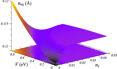
Figure 5: (color online) Equilibrium deformation, $u_{\text{eq}}$, as a function of the electron density per unit cell ($n_{e}$) and the bias voltage ($V$). The parameters used are $t^{0}_{\perp}=0.3~{}\text{eV}$, $t=3.0~{}\text{eV}$, $K=0.2~{}\text{eV.\AA}^{-2}$ and $\alpha=1.5~{}\text{\AA}^{-1}$.

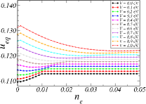
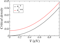
Figure 6: (color online) 6 Selected cuts from Fig. 5 at constant bias $V$. For clarity, successive curves have been shifted vertically by 0.001 in the order of increasing $V$. 6 The densities $n_{e}^{*}$ and $n_{e}^{**}$ defined in Eq. (24), plotted as a function of $V$ for the same parameters used in Fig. 5.

V Total Energy at Constant $\mathbf{n_{e}}$

We consider now the more relevant case of a bilayer with constant carrier density, which can be tuned, for instance, through a gate voltage. We define $n_{e}$ as the number of electrons per unit cell, with respect to the charge-neutral situation in which the valence bands are fully occupied. In addition we will be concerned with electron doping only. The calculation of the electronic energy in this case requires, in general, the consideration of three distinct possibilities. Assuming a biased situation, and with respect to the notation defined in Fig. 7, we can have:

1. the Fermi level lying between $E_{1}$ and $E_{2}$, in which case the Fermi surface consists of a Fermi ring characterized by two Fermi momenta $q_{F}^{III,1}$ and $q_{F}^{III,2}$, and the phase space exhibits a central hollow;

2. the Fermi level lying between $E_{2}$ and $E_{3}$, where we have a more conventional Fermi surface;

3. the Fermi level lying above the bottom of the uppermost band, in which case we have again two Fermi momenta, $q_{F}^{III}$ and $q_{F}^{IV}$, but the phase space is now simply connected.

The boundaries of these regimes can be easily identified through the two threshold densities

$$n_{e}^{*}=\frac{gA_{c}}{4\pi}\,q_{2}^{2}\,,\quad\text{and}\quad n_{e}^{**}=\frac{gA_{c}}{4\pi}\,q_{3}^{2}\,.$$ (24)

It follows that the total electronic energy is computed as

$$\frac{E_{e}}{N_{c}} =\frac{gA_{c}}{2\pi}\int^{q_{c}}_{0}qdq\bigl{(}E_{q}^{-,+}+E_{q}^{-,-}\bigr{)}$$ (25)

$$+\frac{gA_{c}}{2\pi}\int^{q_{F}^{III,2}}_{q_{F}^{III,1}}qdqE_{q}^{+,-}+\frac{gA_{c}}{2\pi}\int^{q_{F}^{IV}}_{0}qdqE_{q}^{+,+}\,,$$

where the integration limits of the last two terms are given by (see also Fig. 7 for notation)

$$n_{e}<n_{e}^{*}:$$ (26a)

$$q_{F}^{IV}=0\,,$$

$$\begin{cases}n_{e}=\frac{gA_{c}}{4\pi}\biggl{(}\Bigl{(}q_{F}^{III,2}\Bigr{)}^{2}-\Bigl{(}q_{F}^{III,1}\Bigr{)}^{2}\biggr{)}\\ 2\nu_{F}^{2}\Bigl{(}q_{F}^{III,1}\Bigr{)}^{2}-\sqrt{t_{\perp}^{4}+4\nu_{F}^{2}\Bigl{(}q_{F}^{III,1}\Bigr{)}^{2}\bigl{(}t_{\perp}^{2}+V^{2}\bigr{)}}=2\nu_{F}^{2}\Bigl{(}q_{F}^{III,2}\Bigr{)}^{2}-\sqrt{t_{\perp}^{4}+4\nu_{F}^{2}\Bigl{(}q_{F}^{III,2}\Bigr{)}^{2}\bigl{(}t_{\perp}^{2}+V^{2}\bigr{)}}\end{cases}$$

$$n_{e}^{*}<n_{e}<n_{e}^{**}:$$ (26b)

$$q_{F}^{IV}=0\,,$$

$$q_{F}^{III,1}=0\,,$$

$$q_{F}^{III,2}=\frac{gA_{c}}{4\pi}\biggl{(}\frac{1}{n_{e}}\biggr{)}^{-1/2}\,.$$

$$n_{e}>n_{e}^{**}:$$ (26c)

$$q_{F}^{III,1}=0\,,$$

$$\begin{cases}n_{e}=\frac{gA_{c}}{4\pi}\biggl{(}\Bigl{(}q_{F}^{III,2}\Bigr{)}^{2}+\Bigl{(}q_{F}^{IV}\Bigr{)}^{2}\biggr{)}\\ 2\nu_{F}^{2}\Bigl{(}q_{F}^{III,2}\Bigr{)}^{2}+\sqrt{t_{\perp}^{4}+4\nu_{F}^{2}\Bigl{(}q_{F}^{III,2}\Bigr{)}^{2}\bigl{(}t_{\perp}^{2}+V^{2}\bigr{)}}=2\nu_{F}^{2}\Bigl{(}q_{F}^{IV}\Bigr{)}^{2}-\sqrt{t_{\perp}^{4}+4\nu_{F}^{2}\Bigl{(}q_{F}^{IV}\Bigr{)}^{2}\bigl{(}t_{\perp}^{2}+V^{2}\bigr{)}}\end{cases}$$

Minimizing the total energy with respect to $u$ yields the equilibrium displacements plotted in Fig. 5, for different electron densities and bias voltages. The typical deformations for the parameters quoted in the figure are $\sim 0.11~{}\text{\AA}$, which represents $\sim 8$% of the carbon-carbon distance, $a$. The variation of $u_{\text{eq}}$ with $n_{e}$ and $V$ is non-monotonic. In particular, one notices that, for constant $V$, the equilibrium deformation tends to saturate beyond a given density. This can be appreciated in more detail in Fig. 6, where we present selected cuts of the same surface. The saturation can be understood from the interplay of two factors: on the one hand, the variation of $V$ and $n_{e}$ induce changes in the bandstructure only in a region close to the neutrality point; on the other hand, for high enough density, the Fermi level will always be considerably above the bottom of the uppermost band ($E_{3}$ in Fig. 7). In fact, comparing the values of $n_{e}^{*}$ and $n_{e}^{**}$ presented in Fig. 6, one can verify that the first sets the scale for the minimum in the curves of $u_{\text{eq}}$ versus $n_{s}$, therefore defining the shape of the valley in the plot of Fig. 5. The value $n_{e}^{**}$, on the other hand, marks the onset of saturation.

VI Discussion and Conclusions

We have shown that a graphene bilayer with A-B stacking can be unstable with respect to a Peierls-like distortion affecting the interplane bonds. This distortion preserves the bandstructure of the system, in the sense that, unlike the original Peierls problem, it does not lead to a gap in the unbiased case, nor to its closing in the biased situation. In addition, it was found that the general effect of the bias voltage is to increase the equilibrium deformation.

By comparing the results obtained with the full tight-binding dispersion of bilayer graphene with the effective mass approximation [Fig. 3(c-e)], we concluded that the former does not introduce significant changes in the equilibrium results, and therefore the low energy approximation is adequate to study this instability.

For the values of $K$ used in Fig. 5, the magnitude of the deformation corresponds to roughly $10$% of the in-plane carbon-carbon distance, and is significant. However, at this point one can hardly be definite about a specific value of the equilibrium deformation on account of the uncertainties in the estimation of the parameters $K$ and $\alpha$. The value used for $K$ is close to the compressive stiffness found with the GGA calculation described above. But clearly, had we used the estimate for the phonon $B_{1g_{2}}$ (or the LDA result) instead, we would have obtained much smaller values of $u_{\text{eq}}$, as can be inferred from Fig. 3(d), although the qualitative features of Fig. 5 would be preserved. Hence a definitive conclusion as to the magnitude of the effect is deferred until the relevant parameters in bilayer graphene are experimentally available.

In the consideration of the electronic energy, he have accounted only for nearest neighbor in-plane and interplane hoppings. Additional hopping terms, like next-nearest neighbor and other interplane hoppings, should not change the qualitative picture presented here. On a quantitative level, even the ones that are affected in first order in $u$ are expected to contribute only slightly on account of their smaller magnitudes in comparison with $t$ and $t_{\perp}$.

Appendix A Bandstructure Parameters

With respect to the bandstructure depicted in Fig. 7, the notable momenta are ($\nu_{F}=3ta/2$):

$$q_{1} =\frac{1}{2\nu_{F}}\sqrt{\frac{V^{4}+2\,V^{2}t_{\perp}^{2}}{t_{\perp}^{2}+V^{2}}}\,,$$ (27a)

$$q_{2} =\frac{V}{\nu_{F}}\,,$$ (27b)

$$q_{3} =\frac{1}{\nu_{F}}\sqrt{V^{2}+2\,t_{\perp}^{2}}\,,$$ (27c)

while the corresponding energies are

$$E_{1} =\frac{1}{2}\frac{t_{\perp}V}{\sqrt{V^{2}+t_{\perp}^{2}}}\,,$$ (28a)

$$E_{2} =\frac{V}{2}\,,$$ (28b)

$$E_{3} =\frac{1}{2}\sqrt{V^{2}+4\,t_{\perp}^{2}}\,.$$ (28c)

The energy gap is given by

$$\Delta=2E_{1}=\frac{t_{\perp}V}{\sqrt{V^{2}+t_{\perp}^{2}}}\,,$$ (29)

and the midpoint between the upper bands at $q=0$ is at

$$E_{\text{mid}}=\frac{V+\sqrt{V^{2}+4\,t_{\perp}^{2}}}{4}\,,$$ (30)

to which corresponds the momentum

$$q_{E_{\text{mid}}}=\frac{1}{2\nu_{F}}\sqrt{V^{2}+4E_{\text{mid}}+2\sqrt{4E_{\text{mid}}(t_{\perp}^{2}+V^{2})-t_{\perp}^{2}V^{2}}}\,.$$ (31)

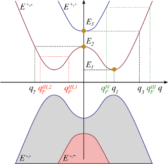
Figure 7: (color online) Schematic representation of an arbitrary cut of the bandstructure of bilayer graphene close to the Dirac point.

Appendix B Energy Integrals

To compute the total electronic energy, the evaluation of the integral

$$F^{\pm,\pm}\equiv\pm\frac{1}{2}\int kdk\sqrt{A+Bk^{2}\pm 2\sqrt{D+Ek^{2}}}$$ (32)

is required. The parameters, with respect to the dispersion of the bilayer in Eq. (6), are given as

$$A=V^{2}+2t_{\perp}^{2}\,,\quad B=4\nu_{F}^{2}\,,\quad D=t_{\perp}^{4}\,,$$

$$E=4\nu_{F}^{2}(tp^{2}+V^{2})\,.$$ (33)

The integral is readily computed by changing to the variable $x\equiv\sqrt{D+Ek^{2}}$, after which it becomes

$$\int xdx\sqrt{\alpha+\beta x+\gamma x^{2}}\,,$$ (34)

and is readily available in standard tables. The final result is thus

$$F^{\eta_{1},\eta_{2}} =\frac{\eta_{1}}{4\nu_{F}^{2}(t_{\perp}^{2}+V^{2})}\biggl{\{}\frac{R^{3/2}}{3\gamma}-\frac{\gamma x+\eta_{2}}{2\gamma^{2}}\eta_{2}\sqrt{R}$$

$$-\frac{\eta_{2}\Delta}{8\gamma^{5/2}}\log\Bigl{(}2\sqrt{\gamma R}+2\gamma x+2\eta_{2}\Bigr{)}\biggr{\}}\,,$$ (35)

where

$$R \equiv\alpha+\beta x+\gamma x^{2}\,,$$

$$\Delta \equiv 4\alpha\gamma-\beta^{2}=\frac{4V^{2}t_{\perp}^{2}}{(t_{\perp}^{2}+V^{2})^{2}}\,,$$

$$\alpha \equiv A-\frac{BD}{E}=\frac{V^{4}+t_{\perp}^{4}+3t_{\perp}^{2}V^{2}}{t_{\perp}^{2}+V^{2}}\,,$$

$$x \equiv\sqrt{t_{\perp}^{4}+4\nu_{F}^{2}(t_{\perp}^{2}+V^{2})k^{2}}\,,$$

$$\gamma =\frac{1}{t_{\perp}^{2}+V^{2}}\,,$$

$$\beta =\pm 2\,.$$ (36)

References

- Castro Neto et al. (2007) A. H. Castro Neto, F. Guinea, N. M. R. Peres, K. S. Novoselov, and A. K. Geim, arXiv:0709.1163 (2007).
- Novoselov et al. (2004) K. S. Novoselov, A. K. Geim, S. V. Morozov, D. Jiang, Y. Zhang, S. V. Dubonos, I. V. Grigorieva, and A. A. Firsov, Science 306, 666 (2004).
- Novoselov et al. (2005a) K. S. Novoselov, A. K. Geim, S. V. Morozov, D. Jiang, M. I. Katsnelson, I. V. Grigorieva, S. V. Dubonos, and A. A. Firsov, Nature 438, 197 (2005a).
- Novoselov et al. (2005b) K. S. Novoselov, D. Jiang, F. Schedin, T. J. Booth, V. V. Khotkevich, S. V. Morozov, and A. K. Geim, Proc. Natl. Acad. Sci. USA 102, 10453 (2005b).
- Castro Neto et al. (2006) A. H. Castro Neto, F. Guinea, and N. M. R. Peres, Physics World 19, 33 (2006).
- Katsnelson and Novoselov (2007) M. I. Katsnelson and K. S. Novoselov, Solid State Commun. 143, 3 (2007).
- Morozov et al. (2008) S. V. Morozov, K. S. Novoselov, M. I. Katsnelson, F. Schedin, D. C. Elias, J. A. Jaszczak, and A. K. Geim, Phys. Rev. Lett. 100, 016602 (2008).
- Novoselov et al. (2006) K. S. Novoselov, E. McCann, S. V. Morozov, V. I. Fal’ko, M. I. Katsnelson, U. Zeitler, D. Jiang, F. Schedin, and A. K. Geim, Nat. Phys. 2, 177 (2006).
- Ohta et al. (2006) T. Ohta, A. Bostwick, T. Seyller, K. Horn, and E. Rotenberg, Science 313, 5789 (2006).
- McCann (2006) E. McCann, Phys. Rev. B 74, 161403R (2006).
- Castro et al. (2007) E. V. Castro, K. S. Novoselov, S. V. Morozov, N. M. R. Peres, J. M. B. L. dos Santos, J. Nilsson, F. Guinea, A. K. Geim, and A. H. Castro Neto, Phys. Rev. Lett. 99, 216802 (2007).
- Oostinga et al. (2008) J. B. Oostinga, H. B. Heersche, X. Liu, A. F. Morpurgo, and L. M. K. Vandersypen, Nat. Mater. 7, 151 (2008).
- Su et al. (1979) W. P. Su, J. R. Schrieffer, and A. J. Heeger, Phys. Rev. Lett. 42, 1698 (1979).
- Su et al. (1980) W. P. Su, J. R. Schrieffer, and A. J. Heeger, Phys. Rev. B 22, 2099 (1980).
- Fincher et al. (1978) C. R. Fincher, D. L. Peebles, A. J. Heeger, M. A. Druy, Y. Matsumura, A. G. MacDiarmid, H. Shirakawa, and S. Ikeda, Solid State Commun. 27, 489 (1978).
- Rutter et al. (2007) G. M. Rutter, J. N. Crain, N. P. Guisinger, T. Li, P. N. First, and J. A. Stroscio, Science 317, 219 (2007).
- Dresselhaus and Dresselhaus (2002) M. S. Dresselhaus and G. Dresselhaus, Adv. Phys. 51, 1 (2002).
- Wirtz and Rubio (2004) L. Wirtz and A. Rubio, Solid State Commun. 131, 141 (2004).
- Jansen and Freeman (1987) H. J. F. Jansen and A. J. Freeman, Phys. Rev. B 35, 8207 (1987).
- Boettger (1997) J. C. Boettger, Phys. Rev. B 55, 11202 (1997).
- Mounet and Marzari (2005) N. Mounet and N. Marzari, Phys. Rev. B 71, 205214 (2005).
- Nemanich et al. (1977) R. J. Nemanich, G. Lucovsky, and S. A. Solin, Mat. Sci. and Eng. 31, 157 (1977).
- Fuchs and Lederer (2007) J.-N. Fuchs and P. Lederer, Phys. Rev. Lett. 98, 016803 (2007).
- Slater and Koster (1954) J. C. Slater and G. F. Koster, Phys. Rev. 94, 1498 (1954).
- Harrison (1999) W. A. Harrison, Elementary Electronic Structure (World Scientific, 1999).
- Kim and Castro Neto (2007) E.-A. Kim and A. H. Castro Neto, arXiv:cond-mat/0702562 (2007).
- Papaconstantopoulos et al. (1998) D. A. Papaconstantopoulos, M. J. Mehl, S. C. Erwin, and M. R. Pederson, in Tight-Binding Approach to Computational Materials Science, edited by P. Turchi, A. Gonis, and L. Colombo (Materials Research Society, Pittsburgh, 1998), p. 221.
- Ohta et al. (2007) T. Ohta, A. Bostwick, J. L. McChesney, T. Seyller, K. Horn, and E. Rotenberg, Phys. Rev. Lett. 98, 206802 (2007).
- Malard et al. (2007) L. M. Malard, J. Nilsson, D. C. Elias, J. C. Brant, F. Plentz, E. S. Alves, A. H. C. Neto, and M. A. Pimenta, Phys. Rev. B 76, 201401 (2007).
- Yan et al. (2007) J. Yan, E. A. Henriksen, P. Kim, and A. Pinczuk, arXiv:0712.3879 (2007).
- Lazzeri et al. (2008) M. Lazzeri, C. Attaccalite, L. Wirtz, and F. Mauri, Phys. Rev. B 78, 081406 (2008).
- Monkhorst and Pack (1968) H. J. Monkhorst and J. D. Pack, Phys. Rev. B 13, 5188 (1968).
- Hartwigsen et al. (1998) C. Hartwigsen, S. Goedecker, and J. Hutter, Phys. Rev. B 58, 3641 (1998).