Large N transition in the 2D SU(N)xSU(N) nonlinear sigma model.

Abstract:

We consider the characteristic polynomial associated with the smoothed two point function in two dimensional large $N$ principal chiral model. We numerically show that it undergoes a transition at a critical distance of the order of the correlation length. The transition is in the same universality class as two dimensional large $N$ QCD.

1 Two dimensional SU(N) X SU(N) principal chiral model

The two dimensional SU(N) X SU(N) principal chiral model is similar to four dimensional SU(N) gauge theory in many respects[1]. The continuum action is given by

$$S=\frac{N}{T}\int d^{2}xTr\partial_{\mu}g(x)\partial_{\mu}g^{\dagger}(x)$$ (1)

where $g(x)\in$ SU(N). The global symmetry group SU(N)${}_{L}\times$ SU(N)_R reduces down to a single SU(N) “diagonal subgroup” if we make a translation breaking “gauge choice”, $g(0)=1$. This model is asymptotically free and there are $N-1$ particle states with masses

$$M_{R}=M\frac{\sin(\frac{R\pi}{N})}{\sin(\frac{\pi}{N})},~{}~{}~{}1\leq R\leq N-1.$$ (2)

The states corresponding to the $R$-th mass are a multiplet transforming as an $R$ component antisymmetric tensor of the diagonal symmetry group.

The two point function $W=g(0)g^{\dagger}(x)$ plays the role of Wilson loop with the separation $x$ playing the role of area. We expect the behavior to be perturbative for small $x$. On the other hand, non-perturbative effects become important for large $x$.

One expects

$$G_{R}(x)=\langle\chi_{R}(g(0)g^{\dagger}(x))\rangle\sim C_{R}{N\choose R}e^{-M_{R}|x|}$$ (3)

where $\chi_{R}$ is the trace in the $R$-antisymmetric representation. Comparison with the heat-kernel representation of the characteristic polynomial associated with the Wilson loop operator in two dimensional large $N$ QCD [2] suggests the following connections:

• The two point correlator, $W(d)=g(0)g^{\dagger}(d)$, is analogous to the Wilson loop operator.

• $M|x|$ is analogous to the dimensionless area, $t$.

Based on this analogy, we hypothesize [3] that the characteristic polynomial, $\det\left(z-g(0)g^{\dagger}(d)\right)$, will undergo a transition at some value $d_{c}$. The universal behavior at this transition will be in the same universality class as two dimensional large $N$ QCD.

2 Setting the scale

Numerical measurement of the correlation length using the lattice action

$$S_{L}=-2Nb\sum_{x,\mu}\Re Tr[g(x)g^{\dagger}(x+\mu)]$$ (4)

and

$$\xi_{G}^{2}=\frac{1}{4}\frac{\sum_{x}x^{2}G_{1}(x)}{\sum_{x}G_{1}(x)}$$ (5)

yields the following continuum result [4]:

$$M\xi_{G}=0.991(1)$$ (6)

We use $\xi_{G}$ to set the scale and it is well described by

$$\xi_{G}=0.991~{}\left[\frac{e^{\frac{2-\pi}{4}}}{16\pi}\right]~{}\sqrt{E}~{}\exp\left(\frac{\pi}{E}\right)$$ (7)

in the range $11\leq\xi_{G}\leq 20$ with

$$E=1-\frac{1}{N}\Re\langle Tr[g(0)g^{\dagger}({\hat{1}})]\rangle=\frac{1}{8b}+\frac{1}{256b^{2}}+\frac{0.000545}{b^{3}}-\frac{0.00095}{b^{4}}+\frac{0.00043}{b^{5}}$$ (8)

The above equations will be used to find a $b$ for a given $\xi$.

3 Smeared SU(N) matrices

Well defined operators are obtained using smeared matrices. We start with $g(x)\equiv g_{0}(x)$ and one smearing step takes us from $g_{t}(x)$ to $g_{t+1}(x)$ using the following procedure. Define $Z_{t+1}(x)$ by:

$$Z_{t+1}(x)=\sum_{\pm\mu}[g^{\dagger}_{t}(x)g_{t}(x+\mu)-1].$$ (9)

Construct anti-hermitian traceless $SU(N)$ matrices $A_{t+1}(x)$

$$A_{t+1}(x)=Z_{t+1}(x)-Z^{\dagger}_{t+1}(x)-\frac{1}{N}\rm{Tr}(Z_{t+1}(x)-Z^{\dagger}_{t+1}(x))\equiv-A^{\dagger}_{t+1}(x).$$ (10)

Set

$$L_{t+1}(x)=\exp[{fA_{t+1}(x)}].$$ (11)

$g_{t+1}(x)$ is defined in terms of $L_{t+1}(x)$ by:

$$g_{t+1}(x)=g_{t}(x)L_{t+1}(x).$$ (12)

This procedure is iterated till we reach $g_{n}(x)$ and the smearing parameter is defined by $\tau=nf$. For a fixed $\xi_{G}$, the parameter $\tau$ is fixed such that $\tau/\xi_{G}^{2}$ remains unchanged. We set $n=30$ in our numerical simulations and this was found sufficiently large to eliminate a dependence on the two factors, $f$ and $n$, individually.

4 Numerical details

We need $L/\xi_{G}>7$ to minimize finite volume effects. We worked in the range $11\leq\xi_{G}\leq 20$ and therefore we chose $L=150$. We used a combination of Metropolis and over-relaxation at each site $x$ for our updates. The full SU(N) group was explored. 200-250 passes of the whole lattices were sufficient to thermalize starting from $g(x)\equiv 1$. 50 passes per step were enough to equilibrate if $\xi_{G}$ was increased in steps of $1$.

The test of the universality hypothesis proceeds in the same manner as for the three dimensional large $N$ gauge theory. We defined the characteristic polynomial, $F(y,d)$, as

$$F(y,d)=\langle\det(e^{y/2}+e^{-y/2}W(d))\rangle$$ (13)

We perform a Taylor expansion,

$$F(y,d,N)=C_{0}(d,N)+C_{2}(d,N)y^{2}+C_{4}(d,N)y^{4}+\dots$$ (14)

since $F(y,d)$ is an even function of $y$. It is useful to define

$$\Omega(d,N)=\frac{C_{0}(d,N)C_{4}(d,N)}{C_{2}^{2}(d,N)}$$ (15)

which resembles a Binder cumulant.

As $N\to\infty$, $\Omega(d,\infty)$ is a step function with $\Omega=\frac{1}{6}$ for short distances $d<d_{c}$ and $\Omega=\frac{1}{2}$ for long distances, $d>d_{c}$. Zooming in on the step function as $N\to\infty$ in the vicinity of $d=d_{c}$ using the scaling variable $\alpha\propto\sqrt{N}(d-d_{c})$, we obtain Fig. 1.

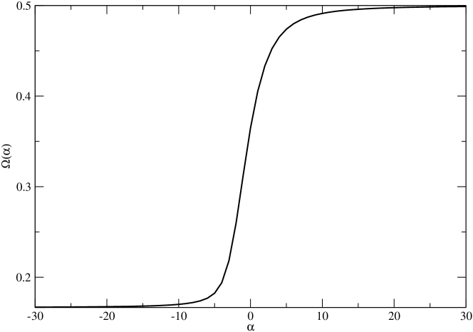
Figure 1: Behavior of $\Omega$ as a function of $\alpha$ in the scaling region.

We use $\Omega(\alpha=0)=0.364739936$ to obtain the critical size $d_{c}$ in the following manner. Given an $N$ and a $\xi$, we find the $d_{c}$ that makes the Binder cumulant $\Omega(d_{c},N)=0.364739936$ as shown in Fig. 2.

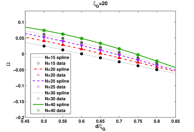
Figure 2: Plot of $\Omega(d)$ after the subtraction of $\Omega(\alpha=0)=0.364739936$ as a function of $d/\xi_{G}$.

We look at $d_{c}$ as a function of $\xi$ for a given $N$. This gives us the continuum value of $d_{c}/\xi$ for that $N$. This extrapolation is shown in Fig. 3 for $N=30$.

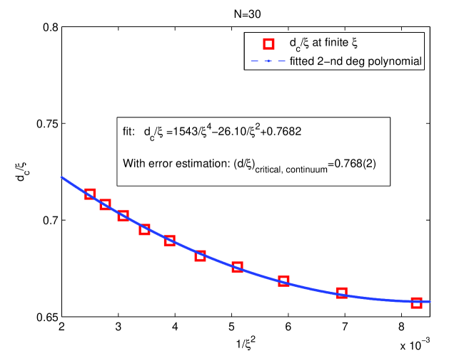
Figure 3: Extrapolation to continuum of $d_{c}/\xi$ for $N=30$.

We then take the large $N$ limit as shown in Fig. 4 and it gives us

$$\frac{d_{c}}{\xi_{G}}|_{N=\infty}=0.885(3)$$ (16)

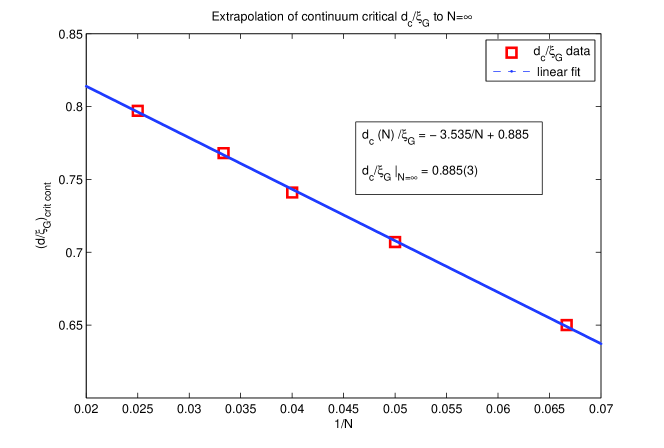
Figure 4: Extrapolation of the continuum $d_{c}/\xi$ to infinite $N$.

Further substantiation of the universal behavior can be given by comparing the eigenvalues distribution in the model to the Durhuus-Olesen eigenvalue distributions in two dimensional QCD. This is shown for one example each on either side of the critical point in Fig. 5 and very close to the critical point in Fig. 6. We use $2k=t$ to match with the notation in [5].

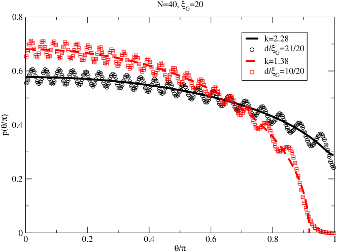
Figure 5: Examples of eigenvalue distribution for one small and one large distance.

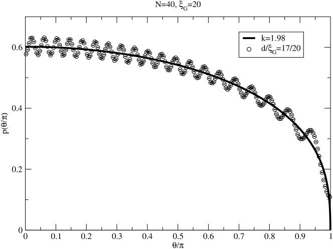
Figure 6: An example of an almost critical eigenvalue distribution.

- [1] P. Rossi, M. Campostrini and E. Vicari, Phys. Rept. 302, 143 (1998) [arXiv:hep-lat/9609003].
- [2] R. Narayanan and H. Neuberger, JHEP 0712, 066 (2007) [arXiv:0711.4551 [hep-th]].
- [3] R. Narayanan, H. Neuberger and E. Vicari, JHEP 0804, 094 (2008) [arXiv:0803.3833 [hep-th]].
- [4] P. Rossi and E. Vicari, Phys. Rev. D 49, 1621 (1994) [Erratum-ibid. D 55, 1698 (1997)] [arXiv:hep-lat/9307014].
- [5] B. Durhuus and P. Olesen, Nucl. Phys. B 184, 461 (1981).