Universal properties of Wilson loop operators in large N QCD

Abstract:

Eigenvalues of a Wilson loop operator are gauge invariant and their distribution undergoes a transition at infinite $N$ as the size of the loop is changed. We study this transition using the average characteristic polynomial associated with the Wilson loop operator. We derive the scaling function in a certain double scaling limit for two dimensional QCD and hypothesize that the transition in three and four dimensional QCD are in the same universality class. Numerical evidence for this hypothesis is provided in three dimensions.

1 Introduction

In this talk, we present the main idea in [1] and provide a sampling of the numerical results.

The Wilson loop operator, $W$, is a unitary operator for SU(N) gauge theories and can be used as a probe of the transition from strong coupling to weak coupling. Large (area) Wilson loops are non-perturbative and correspond to strong coupling. Small (area) Wilson loops are perturbative and correspond to weak coupling.

The probe is defined as

$${\cal W}_{N}(z,b,L)=\langle\det(z-W)\rangle$$ (1)

and is the characteristic polynomial associated with the operator. $W$ is the Wilson loop operator, $z$ is a complex number, $N$ is the number of colors, $b=\frac{1}{g^{2}N}$ is the lattice gauge coupling and $L$ is the linear size of the square loop. $\langle\cdots\rangle$ is the average over all gauge fields with the standard gauge action.

The eigenvalues of $W$ are gauge invariant and so is the characteristic polynomial. The eigenvalues lie on the unit circle and all of them will be close to unity for small loops. The eigenvalues will spread uniformly over the unit circle for large loops. The characteristic polynomial exhibits a transition at $N=\infty$ when $L\to L_{c}(b)$. This is a physical transition since $L_{c}(b)$ will scale properly with the coupling, $b$, as one approaches the continuum limit.

The scaling function in the double scaling limit can be derived for two dimensional large $N$ QCD [1]. We have numerically shown that three dimensional QCD falls into the same universality class [1].

2 Two dimensional QCD and a multiplicative matrix model

Two dimensional gauge theory on an infinite lattice can be gauge fixed so that the only variables are the individual plaquettes and these will be independently and identically distributed. $W=\prod_{j=1}^{n}U_{j}$ where $U_{j}$s are the transporters around the individual plaquettes that make up the loop and $n=L^{2}$ is equal to the area of the loop. The measure associated with $U_{j}$ can be set to $P(U_{j})={\cal N}e^{-\frac{N}{2}{\rm Tr\ }H_{j}^{2}}$ where $U_{j}=e^{i\epsilon H_{j}}$ and $\epsilon$ plays the role of gauge coupling. The dimensionless area is given by $t=\epsilon^{2}n$ which is kept fixed as one takes the limit $n\to\infty$ and $\epsilon\to 0$. This is called the multiplicative matrix model [2]. In the continuum limit, the parameters $b$ and $L$ get replaced by one parameter, which is denoted by $t$ in the model, and the characteristic polynomial becomes

$${\cal W}_{N}(z,b,L)\to Q_{N}(z,t)$$

3 Average characteristic polynomial

Using a fermionic representation of the determinant, one can perform the integration over $U_{j}$. One can then perform the integration over the fermionic variables to obtain the following result for the characteristic polynomial:

$$Q_{N}(z,t)=\cases{\sqrt{\frac{N\tau}{2\pi}}\int_{-\infty}^{\infty}d\nu e^{-\frac{N}{2}\tau\nu^{2}}\left[z-e^{-\tau\nu-\frac{\tau}{2}}\right]^{N}&$SU(N)$\cr\sqrt{\frac{Nt}{2\pi}}\int_{-\infty}^{\infty}d\nu e^{-\frac{N}{2}t\nu^{2}}\left[z-e^{-t\nu-\frac{\tau}{2}}\right]^{N}&$U(N)$\cr}$$ (2)

Integrating out $\nu$ gives exact continuum polynomial expressions,

$$Q_{N}(z,t)=\cases{\sum_{k=0}^{N}\pmatrix{N\cr k\cr}z^{N-k}(-1)^{k}e^{-\frac{\tau k(N-k)}{2N}}&$SU(N)$\cr\sum_{k=0}^{N}\pmatrix{N\cr k\cr}z^{N-k}(-1)^{k}e^{-\frac{tk(N+1-k)}{2N}}&$U(N)$\cr}$$ (3)

$$\tau=t\left(1+\frac{1}{N}\right)$$ (4)

4 Heat-kernel measure

The result for $Q_{N}(z,t)$ is consistent with the heat-kernel measure for $W$:

$$P(W,\tau)dW=\sum_{R}d_{R}\chi_{R}(W)e^{-\tau C_{2}(R)}dW.$$ (5)

$R$ denotes the representation, $d_{R}$ is the dimension of the representation $R$ and $C_{2}(R)$ is the second order Casimir in the representation $R$. To see this, note that

$$Q_{N}(z,t)=\langle\prod_{j=1}^{N}(z-e^{i\theta_{j}})\rangle=\sum_{k=0}^{N}z^{N-k}(-1)^{k}M_{k}(t).$$ (6)

If we now take the average, $\langle\cdots\rangle$ over the heat-kernel measure, we get

$$M_{k}(t)=\langle\sum_{1\leq j_{1}<j_{2}<j_{3}....<j_{k}\leq N}e^{i(\theta_{j_{1}}+\theta_{j_{2}}+...+\theta_{j_{k}})}\rangle=\langle\chi_{k}(W)\rangle=d_{k}e^{-\tau C_{2}(k)}={N\choose k}e^{-\frac{\tau k(N-k)}{2N}}$$ (7)

5 Zeros of $Q_{N}(z,t)$

Since $W$ is a unitary operator, the zeros of $\det(z-W)$ will lie in the unit circle. One can show this remains true for $Q_{N}(z,t)$ when the gauge group is $SU(N)$. To see this, we rewrite $Q_{N}(z,t)$ for $SU(N)$ as

$$Z_{N}(z,t)=Q_{N}(z,t)(-1)^{N}e^{\frac{(N-1)\tau}{8}}(-z)^{-\frac{N}{2}}=\sum_{\sigma_{1},\sigma_{2},...\sigma_{N}=\pm\frac{1}{2}}e^{\ln(-z)\sum_{i}\sigma_{i}}e^{\frac{\tau}{N}\sum_{i>j}\sigma_{i}\sigma_{j}}$$ (8)

This is the partition function for a spin model with a ferromagnetic interaction for positive $\tau$. $ln(-z)$ is a complex external magnetic field. Therefore, the conditions for Lee-Yang theorem [3] are fulfilled and all roots of $Q_{N}(z,t)$ lie on the unit circle for SU(N). This is not the case for U(N).

6 Weak coupling vs strong coupling

The transition from weak coupling to strong coupling can be intuitively seen using the characteristic polynomial, $Q_{N}(z,t)$. In the weak coupling (small area) limit we have $t=0$ and $Q_{N}(z,t)=(z-1)^{N}$. Therefore, all roots are at $z=1$ on the unit circle. In the strong coupling (large area) limit we have $t=\infty$ and $Q_{N}(z,t)=z^{N}+(-1)^{N}$. Therefore, all roots are uniformly distributed on the unit circle.

$Q_{N}(z,t)$ is analytic in $z$ for all $t$ at finite $N$. But, this is not the case as $N\to\infty$ and this leads to a transition from weak to strong coupling in the $N\to\infty$ limit.

7 Phase transition in an observable – Durhuus-Olesen transition

There is a critical area, $t=4$, such that the distribution of zeros of $Q_{\infty}(z,t)$ on the unit circle has a gap around $z=-1$ for $t<4$ and has no gap for $t>4$ [2, 4]. To see this, we note that the integral representation (2) is dominated by the saddle point, $\nu=\lambda(t,z)$, given by

$$\lambda=\lambda(t,z)=\frac{1}{ze^{t(\lambda+\frac{1}{2})}-1}$$ (9)

With $z=e^{i\theta}$ and $w=2\lambda+1$, $\rho(\theta)=-\frac{1}{4\pi}{\bf Re}\ w$ gives the distribution of the eigenvalues of $W$ on the unit circle.

The saddle point equation at $z=-1$ is

$$w=\tanh\frac{t}{4}w$$ (10)

showing that $w$ admits non-zero real solutions for $t>4$.

8 Double scaling limit

As $N\to\infty$, one can define a scaling region around $t=4$ and $z=-1$ by

$$t=\frac{4}{1+\frac{\alpha}{\sqrt{3N}}};\ \ \ \ z=-e^{\left(\frac{4}{3N}\right)^{\frac{3}{4}}\xi}$$ (11)

$\alpha$ and $\xi$ are the scaling variables that blow up the region near $t=4$ and $z=-1$. We can show that

$$\lim_{N\rightarrow\infty}\left(\frac{4N}{3}\right)^{\frac{1}{4}}(-1)^{N}e^{\frac{(N-1)\tau}{8}}(-z)^{-\frac{N}{2}}Q_{N}(z,t)=\int_{-\infty}^{\infty}due^{-u^{4}-\alpha u^{2}+\xi u}\equiv\zeta(\xi,\alpha)$$ (12)

which is the scaling function in the double scaling limit associated with the characteristic polynomial.

We hypothesize that this behavior in the double scaling limit derived for two dimensional large $N$ QCD is universal and should be seen in the large $N$ limit of 3D QCD, 4D QCD, 2D PCM and other related models. The modified Airy function, $\zeta(\xi,\alpha)$, is the universal scaling function.

9 Large N universality hypothesis

We can now precisely state the continuum large $N$ universality hypothesis that can be numerically tested in relevant models.

Let ${\cal C}$ be a closed non-intersecting loop: $x_{\mu}(s),s\in[0,1]$. Let ${\cal C}(m)$ be a whole family of loops obtained by dilation: $x_{\mu}(s,m)=\frac{1}{m}x_{\mu}(s)$,with $m>0.$ Let $W(m,{\cal C}(*))=W({\cal C}(m))$ be the family of operators associated with the family of loops denoted by ${\cal C}(*)$ where $m$ labels one member in the family. Define

$$O_{N}(y,m,{\cal C}(*))=\langle\det(e^{\frac{y}{2}}+e^{-\frac{y}{2}}W(m,{\cal C}(*))\rangle$$ (13)

Then our hypothesis is

$$\lim_{N\rightarrow\infty}{\cal N}(N,b,{\cal C}(*))O_{N}\left(y=\left(\frac{4}{3N^{3}}\right)^{\frac{1}{4}}\frac{\xi}{a_{1}({\cal C}(*))},m=m_{c}\left[1+\frac{\alpha}{\sqrt{3N}a_{2}({\cal C}(*))}\right]\right)=\zeta(\xi,\alpha)$$ (14)

10 Numerical test of the universality hypothesis – 3D large N QCD

We use standard Wilson gauge action. The lattice coupling $b=\frac{1}{g^{2}N}$ has dimensions of length. We use square Wilson loops of linear length $L$. We change $b$ to generate a family of square loops labeled by $L$. While doing this, we need to keep $0.42<b<b(V)$ where $V$ is the lattice volume assumed large enough for large $N$ continuum reduction to hold in the confined phase [5, 6]. We use smeared links in the construction of the Wilson loop operator to avoid corner and perimeter divergences.

We obtain $b_{c}(L)$, $a_{1}(L)$ and $a_{2}(L)$ such that

$$\lim_{N\rightarrow\infty}{\cal N}(b,N)O_{N}\left(y=\left(\frac{4}{3N^{3}}\right)^{\frac{1}{4}}\frac{\xi}{a_{1}(L)},b=b_{c}(L)\left[1+\frac{\alpha}{\sqrt{3N}a_{2}(L)}\right]\right)=\zeta(\xi,\alpha)$$ (15)

This is done by fixing $N$ and $L$ and obtaining estimates for $b_{c}(L,N)$, $a_{1}(L,N)$ and $a_{2}(L,N)$. We then take the limit as $N\to\infty$ and we check that $b_{c}(L)$, $a_{1}(L)$ and $a_{2}(L)$ have proper continuum limits as $L\to\infty$. The extrapolation to the continuum limit are shown in Fig. 1, Fig. 2 and Fig. 3.

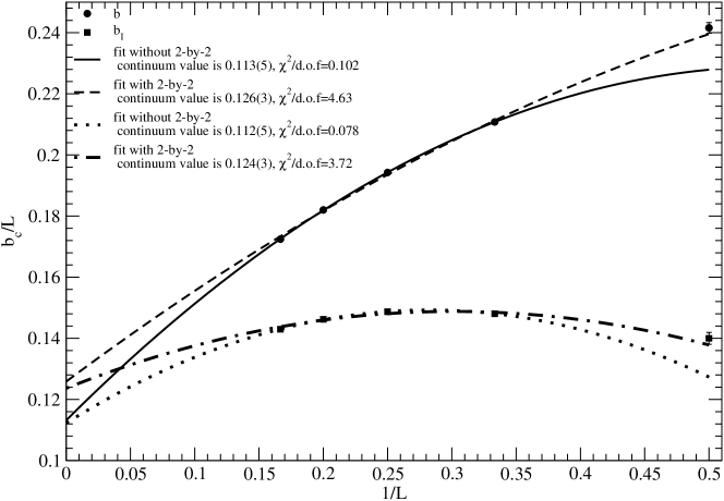
Figure 1: Extrapolation to the continuum limit of the critical area.

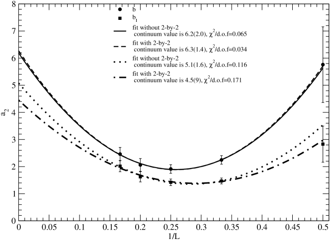
Figure 2: Extrapolation to the continuum limit of the parameter matching to the scaled variable, $\alpha$.

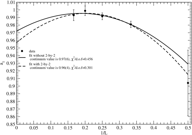
Figure 3: Extrapolation to the continuum limit of the parameter matching to the scaled variable, $\xi$.

- [1] R. Narayanan and H. Neuberger, JHEP 0712, 066 (2007) [arXiv:0711.4551 [hep-th]].
- [2] R. A. Janik, W. Wieczorek, J. Phys. A: Math. Gen. 37, 6521 (2004).
- [3] T. D. Lee and C. N. Yang, Phys. Rev. 87, 410 (1952).
- [4] B. Durhuus and P. Olesen, Nucl. Phys. B 184, 461 (1981).
- [5] R. Narayanan and H. Neuberger, Phys. Rev. Lett. 91, 081601 (2003) [arXiv:hep-lat/0303023].
- [6] R. Narayanan, H. Neuberger and F. Reynoso, Phys. Lett. B 651, 246 (2007) [arXiv:0704.2591 [hep-lat]].