Explicit R-Symmetry Breaking and Metastable Vacua

Abstract

We consider O’Raifeartaigh-like models with explicit R-symmetry breaking and analyze the vacuum landscape. Taking such models as candidates for the hidden sector, we analyze the gauge mediation of the supersymmetry breaking, focusing on the effects produced by R-symmetry breaking. First, we construct families of non-R-symmetric models containing only singlet chiral superfields, and determine the conditions under which SUSY vacua, runaway directions and (longlived) metastable vacua exist. We then extend the results to the case in which some of the chiral fields are in the $5\oplus\bar{5}$ representation of $SU(5)$. Gauging this symmetry, we compute soft masses for gauginos and sfermions, and analyze several issues such as doublet/triplet splitting, unification of coupling constants and CP violation phases.

1 Introduction

The fact that supersymmetry (SUSY) breaking is intimately tied to the existence of a global $U(1)$ R-symmetry was first stressed in the work of Nelson and Seiberg [1], where it was shown that in order to have SUSY breaking in generic models there must be an R-symmetry, and the spontaneous breaking of this latter symmetry is a sufficient condition for the existence of non supersymmetric vacua. As it is well known, if supersymmetry is realized in nature, it must be broken. Concerning R-symmetry, generation of gaugino masses requires that it should be broken, either explicitly or spontaneously.

It was recently shown in ref. [2] that metastable supersymmetry breaking is generic in supersymmetric field theory and highly simplifies model-building. Moreover, there is a growing consensus on the fact that such metastable supersymmetry breaking takes place in a hidden sector of the full theory, and its effects are communicated to the visible sector (MSSM) through gauge interactions with messenger fields (this is the gauge mediation scenario [3]-[12], see for example [13] for a review).

It should be stressed that metastability is closely related to R-symmetry breaking. Concerning explicit R-symmetry breaking, stable SUSY breaking vacua can become metastable in generic models since in that case SUSY vacua can appear [1]. Metastable vacua also exist when R-symmetry is spontaneously broken, for example by assigning generic R-charges to fields [14] or by coupling the model to some broken gauge symmetry [15], [16]. There is yet another possibility in the field of R-breaking which is that pseudo-moduli are only sensitive to two-loops in perturbation theory [17].

As discussed in [18], the way in which R-symmetry is broken (explicitly or spontaneously) leaves a clear imprint on the phenomenology of the minimal supersymmetric standard model (MSSM) and it is then of interest to study broad classes of such models so as to compare the resulting patterns.

In the present paper we shall follow the gauge mediation route, choosing for the hidden sector (non-generic) O’Raifeartaigh-type models [19]. R-symmetry will be broken explicitly and in this sense our study can be seen as complementary to that of ref. [20], where the R-breaking mechanism is spontaneous. We start by constructing families of non-R-symmetric models containing only singlet chiral superfields to describe the hidden sector. A detailed analysis of the vacuum landscape will allow us to determine the conditions under which SUSY vacua, runaway directions and longlived metastable vacua exist.

In order to promote these models to more realistic candidates for the SUSY breaking sector, we also consider the case in which some of the chiral fields are in the $5\oplus\bar{5}$ representation of $SU(5)$, leaving the field which triggers SUSY breaking as a singlet spurion. By gauging the $SU(5)$ flavor symmetry, we allow some fields to interact through gauge loops with the MSSM fields. We compute soft masses and analyze issues such as doublet/triplet splitting, unification of coupling constants and CP violation phases.

The paper is organized as follows. In section 2 we discuss three families of non-R-symmetric O’Raifeartaigh-like models, having different messenger mass matrices and all chiral superfields (messengers and spurion) taken as singlets. Then, in section 3 we extend the analysis by considering the case in which messengers are taken in the $\bar{5}\oplus 5$ representation of $SU(5)$. Section 4 addresses to the analysis of gauge mediation. Finally, in section 5 we summarize and discuss our results.

2 O’Raifeartaigh-like models with explicit R-symmetry breaking

The O’Raifeartaigh model [19], a paradigm of SUSY breaking, is a theory with three chiral superfields $X$, $\phi_{1}$, $\phi_{2}$ transforming under a global $U(1)_{R}$

$$\Phi(\theta)\to e^{iR(\Phi)\alpha}\Phi(e^{-i\alpha}\theta)\ ,$$ (1)

with charges $R(X)=2,\ R(\phi_{1})=0,\ R(\phi_{2})=2$, a canonical Kähler potential and a superpotential of the form

$$W_{O^{\prime}R}=\frac{\lambda}{2}X\phi_{1}^{2}+m\phi_{1}\phi_{2}+fX\ .$$ (2)

Here $\lambda,m,f$ are complex. The model is renormalizable, R-symmetric and not generic (not all the terms consistent with R-symmetry are present, for example $X\phi_{1},\ \phi_{2}\phi_{1}^{2},\ \phi_{2}$ are absent). The field $X$, usually called a spurion, acquires a non-vanishing F-component, triggering SUSY breaking

$$X=X+\theta^{2}F\ .$$ (3)

When $\lambda f<m^{2}$ there is a phase in which supersymmetry is spontaneously broken at

$$\phi_{1}=\phi_{2}=0\,,\ \ \ \ F=f\,,\ \ \ \ \forall\ X\ ,$$ (4)

and there are neither supersymmetric vacua nor runaway directions. At the tree level there is a one-dimensional moduli space of degenerate non-supersymmetric vacua parameterized by $X$. This result is general, non-SUSY tree-level vacua is always degenerate in Wess-Zumino models [21]-[22]. The degeneracy is then lifted à la Coleman-Weinberg [23] when quantum corrections are taken into account. At one loop, the vacuum expectation value (VEV) of the $X$ field vanishes (as it happens for $\phi_{1}$ and $\phi_{2}$) and then the R-symmetry is not spontaneously broken. In addition there is another phase when $\lambda f>m^{2}$ containing two disjoint pseudo-moduli spaces, also lifted in such a way that the R-symmetry remains unbroken. We shall not analyze this last phase of the O’Raifeartaigh model.

In order to test different possibilities of SUSY breaking, this model has been generalized in many ways, by adding fields and/or considering generic superpotentials. For example, in [15] the following superpotential with $r$ fields $X_{i}$ and $s$ fields $\phi_{j}$ with R-charges $2$ and $0$ respectively has been proposed

$$W=\sum_{i=1}^{r}X_{i}\ g_{i}(\phi_{j})\ ,\ \ \ \ \ j=1,\dots,s\ .$$ (5)

Here the functions $g_{i}$ are generic and supersymmetry is broken with an $(r-s)$-dimensional moduli space of non-supersymmetric vacua parameterized by $X_{i}$. As in the previous case, this degeneracy is lifted at the quantum level in such a way that R-symmetry remains unbroken. As shown in [15], coupling the $X$ field to a broken gauge symmetry leads to a vacuum with $X_{i}\neq 0$, thus breaking R symmetry spontaneously. The possibility of explicit (and small) R-symmetry breaking was considered in that paper [15] and in [24].

In [14], a particular generalization to the O’Raifeartaigh superpotential (2) was presented

$$W=fX+\frac{1}{2}(M_{ij}+XN_{ij})\phi_{i}\phi_{j}\ ,\;\;\;\;i,j=1,2,\ldots,N_{\phi}\ .$$ (6)

Here $f\neq 0$ is a complex parameter, $M$ and $N$ symmetric complex matrices and $\det M\neq 0$. For future reference, we define $N_{R}$ as the number of distinct R-charges carried by the $\phi$-fields. R-symmetry is guaranteed by requiring $R(X)=2$ and constraining $M$ and $N$ in such a way that

$${\rm if~{}}M_{ij}\neq 0\ {\rm~{}one~{}has~{}}R(\phi_{i})+R(\phi_{j})=2\ ,$$

$${\rm if~{}}N_{ij}\neq 0\ {\rm~{}one~{}has~{}}R(\phi_{i})+R(\phi_{j})=0\ .$$ (7)

These selection rules imply that the following identity holds (see Appendix)

$$\det(M+XN)=\det(M)\ .$$ (8)

The SUSY vacua conditions are

$$f+\frac{1}{2}\ N_{ij}\ \phi_{i}\phi_{j} = 0\ ,$$ (9)

$$(M+XN)_{ij}\ \phi_{j} = 0\ .$$ (10)

As $\det M\neq 0$, equation (8) implies that (10) is only satisfied when $\phi_{j}=0$ and then SUSY is broken because it is not possible to satisfy (9) when the parameters are not fine-tuned. R-symmetry is responsible of the selection rules (7), which imply the identity (8), in which the r.h.s. is non-vanishing by definition. Then, R-symmetry is a sufficient condition for SUSY breaking, but it is not necessary since one considers a non-generic model. There is always a SUSY-breaking vacua at $\phi_{i}=0$, with a moduli space parameterized by $X$. When only R-charge $0$ and $2$ fields are present, one can show that there is a minimum of the Coleman-Weinberg effective potential at $X=0$, and then R-symmetry remains unbroken at the quantum level (it was shown in [25] that the comparison between the number of R-charge 0 and R-charge 2 is essential to the symmetry breaking properties of the model). Unbroken R-symmetry is no longer true when the possibility for generic R-charge assignments (satisfying conditions (7)) is allowed. Models with superpotential (6) were generalized to the case of many pseudo-moduli fields in [26], where it was also shown that they generically have runaway directions. The case of non-canonical Kähler potentials was analyzed in [27].

We will consider here a different extension of these models allowing the possibility of explicit R-symmetry breaking. As it is well-known [1], in generic models when R-symmetry is explicitly broken SUSY vacua always exist and those breaking SUSY could be in principle close to them. Then, since we are interested in longlived supersymmetry breaking vacua, we shall consider non-generic models with a controllable life-time. The model is defined by a canonical Kähler potential and the (non-generic) superpotential

$$W=fX+\frac{1}{2}(M+B+X(L+A))_{ij}\phi_{i}\phi_{j}\,,\;\;\;\;\;\;\;\;\;\;\;\;i,j=1,2,\ldots,N_{\phi}\ .$$ (11)

Here $f\neq 0$ is a complex parameter and $M$, $B$, $L$ and $A$ are symmetric complex matrices satisfying

$$M_{ij}\neq 0 \Rightarrow R(\phi_{i})+R(\phi_{j})=2\ ,$$

$$L_{ij}\neq 0 \Rightarrow R(\phi_{i})+R(\phi_{j})=2\ ,$$

$$B_{ij}\neq 0 \Rightarrow R(\phi_{i})+R(\phi_{j})<2\ ,$$

$$A_{ij}\neq 0 \Rightarrow R(\phi_{i})+R(\phi_{j})<2\ .$$ (12)

As before, we define $N_{R}$ as the number of distinct R-charges carried by the $\phi$-fields. Here we consider the same charge assignment as in (6) and then, as $B$, $L$ and $A$ in superpotential (11) satisfy selection rules (12) and not those required by R-symmetry (7), the models defined by (11)-(12) in general explicitly break R-symmetry. Only when $B=L=0$, $A_{ij}\neq 0$ requires $R(\phi_{i})+R(\phi_{j})=0$, and $\det M\neq 0$, the superpotential $W$ coincides with (6) and then the model is R-symmetric. In general a reassignment of R-charges might be necessary in order to check whether other choice of matrices renders the model R-symmetric (An example of this is discussed in the Appendix).

The scalar potential resulting from (11) is

$$V=|f+\frac{1}{2}(L+A)_{ij}\ \phi_{i}\phi_{j}|^{2}+|(M+B+X(L+A))_{ij}\ \phi_{j}|^{2}\ ,$$ (13)

and then the F-term conditions for SUSY vacua read

$$f+\frac{1}{2}(L+A)_{ij}\ \phi_{i}\phi_{j} = 0\ ,$$ (14)

$$(M+B+X(L+A))_{ij}\ \phi_{j} = 0\ .$$ (15)

There is a local (classical) extrema at $\phi_{i}=0\ ,\ \forall\,X$, in which $V=|f|^{2}$. At one loop, a Coleman-Weinberg potential [23] is generated on the pseudomoduli and the minima of the resulting effective potential, if they exist, will be the SUSY-breaking vacua of the theory. Notice also that if the effective potential lifts the moduli in such a way that the true minima is at $X=0$, then the R symmetry would be restored. Hence the present models provide an appropriate context to analyze R-symmetry restoration.

In principle, those SUSY breaking minima can be made longlived in the presence of SUSY vacua or runaway directions. In fact, when $X$ is such that $\det(M+B+X(L+A))\neq 0$ there is no SUSY vacua because (15) implies that $\phi=0$, which makes (14) unsolvable. In contrast, when $X$ is such that $\det(M+B+X(L+A))=0$, there is a non-zero $\phi$ solution to eq.(15) (and hence a SUSY vacuum) which can be taken far away for small entries of $L$ and $A$ in (14). The mass matrices at the extrema read

$${\cal M}_{B}^{2}\!\!\!\! = \!\!\!\!\left(\begin{matrix}W_{ik}^{\dagger}W^{kj}&W_{ijk}^{\dagger}W^{k}\\ W^{ijk}W_{k}^{\dagger}&W^{ik}W_{kj}^{\dagger}\end{matrix}\right)=(\hat{M}+X\hat{L})^{2}+f\hat{L}\ ,$$

$${\cal M}_{F}^{2}\!\!\!\! = \!\!\!\!\left(\begin{matrix}W_{ik}^{\dagger}W^{kj}&0\\ 0&W^{ik}W_{kj}^{\dagger}\end{matrix}\right)=(\hat{M}+X\hat{L})^{2}\ ,$$ (16)

where

$$\hat{M}=\left(\begin{matrix}0&(M+B)^{\dagger}\\ M+B&0\end{matrix}\right)\ ,\ \ \ \ \hat{L}=\left(\begin{matrix}0&(L+A)^{\dagger}\\ L+A&0\end{matrix}\right)\ .$$ (17)

The stability of the moduli space is guaranteed as long as these matrices have no tachyonic eigenvalues (the stability of the vacuum strongly depends on the R-symmetry breaking [24]). As wee will see, in general one can take small entries for $L$ and $A$ without destabilizing the non-supersymmetric vacuum, and thus one can in principle make it longlived. In addition to the non-SUSY vacua at the origin of field space, there can be other non-supersymmetric minima elsewhere.

Let us label fields so that $i<j\Rightarrow R(\phi_{i})\leq R(\phi_{j})$. There will be $(n_{1},\dots,n_{N_{R}})$ fields with charge assignments $(r_{1},\dots,r_{N_{R}})$ ordered in increasing order. We group them in $N_{R}$ vectors $\phi^{(r_{i})}_{a_{i}}$, each one having $n_{i}$ components ($a_{i}=1,\dots,n_{i}$). Matrices $M$, $B$, $L$ and $A$ can then be arranged in blocks of $n_{i}$ rows and $n_{j}$ columns labeled by R-charges which will be denoted as $(M+B+X(L+A))^{(r_{i},r_{j})}_{a_{i},a_{j}}$ Sometimes we will omit indices $a_{k}$ to simplify notation. The models we shall consider have $\det(M+XL)\neq 0$ for some values of $X$. Then, as we explain in the Appendix, in the basis in which the fields are ordered by increasing R-charge, $M+XL$ in anti-diagonal by blocks of non-zero determinant (except for some particular values of $X$), and the fields must come in pairs with R-charges $r_{i}+r_{N_{R}-i+1}=2$. In this basis $\cal M$ has the form

$${\cal M}(X)=\left(\begin{matrix}(B+XA)^{(r_{1},r_{1})}&&\dots&&(B+XA)^{(r_{1},r_{N_{R}-1})}&(M+XL)^{(r_{1},r_{N_{R}})}\\ &&&&&0\\ \vdots&&\dots&&&\\ &&&&\dots&\vdots\\ (B+XA)^{(r_{N_{R}-1},r_{1})}&&&&&\\ (M+XL)^{(r_{N_{R}},r_{1})}&&0&&\dots&0\end{matrix}\right)\ .$$ (18)

2.1 SUSY vacua, runaway directions and stability

We will discuss here 3 families of models, each one with the same vacuum structure. This classification is inspired on that made in [20], and the runaway analysis is similar to that in [26]. Before presenting the detailed analysis, let us define each class and advance the main properties of their corresponding vacua, which in the three cases can be made parametrically longlived.

• Type I models: $L=0$ and $\det M\neq 0$. SUSY is spontaneously broken, but there exists a runaway direction, $V\to 0$ for $|X|\to\infty$ when $N_{R}>2$, and the $\phi$ fields behave asymptotically as

  $$|\phi^{(r_{k})}_{a_{k}}|\sim|X|^{\frac{2k-N_{R}}{2}}\ ,\ \ \ \ \forall\ k=1,\dots,N_{R}\ ,\ \ \forall\ a_{k}=1,\dots,n_{k}\ .$$ (19)

  The non-supersymmetric configuration $\phi=0$ is a stable minimum in some region $|X|<X_{max}$ when $f\ll eigenvalues(\hat{M}^{2})$.

• Type II models: $M=0$ and $\det L\neq 0$. SUSY is spontaneously broken, but there exists a runaway direction at $X\to 0$ when $N_{R}>1$, in which the fields behave asymptotically as

  $$|\phi^{(r_{k})}_{a_{k}}|\sim|X|^{\frac{N_{R}-2k+1}{2}}\ ,\ \ \ \ \forall\ k=1,\dots,N_{R}\ ,\ \ \forall\ a_{k}=1,\dots,n_{k}\ .$$ (20)

  The non-supersymmetric configuration $\phi=0$ is a stable minimum in some region $X_{min}<|X|$.

• Type III models: $\det M=0,\det L=0,\det(M+L)\neq 0$ and $M^{(r_{i},r_{N_{R}-i+1})}=0\Leftrightarrow L^{(r_{i},r_{N_{R}-i+1})}\neq 0$. Calling $N_{M}(k)$ the number of non-zero blocks $M^{(r_{i},r_{N_{R}-i+1})}$ of the matrix $M$ ($i=1,\dots,k$), and $N_{L}(k)=k-N_{M}(k)$, then

  • If $N_{M}(1)=0$ the models have non-generic SUSY vacua at $X=0$ (for fine tuned values of the parameters).

  • If $N_{M}(1)=1$ there is always a SUSY vacuum at $X=0$ for finite values of the fields (no fine tuning).

  • If $N_{M}(N_{R})>2$ there is always a (Type I) runaway direction parameterized by $|X|\to\infty$, in which the fields behave asymptotically as

    $$|\phi^{(r_{k})}_{a_{k}}|\sim|X|^{\frac{2N_{M}(k)-N_{M}(N_{R})}{2}}\ ,\ \ \ \ \forall\ k=1,\dots,N_{R}\ ,\ \ \forall\ a_{k}=1,\dots,n_{k}\ .$$ (21)

  • If $N_{L}(N_{R})>1$ there is always a (Type II) runaway direction parameterized by $X\to 0$, in which the fields behave asymptotically as

    $$|\phi^{(r_{k})}_{a_{k}}|\sim|X|^{-\frac{2N_{L}(k)-N_{L}(N_{R})-1}{2}}\ ,\ \ \ \ \forall\ k=1,\dots,N_{R}\ ,\ \ \forall\ a_{k}=1,\dots,n_{k}\ .$$ (22)

  The non-supersymmetric configuration $\phi=0$ is a stable minimum in some region $X_{min}<|X|<X_{max}$ when $f\ll eigenvalues(\hat{M}^{2})$.

The particular form of the matrices (12) is imposed so that there is no SUSY vacua population. If one adds an R-symmetry breaking term not respecting (12), there would be a supersymmetric vacuum in a finite region of field space in which $X\neq 0$, as it happens in the explicit R-breaking example of [15].

Here $A\sim B$ indicates that $A$ and $B$ are proportional in a given limit to be specified. Bounds $X_{min}$ and $X_{max}$ depend on the specific parameters of the model. We will now prove these results (see the Appendix for specific examples).

Type I models

Type I models correspond to the case $L=0$ and $\det M\neq 0$. In these type of models supersymmetry is spontaneously broken. In fact, the conditions for SUSY breaking read

$$f+\frac{1}{2}A_{ij}\ \phi_{i}\phi_{j} = 0\ ,$$ (23)

$$(M+B+XA)_{ij}\ \phi_{j} = 0\ ,$$ (24)

and we have proven in the Appendix that $\det(M+B+XA)=\det M\neq 0$. Then, the only solution to (24) is $\phi_{i}=0$, which is inconsistent with (23). Notice in (16) that as $\det\hat{M}\neq 0$ and $\det\hat{L}=0$, when $f\ll eigenvalues(\hat{M}^{2})$ all eigenvalues of $m_{B}^{2}$ are real and positive in a neighborhood of $X=0$ and this extrema is a stable minimum.

In order to discover possible runaway directions, we first demonstrate that the subset of equations

$$f+\frac{1}{2}A_{ij}\ \phi_{i}\phi_{j} = 0\ ,$$ (25)

$$(M+B+XA)_{ij}\ \phi_{j} = 0\ ,\ \ \ \ \ \ R(\phi_{i})<r_{N_{R}}\ ,$$ (26)

can always be solved. To see this, let us rewrite the equations (26) making explicit the R-charge of each field using the notation explained above

$$\sum_{i=1}^{k}(B+XA)^{(r_{N_{R}-k},r_{i})}\phi^{(r_{i})}+M^{(r_{N_{R}-k},r_{k+1})}\phi^{(r_{k+1})}=0\ ,\ \ \ \ \ \ \ \ k=1,\dots,N_{R}-1\ .$$ (27)

For a given configuration $\phi^{(r_{1})}$, these are $N_{R}-1$ (vectorial) equations for $N_{R}-1$ variables for every given $X$, so they can generically be satisfied (the fact that $\det(M)\neq 0$, implies that $\det(M^{(r_{i},r_{N_{R}-i+1})})\neq 0$). Notice that given a configuration, a scaling of the fields $\phi_{i}\to\alpha\phi_{i}$ is a solution to (27) as well. Then, we can always find an $\alpha$ such that (25) is satisfied. This shows that (27) together with (25) is the largest subset of equations that can be satisfied if we look for non-vanishing configurations.

The remaining equations

$$M^{(r_{N_{R}},r_{1})}\phi^{(r_{1})}=0\ ,$$ (28)

can only be solved for $\phi^{(r_{1})}=0$. Then, (25)-(26) are inconsistent with (28) for finite and non-vanishing values of the fields.

However, we can consider the limit $|X|\to\infty$ in such a way that (27) are satisfied for non vanishing values of the fields when $\phi^{(r_{1})}\to 0$. Then, the only condition that remains to be verified is (25). Notice that when $|X|\to\infty$, generically we have $|\phi^{(r_{k})}_{a_{k}}|\sim|X|^{k-1}|\phi^{(r_{1})}_{a_{1}}|\ ,\ \forall\ k,\ a_{k},\ a_{1}$. Then, in that limit we can write in equation (25)

$$\left|\sum_{i=1}^{N_{R}-1}\sum_{j=1}^{N_{R}-i}(\phi^{T})^{(r_{i})}A^{(r_{i},r_{j})}\phi^{(r_{j})}\right|\sim\left|\sum_{i=1}^{N_{R}-1}\sum_{j=1}^{N_{R}-i}\|A^{(r_{i},r_{j})}\|X^{i-1}X^{j-1}\phi^{(r_{1})}_{1}\phi^{(r_{1})}_{1}\right|\ .$$ (29)

The leading term when $|X|\to\infty$ is $X^{N_{R}-2}(\phi^{(r_{1})}_{1})^{2}$, and if we make this term finite, all other terms vanish in the expansion (avoiding possible divergent terms) making equation (25) solvable . Then, we will have a runaway direction if

$$|\phi^{(r_{1})}_{a_{1}}|\sim|X|^{-(\frac{N_{R}-2}{2})}\ ,\ \ \ \ a_{1}=1,\dots\ ,n_{1}\ ,$$ (30)

so we need $N_{R}>2$ in order for $\phi^{(r_{1})}\to 0$. The other fields behave as $|\phi^{(r_{k})}_{a_{k}}|\sim|X|^{\frac{2k-N_{R}}{2}}\ ,\ k=1,\dots,N_{R}\ ,\ a_{k}=1,\dots,n_{k}$. Note that asymptotically $|\phi^{(>r_{N_{R}/2})}|\geq|X|\to\infty$ so this vacua is a runaway also in the $\phi-$field space.

Type II model

Type II models have $M=0$, $\det L\neq 0$. In these type of models supersymmetry is spontaneously broken. In fact, the conditions for SUSY breaking read

$$f+\frac{1}{2}(L+A)_{ij}\ \phi_{i}\phi_{j} = 0\ ,$$ (31)

$$(B+X(L+A))_{ij}\ \phi_{j} = 0\ .$$ (32)

We have proven in the Appendix that $\det(B+X(L+A))=\det(XL)=X^{N_{\phi}}\det L$, which is non-zero if $X\neq 0$. If this is the case, the only solution to (32) is $\phi_{i}=0$, which is inconsistent with (31). As $\det\hat{L}\neq 0$, this extrema is stable at sufficiently large $|X|$.

Before turning to the study of the runaway behavior, let us briefly show that generically there is no SUSY vacua for finite values of fields when $X=0$. Let us rewrite equations (31)-(32) as

$$f+\frac{1}{2}(\phi^{T})^{(r_{i})}\ (L+A)^{(r_{i},r_{j})}\ \phi^{(r_{j})} = 0\ ,$$ (33)

$$B^{(r_{i},r_{j})}\ \phi^{(r_{j})} = 0\ .$$ (34)

Equation (34) is solved by $\phi^{(r_{i})}=0$ with $i=1,\dots,N_{R}-1$, and any $\phi^{(r_{N_{R}})}$. Then, as $(L+A)^{(r_{N_{R}},r_{N_{R}})}=0$, equation (33) cannot be satisfied and SUSY is broken.

Now we will demonstrate that the subset of equations

$$f+\frac{1}{2}(L+A)_{ij}\ \phi_{i}\phi_{j} = 0\ ,$$ (35)

$$(B+X(L+A))_{ij}\ \phi_{j} = 0\ ,\ \ \ \ \ \ R(\phi_{i})<r_{N_{R}}\ ,$$ (36)

can always be solved for non-vanishing $X$. Let us rewrite the equations (36) making explicit the R-charge of the fields they involve with the notation we have introduced

$$\sum_{i=1}^{k}(B+XA)^{(r_{N_{R}-k},r_{i})}\phi^{(r_{i})}+XL^{(r_{N_{R}-k},r_{k+1})}\phi^{(r_{k+1})}=0\ ,\ \ \ \ \ \ \ \ k=1,\dots,N_{R}-1\ .$$ (37)

For a fixed $X\neq 0$, given a configuration $\phi^{(r_{1})}$, these are $N-1$ (vectorial) equations for $N-1$ variables, so they can generically be satisfied (the fact that $\det L\neq 0$ implies that $\det(L^{(r_{i},r_{N_{R}-i+1})})\neq 0$).

As in type I models, after some rescaling of the fields, the biggest subset of equations that can be satisfied if we look for non-vanishing configurations and $X\neq 0$ is (37) together with (35). The remaining equations

$$XL^{(r_{N_{R}},r_{1})}\phi^{(r_{1})}=0\ ,$$ (38)

can only be solved when $X\phi^{(r_{1})}=0$. Then, (35),(37) are inconsistent with (38) for finite and non-vanishing values of the fields when $X\neq 0$. However, we still have the possibility of taking $|X|\to\infty$ or $X\to 0$, in such a way that (37) is satisfied together with $X\phi^{(r_{1})}\to 0$, in which case the only condition that would remain to be verified is (35). Let us analyze these two possibilities.

$\bullet$ In the $|X|\to\infty$ case, in order for (35) to be satisfied we need $|\phi^{(r_{k})}_{a_{k}}|\sim|\phi^{(r_{1})}_{1}|\ ,\ k=1,\dots,N_{R}\ ,\ a_{k}=1,\dots,n_{k}$. Then if $\phi^{(r_{1})}\to 0$ we violate the non-vanishing requirement, and otherwise we violate the requirement $X\phi^{(r_{1})}\to 0$.

$\bullet$ In the $X\to 0$ limit, generically we have $|\phi^{(r_{k})}_{a_{k}}|\sim|X|^{1-k}|\phi^{(r_{1})}_{1}|\ ,\ k=1,\dots,N_{R}\ ,\ a_{k}=1,\dots,n_{k}$. Then, in that limit, we can write in (35)

$$\left|\sum_{i=1}^{N_{R}}\sum_{j=1}^{N_{R}-i+1}(\phi^{T})^{(r_{i})}(A+L)^{(r_{i},r_{j})}\phi^{(r_{j})}\right|\sim\left|\sum_{i=1}^{N_{R}}\sum_{j=1}^{N_{R}-i+1}\|(A+L)^{(r_{i},r_{j})}\|X^{1-i}X^{1-j}\phi^{(r_{1})}_{1}\phi^{(r_{1})}_{1}\right|\ .$$ (39)

The leading term when $X\to 0$ is clearly $X^{1-N_{R}}(\phi^{(r_{1})})^{2}$, and if we make this term finite, all other terms vanish in the expansion, and there will be no divergent terms. Then, we will have SUSY vacua if

$$|\phi^{(r_{1})}_{a_{1}}|\sim|X|^{\frac{N_{R}-1}{2}}\ ,\ \ \ a_{1}=1,\dots,n_{1}\ ,$$ (40)

because in this case $X\phi^{(r_{1})}\to 0$ and (38) is satisfied. But we know that there can not be SUSY vacua so this limit must correspond to a runaway direction. In fact, the other fields behave in this limit as $|\phi^{(r_{k})}_{a_{k}}|\sim|X|^{\frac{N_{R}-2k+1}{2}}$ $\forall\ k,\ a_{k}$, and in particular, $|\phi^{(r_{N_{R}})}_{a_{N_{R}}}|\sim|X|^{\frac{1-N_{R}}{2}}\to\infty\ ,\ \forall\ a_{N_{R}}$, if $N_{R}>1$.

Type III

Type III models have $\det M=0$, $\det L=0$ and $\det(M+L)\neq 0$. These matrices are only non-zero in blocks of the type $M^{(r_{i},r_{N_{R}-i+1})}$, $L^{(r_{i},r_{N_{R}-i+1})}$ with $i=1,\dots,N_{R}$, and we take them to satisfy

$$M^{(r_{i},r_{N_{R}-i+1})}=0\Leftrightarrow L^{(r_{i},r_{N_{R}-i+1})}\neq 0\ .$$ (41)

Let us call $N_{M}(k)$ the number of non-zero blocks of the matrix $M$ from $i=1,\dots,k$, and also define $N_{L}(k)=k-N_{M}(k)$.

The conditions for SUSY breaking read

$$f+\frac{1}{2}(L+A)_{ij}\ \phi_{i}\phi_{j} = 0\ ,$$ (42)

$$(M+B+X(L+A))_{ij}\ \phi_{j} = 0\ .$$ (43)

We have proven in the Appendix that $\det(M+B+X(L+A))=\det(M+XL)=X^{n}\det(M+L)$, which is non-zero when $X\neq 0$. Here we have defined

$$n=\sum_{i=1}^{N_{R}}n_{i}(N_{L}(i)-N_{L}(i-1))\neq 0\ .$$ (44)

Then, the only possibility for SUSY vacua is taking $X=0$. If $X\neq 0$, the only solution to (43) is $\phi_{i}=0$, which is inconsistent with (42). Since $\det\hat{M}=0$ and $\det\hat{L}=0$, these models share properties of type I and II models, and the non-SUSY minimum will typically be stable only in some range $X_{min}<|X|<X_{max}$.

Now we prove that when $X=0$, $(i)$ if $N_{M}(1)=0$ these models have non-generic SUSY vacua (only for fine tuned values of the parameters), and $(ii)$ if $N_{M}(1)=1$ there is always a SUSY vacua for finite values of the fields.

$(i)$ Consider the $(N_{\phi}-n_{N_{R}})\times(N_{\phi}-n_{N_{R}})$ matrix formed by the $(r_{i},r_{j})$ blocks of $M+B$ with $i,j=1,\dots,N_{R}-1$, and call it $H$. If $N_{M}(1)=0$, then $\phi^{(r_{N_{R}})}$ remains undetermined and the rest of the fields $\phi^{(<r_{N_{R}})}$ have non-zero values only if $\det H=0$. In this case there can be SUSY vacua, but only for those fine-tuned values of parameters. If $\det H\neq 0$ we have $\phi^{(<r_{N_{R}})}=0$, but in that case the equation (42) is not solvable since $(L+A)^{(r_{N_{R}},r_{N_{R}})}=0$, so SUSY is broken.

$(ii)$ If $N_{M}(1)=1$, then $\phi^{(r_{1})}=0$. Moreover, there is necessarily a $k$ in the range $1<k\leq(N_{R}+1)/2$ satisfying $N_{L}(k)=1$ and $N_{L}(k-1)=0$. For this $k$ we have $\phi^{(<r_{k})}=0$, the fields $\phi^{(r_{k})}$ are undetermined, and all $\phi^{(>r_{k})}$ depend on $\phi^{(r_{k})}$. This implies that equations (43) can always be solved. Regarding equation (42), it depends on products of the form $\phi^{(r_{k})}\phi^{(\leq N_{R}-k+1)}$, but as $N_{R}>N_{R}-k+1\geq(N_{R}+1)/2$, there are non-vanishing terms depending on $\phi^{(r_{k})}$, and it can always be solved so there is always a SUSY vacua.

In addition, these models have runaway behavior which we have classified in two types, by a similar analysis than that we made in type I and II models.

$\bullet$ Type I runaway behavior: If $N_{M}(N_{R})>2$ there is always a runaway direction parameterized by $|X|\to\infty$, in which the fields behave asymptotically as

$$|\phi^{(r_{k})}_{a_{k}}|\sim|X|^{\frac{2N_{M}(k)-N_{M}(N_{R})}{2}}\ ,\ \forall\ k,\ a_{k}\ .$$

$\bullet$ Type II runaway behavior: If $N_{L}(N_{R})>1$ there is always a runaway direction parameterized by $X\to 0$, in which the fields behave asymptotically as

$$|\phi^{(r_{k})}_{a_{k}}|\sim|X|^{-\frac{2N_{L}(k)-N_{L}(N_{R})-1}{2}}\ ,\ \forall\ k,\ a_{k}\ .$$

Notice that this is the SUSY vacua limit, and in this case it is related to a runaway direction.

If these requirements are not fulfilled there are no runaway directions.

We have then discussed in this section rather general supersymmetric models with chiral superfields in which R-symmetry is explicitly broken. Our results can be summarized by stating that all the three models exhibit runaway directions, and only type III models have SUSY vacua. Moreover, we have argued that the non-supersymmetric vacua can be longlived.

3 Chiral superfields in $\bf 5\oplus\bf\bar{5}$ representation of $SU(5)$

Since we want to consider the coupling of matter to the Standard Model non-Abelian gauge fields, we shall discuss here models with chiral superfields in a non-singlet representation. In particular, we shall consider the case of $N_{\phi}$ pairs of fields $\phi_{i}$, $\widetilde{\phi}_{i}$ transforming in the $\bf 5\oplus\bf\bar{5}$ representation under $SU(5)$. The gauge dynamics will not be turned on, and the only difference with respect to the models considered in the previous section is that now we have two independent set of $N_{\phi}$ fields, with an additional $SU(5)$ index, which we will omit in the notation.

The models are defined by a canonical Kähler potential and the superpotential

$$W=fX+{\cal M}(X)_{ij}\ \phi_{i}\widetilde{\phi}_{j}\ \;\;\;\;\;\;\;\;i,j=1,2,\ldots,N_{\phi}\ .$$ (45)

In order to compare with the results of the previous section (O’Raifeartaigh like models with singlets) we suppose that $\cal M$ is also of the form ${\cal M}=M+B+X(L+A)$ with $M,B,L,A$ analogous to those in (12)

$$M_{ij}\neq 0 \Rightarrow R(\phi_{i})+R(\widetilde{\phi}_{j})=2\ ,$$

$$L_{ij}\neq 0 \Rightarrow R(\phi_{i})+R(\widetilde{\phi}_{j})=2\ ,$$

$$B_{ij}\neq 0 \Rightarrow R(\phi_{i})+R(\widetilde{\phi}_{j})<2\ ,$$

$$A_{ij}\neq 0 \Rightarrow R(\phi_{i})+R(\widetilde{\phi}_{j})<2\ .$$ (46)

Note that in our case supersymmetry is not dynamically broken so that all parameter scales are put in by hand. However, in refs.[16],[28]-[29] it has been shown how to retrofit O’Raifeartaigh models rendering their scales dynamically (this is what should happen as realized in [30]). One could then think to apply this procedure to our models in such a way that the particular form of the mass-matrices (46) is enforced by symmetries.

Recall that models defined by (45)-(46) are not R-symmetric, for the same reasons as in the singlet case in section 2. As in that case, setting different subset of parameters to zero, one obtains different R-symmetric models (and some reassignment of R-charges might be necessary to check this).

The scalar potential resulting from (45) is

$$V(\phi,\widetilde{\phi})=|f+(L+A)_{ij}\phi_{i}\widetilde{\phi}_{j}|^{2}+|(M+B+X(L+A))_{ij}\phi_{i}|^{2}+|(M+B+X(L+A))_{ij}\widetilde{\phi}_{j}|^{2}\ ,$$ (47)

and non-supersymmetric extrema take place at

$$\phi_{i}=\widetilde{\phi}_{i}=0\ ,\ \ \ \ \ F=f\,,\ \ \ \ \ \forall X\ ,$$ (48)

where $V=|f|^{2}$. The mass matrices take the same form as in (16)-(17). The extrema correspond to stable minima when the bosonic mass-matrix

$${\cal M}_{B}^{2}=\left(\begin{matrix}{\cal M}^{\dagger}{\cal M}&\bar{f}(L+A)^{\dagger}\\ f(L+A)&{\cal M}{\cal M}^{\dagger}\end{matrix}\right),$$ (49)

has no tachyonic eigenvalues. In addition there can be other non-SUSY vacua elsewhere is field space. Concerning supersymmetric vacua, the F-term conditions read

$$f+(L+A)_{ij}\ \phi_{i}\widetilde{\phi}_{j} = 0\ ,$$ (50)

$${\cal M}(X)_{ij}\ \phi_{i} = 0\ ,$$ (51)

$${\cal M}(X)_{ij}\ \widetilde{\phi}_{j} = 0\ .$$ (52)

These equations are solvable only in the limit in which $\det{\cal M}(X)=0$.

Before discussing in detail the landscape of SUSY vacua for the different type of models, let us mention some general features. First of all, let us stress that for a fixed $f$, taking $L$ and $A$ sufficiently small the solution of eq. (50) will lead to values of $\phi_{i},\tilde{\phi}_{j}$ sufficiently far away from the non-SUSY vacua $\phi_{i}=\tilde{\phi}_{j}=0$. As wee will see, in general one can take small entries for $L$ and $A$ without destabilizing the non-supersymmetric vacuum, and thus one can in principle make it longlived.

As already mentioned, the existence of SUSY vacua requires non-zero configurations for $\phi$, $\widetilde{\phi}$ in order to solve (50). If this is the case, one can start by solving equations (51), (52) separately. Since $\det{\cal M}=\det{\cal M}^{T}$, either each one corresponds to a non-trivial solution or both lead to $\phi_{i}=\tilde{\phi}_{i}=0$. Now, since both can be cast in the form studied in the singlet case, nontrivial solutions can be inferred from those discussed in the previous section.

All the models we are considering will have $\det(M+XL)\neq 0$ for some values of $X$. Then, as we explain in the Appendix (where we also define the notation), given a basis in which the fields are ordered by increasing R-charge, $M+XL$ will be anti-diagonal by blocks with non-zero determinant and the fields will come in pairs with R-charges $r_{i}+\widetilde{r}_{N_{R}-i+1}=2$. In this basis $\cal M$ has the form (see Appendix)

$${\cal M}(X)=\left(\begin{matrix}(B+XA)^{(r_{1},\widetilde{r}_{1})}&&\dots&&(B+XA)^{(r_{1},\widetilde{r}_{N_{R}-1})}&(M+XL)^{(r_{1},\widetilde{r}_{N_{R}})}\\ &&&&&0\\ \vdots&&\dots&&&\\ &&&&\ \ \ \ \ \ \ \dots&\vdots\\ (B+XA)^{(r_{N_{R}-1},\widetilde{r}_{1})}&&&&&\\ (M+XL)^{(r_{N_{R}},\widetilde{r}_{1})}&&0&&\dots&0\end{matrix}\right)\ .$$ (53)

It is clear from this equation that

$$\det(B+XA)=0\ ,\ \ \ \ \ \ \det(M+B+X(L+A))=\det(M+XL)\ .$$ (54)

Let us classify the models as in the previous section, according to the properties of matrix $\cal M$ , describing SUSY vacua and runaway behavior in each family.

Type I models

The non-supersymmetric configuration $\phi=\widetilde{\phi}=0$ is a stable minimum in some region $|X|<X_{max}$ when $f\ll eigenvalues(\hat{M}^{2})$. SUSY is everywhere broken because the following SUSY vacua equations cannot be satisfied

$$f+A_{ij}\ \phi_{i}\widetilde{\phi}_{j} = 0\ ,$$

$$(M+B+AX)_{ij}\ \phi_{i} = 0\ ,$$

$$(M+B+AX)_{ij}\ \widetilde{\phi}_{j} = 0\ .$$ (55)

The largest subset of equations that can be solved for non-vanishing $(\phi,\widetilde{\phi})$ is

$$f+A_{ij}\ \phi_{i}\widetilde{\phi}_{j} = 0\ ,$$

$$(M+B+AX)_{ij}\ \phi_{i} = 0\ ,\ \ \ \ \ \ R(\widetilde{\phi}_{j})<\widetilde{r}_{N_{R}}\ ,$$

$$(M+B+AX)_{ij}\ \widetilde{\phi}_{j} = 0\ ,\ \ \ \ \ \ R(\phi_{i})<r_{N_{R}}\ ,$$ (56)

and are not compatible with the two remaining equations

$$M^{(r_{N_{R}},\widetilde{r}_{1})}\widetilde{\phi}^{(\widetilde{r}_{1})}=0\ ,\ \ \ \ \ {(\phi^{T})}^{(r_{1})}M^{(r_{1},\widetilde{r}_{N_{R}})}=0\ ,\$$ (57)

which force $\phi=\tilde{\phi}=0$. As in the previous section there is a runaway direction when $|X|\to\infty$, where

$$|\widetilde{\phi}^{(\widetilde{r}_{k})}_{\widetilde{a}_{k}}| \sim |X|^{k-1}|\widetilde{\phi}^{(\widetilde{r}_{1})}_{\widetilde{a}_{1}}|\ ,\ \ \ \widetilde{\phi}^{(\widetilde{r}_{1})}\to 0\ ,\ \ \ \ \forall k,\widetilde{r}_{k},\widetilde{a}_{k}\ ,$$

$$|\phi^{(r_{k})}_{a_{k}}| \sim |X|^{k-1}|\phi^{(r_{1})}_{a_{1}}|\ ,\ \ \ \phi^{(r_{1})}\to 0\ ,\ \ \ \ \forall k,r_{k},a_{k}\ ,$$ (58)

and $\phi^{(r_{1})}$ and $\widetilde{\phi}^{(\widetilde{r}_{1})}$ remain undetermined in opposition to the singlet case

$$|\phi^{(r_{1})}_{a_{1}}\widetilde{\phi}^{(\widetilde{r}_{1})}_{\widetilde{a}_{1}}|\sim|X|^{2-N_{R}}\ ,\ \ \ \ \forall a_{1},\widetilde{a}_{1}\ .$$ (59)

So, when $N_{R}>2$, there is a continuous set of directions for which there is an asymptotic SUSY vacua (In (59), $SU(5)$ indices are contracted). We call this a runaway valley (In the $|X|\to\infty$ direction). When $N_{R}=1,2$ there is no runaway behavior.

Type II models

The $\phi=\widetilde{\phi}=0$ non supersymmetric minima is stable at some region $X_{min}<|X|$. In these type of models SUSY is also broken, even if $X=0$ which implies $\det{\cal M}=0$. The biggest subset of equations that can be solved for non-vanishing $(X,\phi,\widetilde{\phi})$ is

$$f+(A+L)_{ij}\ \phi_{i}\widetilde{\phi}_{j} = 0\ ,$$

$$(B+XA+XL)_{ij}\ \phi_{i} = 0\ ,\ \ \ \ \ \ R(\widetilde{\phi}_{j})<\widetilde{r}_{N_{R}}\ ,$$

$$(B+XA+XL)_{ij}\ \widetilde{\phi}_{j} = 0\ ,\ \ \ \ \ \ R(\phi_{i})<r_{N_{R}}\ ,$$ (60)

and these equations are incompatible with the two remaining equations

$$XL^{(r_{N_{R}},\widetilde{r}_{1})}\widetilde{\phi}^{(\widetilde{r}_{1})}=0\ ,\ \ \ \ \ {(\phi^{T})}^{(r_{1})}XL^{(r_{1},\widetilde{r}_{N_{R}})}=0\ ,$$ (61)

this forcing $X\phi=X\tilde{\phi}=0$. As in the singlet case, there is a runaway direction when $X\to 0$, where

$$|\widetilde{\phi}^{(\widetilde{r}_{k})}_{\widetilde{a}_{k}}| \sim |X|^{1-k}|\widetilde{\phi}^{(\widetilde{r}_{1})}_{\widetilde{a}_{1}}|\ ,\ \ \ X\widetilde{\phi}^{(\widetilde{r}_{1})}\to 0\ ,\ \ \ \ \forall k,\widetilde{r}_{k},\widetilde{a}_{k}\ ,$$

$$|\phi^{(r_{k})}_{a_{k}}| \sim |X|^{1-k}|\phi^{(r_{1})}_{a_{1}}|\ ,\ \ \ X\phi^{(r_{1})}\to 0\ ,\ \ \ \ \forall k,r_{k},a_{k}\ ,$$ (62)

and $\phi^{(r_{1})}$ and $\widetilde{\phi}^{(\widetilde{r}_{1})}$ are again undetermined

$$|\phi^{(r_{1})}_{a_{1}}\widetilde{\phi}^{(\widetilde{r}_{1})}_{\widetilde{a}_{1}}|\sim|X|^{N_{R}-1}\ ,\ \ \ \forall a_{1},\widetilde{a}_{1}\ .$$ (63)

When $N_{R}>1$ there is always a runaway valley in the $X\to 0$ direction, otherwise there is not.

Type III models

These models have a stable non-supersymmetric vacuum in some region $X_{min}<|X|<X_{max}$ when $f\ll eigenvalues(\hat{M}^{2})$, and also (the notation is explained in the Appendix)

• Non-generic SUSY vacua if $N_{M}(1)=0$ and $N_{M}(N_{R}-1)=N_{M}(N_{R})$, and generic SUSY vacua if not.

• Type I ($|X|\to\infty$) runaway valleys when $N_{M}(N_{R})>2$.

• Type II ($X\to 0$) runaway valleys when $N_{L}(N_{R})>1$.

• No runaways when $N_{M}(N_{R})\leq 2$ or $N_{L}(N_{R})\leq 1$.

3.1 An explicit example

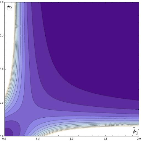
Figure 1: A contour plot of the scalar potential for a type II model of Section 3, taking all fields as real and $X,\phi_{1}$ and $\widetilde{\phi}_{1}$ in terms of $\phi_{2}$ and $\widetilde{\phi}_{2}$ according to eq.(68). Darker regions correspond to lower values of the scalar potential. At the origin one can see a non-supersymmetric vacum and far from the origin a runaway valley.

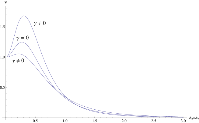
Figure 2: A 2-dimensional plot of the type II scalar potential for $\phi_{2}=\tilde{\phi}_{2}$. The parameter $\gamma$ controls R-symmetry breaking ($\gamma=0$ corresponds to the R-symmetric case). We have set $\eta=1$, and guaranteed stability in all directions of $\phi$-field space.

We shall now illustrate the results above concerning runaway directions and valleys by studying a specific example. We consider a $N_{\phi}=2$ type II model in the non-singlet case, defined by the superpotential

$$W_{SU(5)}=fX+(aX+b)\phi_{1}\widetilde{\phi}_{1}+\lambda X(\phi_{1}\widetilde{\phi}_{2}+\widetilde{\phi}_{1}\phi_{2})=\eta x+(\gamma x+1)\phi_{1}\widetilde{\phi}_{1}+x(\phi_{1}\widetilde{\phi}_{2}+\widetilde{\phi}_{1}\phi_{2})\ .$$ (64)

As before we have defined $x\equiv\lambda X/b\ ,\ \gamma\equiv a/\lambda$ and $\eta\equiv f/\lambda$; for definiteness we have set $b=1$. If one assigns the following R-charges $R(x)=2\ ,\ R(\phi_{1})=R(\widetilde{\phi}_{1})=1\ ,\ R(\phi_{2})=R(\widetilde{\phi}_{2})=-1$ then parameter $\gamma$ will control R symmetry breaking, with $\gamma=0$ corresponding to the R-symmetric case.

The scalar potential reads (with the $SU(5)$ indices omitted),

$$V_{SU(5)} = |1+\gamma\phi_{1}\widetilde{\phi}_{1}+\widetilde{\phi}_{1}\phi_{2}+\phi_{1}\widetilde{\phi}_{2}|^{2}+|(\gamma x+1)\widetilde{\phi}_{1}+x\widetilde{\phi}_{2}|^{2}$$ (65)

$$\ +|(\gamma x+1)\phi_{1}+x\phi_{2}|^{2}+|x\phi_{1}|^{2}+|x\widetilde{\phi}_{1}|^{2}\ .$$

Let us consider for definiteness a fixed direction in field space, such that only the first component in each multiplet is non-vanishing

$$\phi^{c}_{i}=\phi_{i}(1,0,\dots,0)\ ,\ \ \ \widetilde{\phi}^{\bar{c}}_{i}=\widetilde{\phi}_{i}(1,0,\dots,0)\ ,$$ (66)

where we have made explicit the $SU(5)$ indices $c,\bar{c}$. Along this direction the potential slopes to zero through directions parameterized by $\widetilde{\phi}_{2}\to\infty$, $\phi_{2}\to\infty$

$$(x,\phi_{1},\widetilde{\phi}_{1})\sim\left(\frac{1}{2\phi_{2}\widetilde{\phi}_{2}},-\frac{1}{2\widetilde{\phi}_{2}},-\frac{1}{2\phi_{2}}\right)\ .$$ (67)

Notice that the direction in field space defined by $\widetilde{\phi}_{2}=h\phi_{2}$ is a runaway direction for any value of a constant $h\neq 0$ and then one has a continuous set of runaway directions. We sketch in figure 1 the level curves of this runaway valley, in the following direction in field space

$$(x,\phi_{1},\widetilde{\phi}_{1})=\left(\frac{5}{1+5\phi_{2}\widetilde{\phi}_{2}},-\frac{\phi_{2}}{1+2\phi_{2}\widetilde{\phi}_{2}},-\frac{\widetilde{\phi}_{2}}{1+2\phi_{2}\widetilde{\phi}_{2}}\right)\ .$$ (68)

The metastable SUSY breaking vacua lies at the origin, where the boson mass-squared matrix reads

$$m_{B}^{2}=|b|^{2}\left(\begin{matrix}|\gamma x+1|^{2}+|x|^{2}&(\bar{\gamma}\bar{x}+1)x&\bar{y}\bar{\gamma}&\bar{y}\\ (\gamma x+1)\bar{x}&|x|^{2}&\bar{y}&0\\ y\gamma&y&|\gamma x+1|^{2}+|x|^{2}&(\gamma x+1)\bar{x}\\ y&0&(\bar{\gamma}\bar{x}+1)x&|x|^{2}\end{matrix}\right)\ ,$$ (69)

where we have defined $y\equiv\lambda f/|b|^{2}$. In the limit of small $y$, for some $x>x_{min}$ the eigenvalues are all positive in some range of $|\gamma|$. We plot in figure 2 the potential $V_{SU(5)}$ along the curve $\phi_{2}=\widetilde{\phi}_{2}$, which connects the metastable vacua with a runaway direction for different values of $\gamma$. For all these values, we have guaranteed stability in all directions of field space. The figure shows how changing $\gamma$ modifies the well’s depth and hence the lifetime of the metastable vacua. Our results suggest that with an appropriate choice of the R-symmetry breaking parameter one can increase the lifetime of the metastable vacua (confront this with the case of generic models, where explicit R-symmetry breaking generically induces SUSY vacua lowering the lifetime of the metastable state). Of course, in order to determine the non supersymmetric vacua’s life-time one should study quantum corrections, in the line of refs. [31]-[32]. Work on this issue is in progress [33].

4 Gauge mediating the supersymmetry breaking

In this section we turn on the gauge dynamics so that the non-singlet $\phi,\widetilde{\phi}$ messengers can interact through loops with the MSSM fields. Concerning the singlet spurion field $X$, it should acquire a non-vanishing F-component triggering SUSY breaking

$$X=X+\theta^{2}F\ .$$ (70)

The VEV of $X$ then gives mass to the messenger fields through Yukawa-like superpotential terms

$$W_{mess}={\cal M}(X)_{ij}\phi_{i}\widetilde{\phi}_{j}\ .$$ (71)

Supersymmetry breaking will then be communicated to the MSSM through gauge interactions between $\phi,\widetilde{\phi}$ and the MSSM particles. The scenario we have just described corresponds to the mechanism for gauge mediation of supersymmetry breaking (for details see for example [13]).

There are many possible ways in which the spurion $X$ develops the VEV (70). In previous sections we considered the simplest case, by adding a $fX$ term to the messenger superpotential. Of course the addition of more complicated terms can also be considered, but it will not be necessary for the analysis that follows to specify one in particular, since we will only assume that eq.(70) holds and focus on the messenger sector (71).

Some extensions of minimal or ordinary gauge mediation (OGM) were considered in [20], with the messenger superpotential containing all renormalizable couplings consistent with the Standard Model gauge invariance, renormalizability, and with a (spontaneously broken) R-symmetry, leading to a framework which was called “extra-ordinary gauge mediation” (EOGM). In this section we shall adopt the same strategy but in the case in which R-symmetry is broken explicitly in the way discussed in section 3. Following the route of [20], we will show that the explicit R-symmetry breaking terms included in the messenger sector do not in general modify the conclusions about the phenomenology of EOGM. Minimal gauge mediation with superpotentials which are deformed by mass terms were considered previously in [5]-[9], [34]-[38].

4.1 Soft masses and effective messenger number

An important property of some R-symmetric models is that the determinant of the messenger mass matrix $\cal M$ is a monomial in $X$ [20]. One can prove that this feature remains valid in type I, II and III models with explicit breaking of R-symmetry, where

$$\det{\cal M}=X^{n}G(M,L)\ ,\ \ \ \ \ \ n=\left\{\begin{matrix}\!\!\!\!\!0\ \ \ \ \ \ \ \ \ \ \ \ \ \ \ \ \ \ \ \ \ \ \ \ \ \ \ \ \ \ \ \ \ \ \ \ \ \ \ \rm Type\ I\\ \!\!N_{\phi}\ \ \ \ \ \ \ \ \ \ \ \ \ \ \ \ \ \ \ \ \ \ \ \ \ \ \ \ \ \ \ \ \ \ \ \ \ \rm Type\ II\\ \sum_{i=1}^{N_{R}}n_{i}(N_{L}(i)-N_{L}(i-1))\ \ \ \ \ \rm Type\ III\end{matrix}\right.\ .$$ (72)

We give the proof of this result in the Appendix.

The computation of gaugino and sfermion masses can be performed generalizing the wavefunction renormalization technique [39]. Concerning gaugino masses, holomorphy allows to substitute the VEV of the lowest component of $X$ by the $X$ superfield itself in the running coupling constant and renormalized wave-function. In R-symmetric models, R-symmetry is invoked to justify the analytical continuation $X\to\sqrt{X\bar{X}}$ in the sfermion mass computation. We shall proceed in the same way in the present case considering that the explicit R-symmetry breaking represents just a small correction.

In this way, ignoring effects due to multiple messenger scales, one finds for the gaugino and sfermion soft masses at the messenger scale $M_{mess}$ to order ${\cal O}(F/M_{mess}^{2})$ [20]

$$\tilde{M}_{r} = \frac{\alpha_{r}}{4\pi}\ \Lambda_{G}\ ,\ \ \ \ \ \ \ \ \ \ \ \ \ \ \ \ \ \ \ \ \ \Lambda_{G}=F\partial_{X}\log{\det\cal M}=\frac{nF}{X}\ ,$$ (73)

$$m_{\tilde{f}}^{2} = 2\sum_{r=1}^{3}C_{\tilde{f}}^{r}\left(\frac{\alpha_{r}}{4\pi}\right)^{2}\ \Lambda_{S}^{2}\ ,\ \ \ \ \ \Lambda_{S}^{2}=\frac{1}{2}F\bar{F}\frac{\partial^{2}}{\partial X\partial\bar{X}}\sum_{i=1}^{N}(\log|{\cal M}_{i}|^{2})^{2}\ .$$ (74)

Here ${\cal M}$ is the messenger mass matrix, ${\cal M}_{i}$ are messenger masses, $C_{\tilde{f}}^{r}$ are the quadratic Casimir of $\tilde{f}$ in the gauge group $r$, and ${\alpha_{r}}$ are the messenger coupling constants.

In ordinary gauge mediation models the ratio $\Lambda_{G}^{2}/\Lambda_{S}^{2}$ coincides with the number of messengers $N_{\phi}$. This fact constraints the relation between gaugino and sfermion masses, which is determined by the coupling constant. This is no more valid in EOGM [20] nor in our non-R-symmetric extension, where the ratio defines an $X$-dependent effective messenger number $N_{eff}(X)$

$$N_{eff}({\cal M}(X))\equiv\frac{\Lambda_{G}^{2}}{\Lambda_{S}^{2}}\ ,$$ (75)

taking values between $0\leq N_{eff}\leq N_{\phi}$. For asymptotic values $X\to 0$ and $X\to\infty$, the effective messenger number $N_{eff}$ becomes independent of all the parameters in $A$, $B$, $L$ and $M$, and satisfies (see Appendix)

$$\frac{n^{2}}{n^{2}-(N-r_{m}-1)(2n-N+r_{m})}\leq N_{eff}(X\to 0) \leq N-r_{m}$$ (76)

$$\frac{n^{2}}{r_{\lambda}+(r_{\lambda}-n)^{2}}\leq N_{eff}(X\to\infty) \leq\frac{n^{2}}{r_{\lambda}+\frac{(r_{\lambda}-n)^{2}}{N-r_{\lambda}}}\ ,$$ (77)

where we have defined

$$r_{\lambda}\equiv{\rm rank}\ (A+L)\ ,\ \ \ \ r_{m}\equiv{\rm rank}\ (B+M)\ .$$ (78)

In the most general case in which all possible parameters are indeed non-zero, the effective messenger number behaves asymptotically as

$$N_{eff}(X\to 0)=\left\{\begin{matrix}\!\!\!\!\!\!\!\!\!\!\!0\ \ \ \ \ \ \rm Type\ I\\ 1\ \ \ \ \ \ \rm Type\ II,III\end{matrix}\right.\ \ \ ,\ \ \ \ \ \ \ \ \ N_{eff}(X\to\infty)=\left\{\begin{matrix}\ \ \ \ \ \ \ \ 0\ \ \ \ \ \ \ \ \ \ \ \ \ \ \ \rm Type\ I\\ \ \ \ \ \ \ \ \ N_{\phi}\ \ \ \ \ \ \ \ \ \ \ \ \ \ \rm Type\ II\\ \frac{n^{2}}{N_{\phi}-1+(N_{\phi}-1-n)^{2}}\ \ \ \ \ \rm Type\ III\end{matrix}\right.\ .$$ (79)

One can infer from a specific example discussed in section 4.4 that in the whole $X$-range and in the R-symmetric case, the $N_{eff}$ range for type II models is $1-\delta\leq N_{eff}\leq N_{\phi}$ where $\delta\ll 1$, while for type III one has $n^{2}/(N_{\phi}-1+(N_{\phi}-1-n)^{2})<N_{eff}\leq 1$. When R-symmetry is broken these ranges can be extended. This is an interesting possibility since the relation between gaugino and sfermion masses crucially depend on $N_{eff}$. Moreover, when doublet/triplet splitting is considered, sleptons could be taken to be lighter than squarks. Finally, note that for type III models one can have $N_{eff}<1$, this opening the possibility of light gauginos (which takes place for $N_{eff}\ll 1$), a fact that has interesting phenomenological consequences [20].

4.2 Doublet/triplet splitting and unification

Consider the superpotential with $SU(2)$ ($2\oplus\bar{2}$) doublets $\ell,\widetilde{\ell}$ and $SU(3)$ ($3\oplus\bar{3}$) triplets $q,\widetilde{q}$

$$W={\cal M}^{(2)}_{ij}(X)\ell_{i}\widetilde{\ell}_{j}+{\cal M}^{(3)}_{ij}(X)q_{i}\widetilde{q}_{j}\ .$$ (80)

If we assume that doublets and triplets have the same R-charge assignments, then equation (72) holds for ${\cal M}^{(2)}$ and ${\cal M}^{(3)}$ with the same number $n$. As a consequence, equation (73) implies that the relations between gaugino masses are preserved, independently of the amount of doublet/tripplet splitting

$$M_{1}:M_{2}:M_{3}=\alpha_{1}:\alpha_{2}:\alpha_{3}\ .$$ (81)

We then conclude that such relations, that were believed to be valid only for models with spontaneously broken $R$-symmetry, also hold in these cases of explicit R-symmetry breaking. Since, as we shall see, unification of the coupling constants at the GUT scale can be achieved in our models, eq.(81) shows that also gaugino mass unification takes place.

The splitting we are considering also accounts for the sfermion masses (74) for which ${\Lambda_{S}^{2}}\to{\Lambda_{S}^{2}}_{r}$ with

$${\Lambda_{S}^{2}}_{r}=\Lambda_{G}^{2}{N_{eff}^{(r)}}^{-1}\ ,\ \ \ \ r=2,3\ .$$ (82)

Here ${\Lambda_{S}^{2}}_{1}=\frac{2}{5}{\Lambda_{S}^{2}}_{3}+\frac{3}{5}{\Lambda_{S}^{2}}_{2}$, and we have defined ${N_{eff}^{(r)}}\equiv N_{eff}({\cal M}^{(r)}(X))$. This shows that slepton and squark masses (74) are not only tied to the gauge couplings $\alpha_{r}$, but also to the effective messenger number ${N_{eff}^{(r)}}$, thus leading to sfermion masses which are highly modified with respect to the result of ordinary gauge mediation. This effect can lead to small mass term $\mu$ and explain the little hierarchy problem [20]. Equation (82) also receives contributions from the (non positive definite) hypercharge D-terms $D_{Y}=g_{Y}(\phi^{\dagger}Y_{\phi}\phi-\widetilde{\phi}^{T}Y_{\phi}\bar{\phi}^{*})$ which can drive slepton masses to become tachyonic. To avoid this problem one can impose on the model the messenger parity [36]-[37]

$$\phi\to U^{*}\widetilde{\phi}^{*}\ ,\ \ \ \ \widetilde{\phi}\to\widetilde{U}\phi^{*}\ ,\ \ \ \ V\to-V\ ,$$ (83)

where $V$ stands for the gauge superfields and $U$ and $\widetilde{U}$ are some unitary $N_{\phi}\times N_{\phi}$ matrices. This is a symmetry of the Lagrangian provided the following conditions on the messenger mass matrices hold

$${\cal M}^{\dagger}=U^{\dagger}{\cal M}\widetilde{U}\ ,\ \ \ \ \ ((L+A)F)^{\dagger}=U^{\dagger}(L+A)F\widetilde{U}\ .$$ (84)

Finally we notice that the splitting will also account for different running of the coupling constants. Integrating the RG equations from the ultraviolet scale $\Lambda$ down to the scale $\mu$ below the lowest messenger scale gives

$$\alpha_{r}^{-1}(\mu)=\alpha_{r}^{-1}(\Lambda)+\frac{b_{r}-N_{\phi}}{2\pi}\log\frac{\mu}{\Lambda}-\frac{1}{2\pi}\log\det\frac{{\cal M}^{(r)}}{\mu}\ ,$$ (85)

where $b_{r}=(-33/5,-1,3)$ are the MSSM $\beta$-functions. If the ultraviolet scale is the GUT scale $\Lambda=m_{GUT}$ one finds at the electroweak scale $\mu=m_{Z}$ the following relation

$$\alpha_{r}^{-1}(m_{GUT})=\alpha_{r}^{-1}(m_{Z})+\frac{b_{r}}{2\pi}\log\left(\frac{m_{GUT}}{m_{Z}}\right)-\frac{N_{\phi}}{2\pi}\log\left(\frac{m_{GUT}}{\bar{\cal M}^{(r)}}\right)\ ,$$ (86)

where we have defined $\bar{\cal M}^{(2,3)}\equiv(\det{\cal M}^{(2,3)})^{1/N\phi}$, and $\bar{\cal M}^{(1)}\equiv{\bar{\cal M}^{(2)\ 3/5}}{\bar{\cal M}^{(3)\ 2/5}}$. When $\bar{\cal M}^{(2)}=\bar{\cal M}^{(3)}$ unification is achieved at 1-loop as in the MSSM, provided the last term in (86) vanishes and the first two terms correspond precisely to the values of the MSSM couplings at the GUT scale. The challenge is to achieve arbitrary amount of doublet/triplet splitting ${\cal M}^{(2)}\neq{\cal M}^{(3)}$ without spoiling unification (i.e., maintaining $\bar{\cal M}^{(2)}=\bar{\cal M}^{(3)}$). In the R-symmetric case, this is possible since the determinants of ${\cal M}^{(r)}$ are, in general, independent of some subset of the parameters of the matrices ${\cal M}^{(r)}$. This subset can be bigger when R-symmetry is explicitly broken, and moreover, the splitting can be produced exclusively by R-symmetry breaking terms.

The relation $\bar{\cal M}^{(2)}=\bar{\cal M}^{(3)}$ implies that both $SU(2)$ and $SU(3)$ sectors belong to the same type of models (I, II, or III). In this case, the limits in which we found runaway valleys or SUSY vacua (in the case in which the superpotential was minimally completed with a $fX$ term, as in the previous section) still hold for the complete model. Suppose on the contrary that, for example, the $SU(2)$ sector is type I, and the $SU(3)$ sector is type II so that $(\det M^{(2)})^{1/N_{\phi}}=\bar{\cal M}^{(2)}\neq\bar{\cal M}^{(3)}=X(\det L^{(3)})^{1/N_{\phi}}$. In this other case, there are neither SUSY vacua nor runaway directions. The former is clear since type I and II models have no SUSY vacua, while the latter holds because type I and type II models have opposite ($X\to 0$ and $X\to\infty$ respectively) runaway directions and hence the potential slopes down to zero in one sector while the other one tends to a non zero value.

4.3 A comment on CP violating phases

As it is well-known, sources of explicit CP violation can be introduced in the MSSM through complex soft SUSY breaking terms. One should then make sure that all the constants in the hidden sector can be taken to be real by some re-phasing of fields, or otherwise the phases of the couplings should be fine-tuned. Implementing this condition together with that arising from messenger parity (83)-(84) in the R-symmetric case highly restricts the form of the messenger sector (which has to be necessarily fine-tuned), and such restriction is strengthen when R-symmetry breaking terms are added since the messenger matrix $\cal M$ can have far more entries to control.

Let us illustrate this difficulty with a simple example. Consider type II models, first in the case in which parameters are chosen so that R symmetry is not broken and the messenger superpotential reads

$$W_{mess}=\lambda X\sum_{i=1}^{N_{\phi}}\phi_{N_{\phi}-i+1}\widetilde{\phi}_{i}+m\sum_{i=1}^{N_{\phi}-1}\phi_{N_{\phi}-i}\widetilde{\phi}_{i}\ .$$ (87)

Let us define field and parameter phases as

$$\varphi_{\lambda X}\equiv-{\rm phase}(\lambda X)\ ,\ \ \ \varphi_{m}\equiv-{\rm phase}(m)\ ,\ \ \ \varphi_{i}\equiv{\rm phase}(\phi_{i})\ ,\ \ \ \widetilde{\varphi}_{i}\equiv{\rm phase}(\widetilde{\phi}_{i})$$ (88)

Re-phasing the fields and setting the parameter phases to zero leads to a solvable linear system of $2N_{\phi}-1$ equations for $2N_{\phi}$ unknowns

$$\left(\begin{matrix}1&-1&&&&&&\\ &1&-1&&&&&\\ &&&&&&&\\ &&&&&\dots&&\\ &&&&&&&\\ &&&&&&1&-1\end{matrix}\right)\left(\begin{matrix}\varphi_{1}\\ \varphi_{2}\\ \\ \vdots\\ \\ \varphi_{N_{\phi}}\end{matrix}\right)=\left(\begin{matrix}\varphi_{m}-\varphi_{\lambda X}\\ \varphi_{m}-\varphi_{\lambda X}\\ \\ \vdots\\ \\ \varphi_{m}-\varphi_{\lambda X}\end{matrix}\right)$$

$$\widetilde{\varphi}_{i}=\varphi_{\lambda X}-\varphi_{N_{\phi}-i+1}\ \,,\;\;\;\;\;\;i=1,\ldots,N_{\phi}\ .$$ (89)

Notice that this was only possible since there are only two constants $\lambda$ and $m$, and this particular form of the superpotential is not enforced by symmetries. Now, there are two different types of R-breaking terms that we can add to the hidden sector of these models

• Terms of the form

  $$\Delta W^{\not R}_{mess}=\gamma\ X\ \phi_{N_{\phi}-i_{0}}\widetilde{\phi}_{i_{0}}\ ,$$ (90)

which can only be added if $\varphi_{m}=-{\rm phase}(\gamma X)$, so that one can make $\gamma$ real.

• Terms of the form ($\gamma$ may or may not be proportional to $X$)

  $$\Delta W^{\not R}_{mess}=\gamma\phi_{i_{0}}\widetilde{\phi}_{j_{0}}\ ,\ \ \ \ \ \ \ \ 1\leq i_{0}\leq N_{\phi}-2\ ,\ \ \ 1\leq j_{0}\leq N_{\phi}-i_{0}-1\ .$$ (91)

In this case, defining $\varphi_{\gamma}=-{\rm phase}(\gamma)$ we have to add the following equation to the system (89)

$$\varphi_{i_{0}}-\varphi_{N_{\phi}-j_{0}+1}=\varphi_{\gamma}-\varphi_{\lambda X}\ ,$$ (92)

and in this case the complete system (89),(92) is solvable only for the following values of fine-tuned phases

$$(N_{\phi}-j_{0}-i_{0}+1)(\varphi_{m}-\varphi_{\lambda X})=\varphi_{\gamma}-\varphi_{\lambda X}\ .$$ (93)

We then see that in the two cases one has to fine-tune phases of coupling constants so that they can be taken as real. Once reality is imposed, eq.(84) can be satisfied (due to the fact that all $\lambda$’s and $m$’s are taken equal), and the matrices $U$ and $\widetilde{U}$ will depend on the added terms. In [40] the problem of obtaining messenger parity as an accidental symmetry is addressed.

4.4 Explicit examples of type II and III models

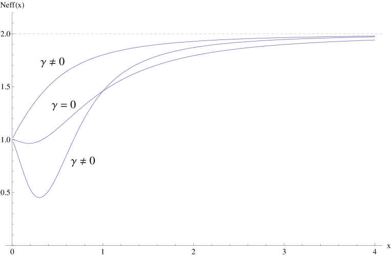
Figure 3: A plot of $N_{eff}(x)$ for different values of the R-breaking parameter $\gamma$ in a type II model.

As announced, we present here some explicit examples of gauge mediation clarifying the previously discussed features. We will not consider type I models since, as already pointed, lead to zero gaugino masses to lower order in $F/M_{mess}^{2}$ (Almost all gauge mediation models in the literature in which the hidden sector is an O’Raifeartaigh-like model correspond to this type [7]-[9], [34]-[35], [41]-[52]). Instead, we will explore type II and III models where, as we have seen, gauginos are massive. Let us start by considering the messenger sector of the type II example considered in section 3.1, with 2 messengers and superpotential

$$W_{mess}=(aX+b)\phi_{1}\widetilde{\phi}_{1}+\lambda X(\phi_{1}\widetilde{\phi}_{2}+\widetilde{\phi}_{1}\phi_{2})=(\gamma x+1)\phi_{1}\widetilde{\phi}_{1}+x(\phi_{1}\widetilde{\phi}_{2}+\widetilde{\phi}_{1}\phi_{2})\ .$$ (94)

As before we have defined $x\equiv\lambda X/b\ ,\ \gamma\equiv a/\lambda$, and set $b=1$. Being R symmetry broken, R charge assignment is arbitrary, and for definiteness we chose

$$R(x)=2\ ,\ R(\phi_{1})=R(\widetilde{\phi}_{1})=1\ ,\ R(\phi_{2})=R(\widetilde{\phi}_{2})=-1\ .$$

It is then clear that when $\gamma=0$, the theory is R-symmetric. Then, $\gamma$ will be taken as the parameter measuring the amount of R symmetry breaking.

As we have seen, at the classical level there are non-supersymmetric vacua at $\phi=\widetilde{\phi}=0\ ,\ \forall\ X$, and a runaway valley at $X\to 0$. Computing the one loop quantum correction to the moduli space one should see that, as in the R-symmetric case, the $X$ field acquires a VEV away from the origin ($X\neq 0\Rightarrow x=(\lambda X/b)\neq 0$), at least for small $\gamma$ deformation.

The effective messenger number has two interesting limits which are independent of $\gamma$

$$\lim_{x\to 0}N_{eff}(x)=1\ ,\ \ \ \ \lim_{x\to\infty}N_{eff}(x)=2\ .$$ (95)

However, the actual profile of $N_{eff}=N_{eff}(x)$ depends on $\gamma$ as can be seen in figure 3. $N_{eff}$ can take, in a certain $x$-range and for some values of $\gamma$, values below $N_{eff}<1$. Such enhancement in the range of values that $N_{eff}(x)$ can take implies that the difference between the effective numbers of the $SU(2)$ and $SU(3)$ sectors can be larger than that resulting in the R-symmetric case. Indeed, here one can have for certain values $x_{2}$ and $x_{3}$ that $|N_{eff}^{(2)}(x_{2})-N_{eff}^{(3)}(x_{3})|>1$, in which case the slepton mass could be in principle larger than the squark mass.

Now we turn to the study of the flow of the coupling constants, considering doublet/triplet splitting in the messenger sector by taking different mass matrices for $SU(2)$ and $SU(3)$. As explained in section 4.2, R-symmetry can be broken differently in each sector if $\gamma_{2}\neq\gamma_{3}$ but unification can be achieved when $\lambda_{2}=\lambda_{3}$, independently of the values of $\gamma_{i}$. We plot in figure 4 the running of the couplings for non-zero values of $\gamma_{2}$, $\gamma_{3}$, and take the masses of the messengers between $200$Tev and $5200$Tev. We see that unification takes place at the same scale as for the MSSM model with a lower value of the unified coupling constant (the same as in models with spontaneously broken R symmetry [20]).

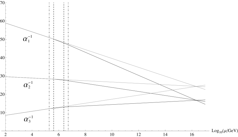
Figure 4: The running of coupling constants is plotted both when the hidden sector is present (darker full lines) and when it is absent (lighter full lines). Vertical lines indicate the mass scales of the hidden sector. Dashed and dot-dashed lines correspond to the $SU(2)$ and $SU(3)$ sector in a two messenger model.

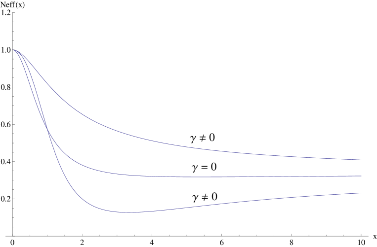
Figure 5: A $N_{eff}(x)$ for different values of the R-symmetry breaking parameter $\gamma$ in a type III model. Asymptotically all three curves tend to $N_{eff}(\infty)=2/5$.

Let us end this section by discussing the simplest example of a type III model, with $N_{\phi}=3$ messengers, defined by the superpotential

$$W_{mess}=\lambda^{\prime}X\phi_{1}\widetilde{\phi}_{3}+m\phi_{2}\widetilde{\phi}_{2}+m\phi_{3}\widetilde{\phi}_{1}+(aX+b)\phi_{2}\widetilde{\phi}_{1}=x\phi_{1}\widetilde{\phi}_{3}+\phi_{2}\widetilde{\phi}_{2}+\phi_{3}\widetilde{\phi}_{1}+(x+\gamma)\phi_{2}\widetilde{\phi}_{1}\ .$$ (96)

where we have defined $\gamma\equiv b/m$ and $x\equiv\lambda^{\prime}X/m$, and set $a=\lambda^{\prime}$ and $m=1$.

All calculations are analogous to those described in detail for the type II case. As can be seen in figure 5 the $\lim_{x\to 0}N_{eff}(x)=1$, thus coinciding with the type II behavior. In contrast, $\lim_{x\to\infty}N_{eff}(x)<1$, while in the type II case $\lim_{x\to\infty}N_{eff}(x)>1$. As in the type II model, we achieve here a spread $|N_{eff}^{(2)}(x_{2})-N_{eff}^{(3)}(x_{3})|$ that in the R-symmetric requires the addition of messengers. Note that this spread is smaller than in the type II model previously analyzed. Finally, unification of coupling constants is analogous to that described for the type II model.

5 Summary and discussion

We have analyzed, in the framework of gauge mediated supersymmetry breaking, several families of O’Raifeartaigh-type models with explicit R-symmetry breaking.

First we considered the simpler case of singlet chiral fields and determined the conditions under which such (non-generic) models have SUSY vacua and runaway behavior, in addition to a classical moduli of non-supersymmetric minima which are therefore metastable. Being the models non-generic, one can have both longlived metastable vacua and explicit, not necessarily small, R-symmetry breaking. This is not the case for generic models where R-symmetry breaking implies the existence of generic SUSY vacua and then one needs a small explicit breaking in order to have longlived local minima.

In order to analyze phenomenological features of gauge mediation, we extended the analysis to the case in which the messenger fields are in non-trivial representations of $SU(5)$ so that the resulting models can be taken as candidates for the hidden sector that gauge mediate SUSY breaking to the MSSM. The study of the corresponding vacua landscape shows that some models (only type III) have SUSY vacua only in one point of field space, except when the parameters are fine-tuned, in which case there can be more than one supersymmetric vacua. All models have continuously connected runaway directions, the runaway valleys. In addition, there is a local SUSY breaking minima at the origin of messenger field space which can be longlived.

By gauging the $SU(5)$ symmetry, we were able to analyze several issues of gauge mediation, focusing on the impact of the explicit breaking of R-symmetry. Considering a doublet/triplet-split of the gauge group we found that the relations (81) between gaugino masses and coupling constants are satisfied. We then showed that unification of couplings at the GUT scale is achieved in the same way as in the MSSM, but for a different value of unified couplings. As it happens in the R-symmetric case, in order to avoid dangerous complex phases in the soft terms, we had to tune the values of the coupling constants, which in addition allows to impose a messenger parity. Finally, we presented arguments indicating that slpetons can have masses lighter than those of squarks, as a result of the R-symmetry breaking.

An interesting feature of the models we discussed is that the R-symmetry breaking terms, chosen so that no additional SUSY-vacua exists, are precisely those that preserve the phenomenological features of extraordinary gauge mediation [20]. Another issue to be pointed concerns the possibility of spontaneous R-symmetry restoration. In fact, we have seen that the non-SUSY moduli space contains a point $X=0$ in which R-symmetry is classically not broken so that it would be possible that such point could correspond to a minimum also at the quantum level.

The breaking of supersymmetry that we discussed in our paper is not dynamical. Following the proposal of refs.[28]-[29], it should be possible to retrofit the models that we constructed so that all mass scales were generated dynamically. In this respect, the procedure should be applied in such a way that the particular form of the mass-matrices (46) is imposed by the symmetries of the dynamical SUSY breaking theory. Also, following the proposal in ref. [40], it may be possible to achieve messenger parity as an accidental symmetry. We hope to return to these issues in a forthcoming work.

Appendix

 A.1 Some identities for the messenger mass matrices

Consider three (messenger mass) matrices $\Pi$, $\Omega_{U}$, and $\Omega_{D}$ appearing in the superpotential in the form $(\Pi+\Omega_{U}+\Omega_{D})_{ij}\phi_{i}\widetilde{\phi}_{j}$, with $\det\Pi\neq 0$ and satisfying the following selection rules

$$\Pi_{ij} \neq 0\ \Rightarrow\ R(\phi_{i})+R(\widetilde{\phi}_{j})=2\ ,$$ (97)

$$(\Omega_{U})_{ij} \neq 0\ \Rightarrow\ R(\phi_{i})+R(\widetilde{\phi}_{j})<2\ ,$$ (98)

$$(\Omega_{D})_{ij} \neq 0\ \Rightarrow\ R(\phi_{i})+R(\widetilde{\phi}_{j})>2.$$ (99)

We label fields so that $i<j\Rightarrow R(\phi_{i})\leq R(\phi_{j})\ ,\widetilde{R}(\phi_{i})\leq\widetilde{R}(\phi_{j})$.

There are $(n_{1},\dots,n_{N_{R}})$ fields with R-charge assignments $(r_{1},\dots,r_{N_{R}})$ and $(\widetilde{n}_{1},\dots,\widetilde{n}_{\widetilde{N}_{R}})$ fields with R-charges $(\widetilde{r}_{1},\dots,\widetilde{r}_{\widetilde{N}_{R}})$. We group them in two sets of $N_{R}$ and $\widetilde{N}_{R}$ vectors, $\phi^{(r_{i})}_{a_{i}}$ and $\widetilde{\phi}^{(\widetilde{r}_{i})}_{\widetilde{a}_{i}}$, respectively having $n_{i}$ and $\widetilde{n}_{i}$ components ($a_{i}=1,\dots,n_{i}$; $\widetilde{a}_{i}=1,\dots,\widetilde{n}_{i}$). Matrices $\Pi$, $\Omega_{U}$, and $\Omega_{D}$ can then be arranged in blocks of $n_{i}$ rows and $\widetilde{n}_{j}$ columns each labeled by R-charges, and will be denoted as $(\Pi+\Omega_{U}+\Omega_{D})^{(r_{i},\widetilde{r}_{j})}_{a_{i},\widetilde{a}_{j}}$. We will omit indices $a_{i},\widetilde{a}_{j}$ to simplify notation.

In this basis where fields are ordered by increasing R-charge, we have

$$\Pi=\left(\begin{matrix}0&&&&\Pi^{(r_{1},\widetilde{r}_{\widetilde{N}_{R}})}\\ &&&&\\ &&\dots&&\\ &&&&\\ \Pi^{(r_{N_{R}},\widetilde{r}_{1})}&&&&0\end{matrix}\right)\ .$$ (100)

Here each block must have non-zero determinant so that the condition $\det\Pi\neq 0$ holds. This in turn implies that $\widetilde{N}_{R}=N_{R}$, $\widetilde{n}_{i}=n_{N_{R}-i+1}$, $r_{i}+\widetilde{r}_{N_{R}-i+1}=2$ and the following identity

$$\det\Pi=\prod_{i=1}^{N_{R}}\det\Pi^{(r_{i},\widetilde{r}_{N_{R}-i+1})}\neq 0\ .$$ (101)

Notice that the fields must come in pairs $(\phi_{i},\widetilde{\phi}_{N_{R}-i+1})$ satisfying $R(\phi_{i})+R(\widetilde{\phi}_{N_{\phi}-i+1})=2$.

We see from equations (98) and (99) that in the adopted basis $\Omega_{U}$ and $\Omega_{D}$ take the form

$$\Omega_{U}=\left(\begin{matrix}\Omega_{U}^{(r_{1},\widetilde{r}_{1})}&\dots&\Omega_{U}^{(r_{1},\widetilde{r}_{N_{R}-1})}&0\\ \vdots&\dots&&\\ \Omega_{U}^{(r_{N_{R}-1},\widetilde{r}_{1})}&&&\\ 0&&&0\end{matrix}\right)\ ,\ \ \Omega_{D}=\left(\begin{matrix}0&&&0\\ &&&\Omega_{D}^{(r_{2},\widetilde{r}_{N_{R}})}\\ &&\dots&\vdots\\ 0&\Omega_{D}^{(r_{N_{R}},\widetilde{r}_{2})}&\dots&\Omega_{D}^{(r_{N_{R}},\widetilde{r}_{N_{R}})}\end{matrix}\right)\ .$$ (102)

It is now clear from (100),(102) that the following identities hold

$$\det(\Pi+\Omega_{U})=\det(\Pi+\Omega_{D})=\det\Pi\ ,\ \ \ \ \det(\Omega_{D})=\det(\Omega_{U})=0\ .$$ (103)

The analysis also holds in case that the two set of fields are identical, as in Section 2.

Let us now define

$$\Pi\equiv M+XL\ .$$ (104)

In general, $\det\Pi$ would be a degree $N_{\phi}$ polynomial in the variable $X$, being $N_{\phi}$ the dimension of the matrix $\Pi$. However, by restricting the matrices $M$ and $L$ we can force $\det\Pi$ to be a monomial

$$\det\Pi=X^{n}G(M,L)\ ,$$ (105)

where $n$ is some integer between $0\leq n\leq N_{\phi}$. We consider 3 cases

• $\det M\neq 0$, $L=0$. In this case $\det\Pi=\det M$ is independent of $X$, so $n=0$.

• $\det L\neq 0$, $M=0$. In this case

  $$\det\Pi=\prod_{i=1}^{N_{R}}X^{n_{i}}\det{L^{(r_{i},\widetilde{r}_{N_{R}-i+1})}}=X^{\sum_{i=1}^{N_{R}}n_{i}}\prod_{i=1}^{N_{R}}\det L^{(r_{i},\widetilde{r}_{N_{R}-i+1})}=X^{N_{\phi}}\det L\ ,$$ (106)

  so $n=N_{\phi}$.

• $M^{(r_{i},\widetilde{r}_{N_{R}-i+1})}\neq 0\Longleftrightarrow L^{(r_{i},\widetilde{r}_{N_{R}-i+1})}=0$, and also $\det(M+L)\neq 0$.

  Notice that these two facts imply

  $$\det L^{(r_{i},\widetilde{r}_{N_{R}-i+1})}\neq 0\Longleftrightarrow\det M^{(r_{i},\widetilde{r}_{N_{R}-i+1})}=0$$ (107)

  Defining $N_{L}(k)$ the number of non-zero blocks $L^{(r_{i},r_{N_{R}-i+1})}$ of the matrix $L$ ($i=1,\dots,k$), we can arrive to the conclusion that

  $$\det L^{(r_{i},\widetilde{r}_{N_{R}-i+1})}\neq 0\Longleftrightarrow N_{L}(i)-N_{L}(i-1)=1$$

  $$\det L^{(r_{i},\widetilde{r}_{N_{R}-i+1})}=0\Longleftrightarrow N_{L}(i)-N_{L}(i-1)=0$$ (108)

  In this case,

  $$\det\Pi=\prod_{i=1}^{N_{R}}\left[\det M^{(r_{i},\widetilde{r}_{N_{R}-i+1})}+X^{n_{i}}\det L^{(r_{i},\widetilde{r}_{N_{R}-i+1})}\right]$$ (109)

  Now we can use (107) and (108) to write

  $$\det\Pi = X^{n}\prod_{i=1}^{N_{R}}\left[\det M^{(r_{i},\widetilde{r}_{N_{R}-i+1})}+\det L^{(r_{i},\widetilde{r}_{N_{R}-i+1})}\right]$$

  $$= X^{n}\prod_{i=1}^{N_{R}}\det\left[M^{(r_{i},\widetilde{r}_{N_{R}-i+1})}+L^{(r_{i},\widetilde{r}_{N_{R}-i+1})}\right]$$

  Then

  $$\det\Pi = X^{n}\det(M+L)\ ,$$ (110)

  where we have defined

  $$n=\sum_{i=1}^{N_{R}}n_{i}(N_{L}(i)-N_{L}(i-1))\ .$$ (111)

  Although $M$ has dimensional entries and $L$ is adimensional, since they are non-overlapping matrices the determinant $\det(M+L)$ has well defined mass dimensions. In units in which the superpotential $[W]=[{\rm mass}]^{3}$ and fields $[\phi]=[X]=[{\rm mass}]$, we have $\det(M+L)=[{\rm mass}]^{N_{\phi}-n}$ and then both sides in (110) have dimension [mass]${}^{N_{\phi}}$.

Finally, let us notice that calling $\Omega_{U}\equiv B+AX$, and defining

$$r_{\lambda}\equiv A+L\ ,\ \ \ \ r_{m}\equiv B+M\ ,$$ (112)

we can follow [20], to derive the relations (76)-(77) for the effective messenger number $N_{eff}$ defined in (75). In order to do that we must determine the dependence of the messenger mass matrix eigenvalues with respect to the field $X$. In what follows, we take $A$ and $L$ entries to be of order ${\cal O}(\lambda)$, and $B$ and $M$ of order ${\cal O}(m)$.

For large $X$, there are $r_{\lambda}$ messengers having ${\cal O}(\lambda X)$ masses while the remaining $N_{\phi}-r_{\lambda}$ messengers have a mass scaling with smaller powers of $X$

$${\cal M}_{i}\sim X^{-n_{i}}\ ,\ \ \ \ n_{i}\geq 0\ ,\ \ \ \ \sum_{i=1}^{N_{\phi}-r_{\lambda}}n_{i}=r_{\lambda}-n\ .$$ (113)

At small $X$, $r_{m}$ messengers have masses of the order ${\cal O}(m)$, and the remaining $N_{\phi}-r_{m}$ messengers have

$${\cal M}_{i}\sim X^{n_{i}^{\prime}+1}\ ,\ \ \ \ n_{i}^{\prime}\geq 0\ ,\ \ \ \ \sum_{i=1}^{N_{\phi}-r_{m}}n_{i}^{\prime}=n-(N_{\phi}-r_{m})\ .$$ (114)

These identities imply $N-r_{m}\leq n\leq r_{\lambda}$ and

$$N_{eff}(X\to 0)=\frac{n^{2}}{\sum_{i=1}^{N-r_{m}}(n_{i}^{\prime}+1)^{2}}\ ,\ \ \ \ \ \ N_{eff}(X\to\infty)=\frac{n^{2}}{r_{\lambda}+\sum_{i=1}^{N-r_{\lambda}}n_{i}^{2}}\ .$$ (115)

Equations (113)-(115) can be combined to show that the bounds (76)-(77) hold.

A.2  Some simple examples of O’R models with singlets

Here we analyze the classical landscape of the scalar potential in some simple O’Raifeartaigh models, in order to make contact between the general results of section 2 and explicit examples. Since we have already analyzed type II models, we focus on type I and III.

Type I models

The $N_{\phi}=N_{R}=2$ case is the non-R-symmetric version of the basic O’Raifeartaigh model [19]

$$W_{(O^{\prime}R)}=\frac{a}{2}X\phi_{1}^{2}+\frac{b}{2}\phi_{1}^{2}+m\phi_{1}\phi_{2}+fX\ ,$$ (116)

where $b$ is an R-breaking parameter. This model has no SUSY vacua, and since $N_{R}=2$ there is no runaway behavior. Notice that a shift $X\to X-b/a$ leads to the original O’Raifeartaigh model, and then our results explain, in a general context, why this model has no runaway directions.

The case $N_{\phi}=N_{R}=3$ is the R-symmetry breaking version of a R-symmetric model thoroughly analyzed in [14]. We take as superpotential

$$W_{(Sh)}=\frac{a_{1}}{2}X\phi_{1}^{2}+a_{2}X\phi_{1}\phi_{2}+\frac{b_{1}}{2}\phi_{1}^{2}+b_{2}\phi_{1}\phi_{2}+m_{1}\phi_{1}\phi_{3}+\frac{m_{2}}{2}\phi_{2}^{2}+fX\ .$$ (117)

We now show how fine-tuning different set of parameters one can obtain different R-symmetric models. Note that

$${\rm Setting}\ \ a_{2}=b_{1}=b_{2}=0\ {\rm one\ must\ set} \ R(X)=R(\phi_{3})=2,\ R(\phi_{1})=0,\ R(\phi_{2})=1$$

$${\rm Setting}\ \ a_{1}=b_{1}=b_{2}=0\ {\rm one\ must\ set} \ R(X)=2,\ R(\phi_{1})=-R(\phi_{2})=-1,\ R(\phi_{3})=3\ .\$$

There is a runaway direction

$$|X|\to\infty\ ,\ \ \ \phi_{1}\!\!\! = \!\!\!\pm\sqrt{\frac{f}{\frac{a_{2}}{m_{2}}(a_{2}X+b_{2})-\frac{a_{1}}{2}}}\ ,\ \ \ \phi_{2}=\mp\frac{1}{m_{2}}\sqrt{\frac{f(a_{2}X+b_{2})^{2}}{\frac{a_{2}}{m_{2}}(a_{2}X+b_{2})-\frac{a_{1}}{2}}}\ ,$$

$$\phi_{3}\!\!\! = \!\!\!\mp\frac{1}{m_{1}}\sqrt{\frac{f}{\frac{a_{2}}{m_{2}}(a_{2}X+b_{2})-\frac{a_{1}}{2}}}\left[a_{1}X+b_{1}-\frac{1}{m_{2}}(a_{2}X+b_{2})^{2}\right]\ ,$$ (118)

which is asymptotically the same as that of the original model[14]. Along this runaway direction, the scalar potential reaches the value of the SUSY breaking vacua ($V=|f|^{2}$) at

$$X=\frac{2m_{1}^{2}m_{2}+fa_{1}m_{2}-2fa_{2}b_{2}}{2fa_{2}^{2}}=X_{R}+\frac{a_{1}m_{2}-2a_{2}b_{2}}{2a_{2}^{2}}\ .$$ (119)

Considering $a_{2}$ as a small parameter, we can make the non SUSY minimum $\phi=0$ stable near $X\sim 0$ for some range of parameters and also sufficiently long lived.

Type III models

Let us consider two $N_{\phi}=N_{R}=3$ examples. One corresponding to the superpotential

$$W=\frac{a_{1}}{2}X\phi_{1}^{2}+a_{2}X\phi_{1}\phi_{2}+\frac{b_{1}}{2}\phi_{1}^{2}+b_{2}\phi_{1}\phi_{2}+m\phi_{1}\phi_{3}+\frac{\lambda}{2}X\phi_{2}^{2}+fX\ .$$ (120)

Here, $N_{L}(N_{R})=1$ and $N_{M}(N_{R})=2$ and then there are no runaway directions. There is a SUSY vacua at

$$X=0\ ,\ \ \ \phi_{1}=0\ ,\ \ \ \phi_{2}=\mp i\sqrt{\frac{2f}{\lambda}}\ ,\ \ \ \phi_{3}=\mp i\sqrt{\frac{2fb_{2}^{2}}{\lambda m^{2}}}\ ,$$ (121)

which can be taken far from the non-SUSY $\phi=0$ minima by considering small $|\lambda|$.

The second example corresponds to a superpotential of the form

$$W=\frac{a_{1}}{2}X\phi_{1}^{2}+a_{2}X\phi_{1}\phi_{2}+\frac{b_{1}}{2}\phi_{1}^{2}+b_{2}\phi_{1}\phi_{2}+\frac{m}{2}\phi_{2}^{2}+\lambda X\phi_{1}\phi_{3}+fX\ ,$$ (122)

and $N_{L}(N_{R})=2$ and $N_{M}(N_{R})=1$. Then, it has a runaway behavior as that in Type II models,

$$X\to 0\ ,\ \ \ \phi_{1} = \pm\sqrt{\frac{fX}{b_{1}-\frac{b_{2}^{2}}{m}+\left(\frac{a_{1}}{2}-\frac{a_{2}b_{2}}{m}\right)X}}\ ,\ \ \ \phi_{2}=\mp\frac{1}{m}\sqrt{\frac{fX(a_{2}X+b_{2})^{2}}{b_{1}-\frac{b_{2}^{2}}{m}+\left(\frac{a_{1}}{2}-\frac{a_{2}b_{2}}{m}\right)X}}\ ,$$

$$\phi_{3} = \mp\frac{1}{\lambda X}\sqrt{\frac{fX}{b_{1}-\frac{b_{2}^{2}}{m}+\left(\frac{a_{1}}{2}-\frac{a_{2}b_{2}}{m}\right)X}}\left[a_{1}X+b_{1}-\frac{1}{m}(a_{2}X+b_{2})^{2}\right]\ .$$ (123)

In addition, when $X=0$, for the fine-tuned values of the couplings $b_{1}m=b_{2}^{2}$, there is a one dimensional space of SUSY vacua parameterized by $\phi^{1}$

$$\phi_{2}=-\frac{b_{2}}{m}\phi_{1}\ ,\ \ \ \phi_{3}=-\frac{1}{\lambda\phi_{1}}\left(f+\left(\frac{a_{1}}{2}-\frac{b_{2}}{m}\right)\phi_{1}^{2}\right)\ .$$ (124)

Acknowledgements: This work was partially supported by UNLP, UBA, CICBA, CONICET and ANPCYT.

References

- [1] A. E. Nelson and N. Seiberg, Nucl. Phys. B 416 (1994) 46 [arXiv:hep-ph/9309299].
- [2] K. Intriligator, N. Seiberg and D. Shih, JHEP 0604 (2006) 021 [arXiv:hep-th/0602239].
- [3] M. Dine, W. Fischler and M. Srednicki, Nucl. Phys. B 189 (1981) 575.
- [4] S. Dimopoulos and S. Raby, Nucl. Phys. B 192 (1981) 353.
- [5] M. Dine and W. Fischler, Phys. Lett. B 110 (1982) 227.
- [6] C. R. Nappi and B. A. Ovrut, Phys. Lett. B 113 (1982) 175.
- [7] M. Dine and W. Fischler, Nucl. Phys. B 204 (1982) 346.
- [8] L. Alvarez-Gaume, M. Claudson and M. B. Wise, Nucl. Phys. B 207 (1982) 96.
- [9] S. Dimopoulos and S. Raby, Nucl. Phys. B 219 (1983) 479.
- [10] M. Dine and A. E. Nelson, Phys. Rev. D 48 (1993) 1277 [arXiv:hep-ph/9303230].
- [11] M. Dine, A. E. Nelson and Y. Shirman, Phys. Rev. D 51 (1995) 1362 [arXiv:hep-ph/9408384].
- [12] M. Dine, A. E. Nelson, Y. Nir and Y. Shirman, Phys. Rev. D 53 (1996) 2658 [arXiv:hep-ph/9507378].
- [13] G. F. Giudice and R. Rattazzi, Phys. Rept. 322 (1999) 419 [arXiv:hep-ph/9801271].
- [14] D. Shih, JHEP 0802 (2008) 091 [arXiv:hep-th/0703196].
- [15] K. Intriligator, N. Seiberg and D. Shih, JHEP 0707 (2007) 017 [arXiv:hep-th/0703281].
- [16] M. Dine and J. Mason, Phys. Rev. D 77 (2008) 016005 [arXiv:hep-ph/0611312].
- [17] A. Giveon, A. Katz and Z. Komargodski, JHEP 0806 (2008) 003 [arXiv:0804.1805 [hep-th]]; A. Giveon, A. Katz, Z. Komargodski and D. Shih, JHEP 0810 (2008) 092 [arXiv:0808.2901 [hep-th]].
- [18] S. A. Abel, C. Durnford, J. Jaeckel and V. V. Khoze, JHEP 0802, 074 (2008) [arXiv:0712.1812 [hep-ph]].
- [19] L. O’Raifeartaigh, Nucl. Phys. B 96 (1975) 331.
- [20] C. Cheung, A. L. Fitzpatrick and D. Shih, JHEP 0807 (2008) 054 [arXiv:0710.3585 [hep-ph]].
- [21] S. Ray, Phys. Lett. B 642, 137 (2006) [arXiv:hep-th/0607172].
- [22] Z. Sun, arXiv:0807.4000 [hep-th].
- [23] S. R. Coleman and E. Weinberg, Phys. Rev. D 7 (1973) 1888.
- [24] H. Abe, T. Kobayashi and Y. Omura, JHEP 0711, 044 (2007) [arXiv:0708.3148 [hep-th]].
- [25] S. Ray, arXiv:0708.2200 [hep-th].
- [26] L. Ferreti, JHEP 0712, 064 (2007) [arXiv:0705.1959 [hep-th]]; AIP Conf. Proc. 957 (2007) 221 [arXiv:0710.2535 [hep-th]].
- [27] L. G. Aldrovandi and D. Marques, JHEP 0805, 022 (2008) [arXiv:0803.4163 [hep-th]].
- [28] M. Dine, J. L. Feng and E. Silverstein, Phys. Rev. D 74, 095012 (2006) [arXiv:hep-th/0608159].
- [29] M. Dine and J. D. Mason, arXiv:0712.1355 [hep-ph].
- [30] E. Witten, Nucl. Phys. B 188 (1981) 513.
- [31] A. Riotto and E. Roulet, Phys. Lett. B 377, 60 (1996) [arXiv:hep-ph/9512401].
- [32] I. Dasgupta, B. A. Dobrescu and L. Randall, Nucl. Phys. B 483 (1997) 95 [arXiv:hep-ph/9607487].
- [33] P. Fernández and F.A. Schaposnik, to be published.
- [34] K. I. Izawa, Y. Nomura, K. Tobe and T. Yanagida, Phys. Rev. D 56 (1997) 2886 [arXiv:hep-ph/9705228].
- [35] Y. Nomura and K. Tobe, Phys. Rev. D 58 (1998) 055002 [arXiv:hep-ph/9708377].
- [36] G. R. Dvali, G. F. Giudice and A. Pomarol, Nucl. Phys. B 478 (1996) 31 [arXiv:hep-ph/9603238].
- [37] S. Dimopoulos and G. F. Giudice, Phys. Lett. B 393 (1997) 72 [arXiv:hep-ph/9609344].
- [38] S. Dimopoulos, S. D. Thomas and J. D. Wells, Nucl. Phys. B 488 (1997) 39 [arXiv:hep-ph/9609434].
- [39] G. F. Giudice and R. Rattazzi, Nucl. Phys. B 511 (1998) 25 [arXiv:hep-ph/9706540].
- [40] L. M. Carpenter, M. Dine, G. Festuccia and J. D. Mason, arXiv:0805.2944 [hep-ph].
- [41] R. Kitano, Phys. Rev. D 74 (2006) 115002 [arXiv:hep-ph/0606129].
- [42] R. Kitano, Phys. Lett. B 641 (2006) 203 [arXiv:hep-ph/0607090].
- [43] R. Kitano, H. Ooguri and Y. Ookouchi, Phys. Rev. D 75 (2007) 045022 [arXiv:hep-ph/0612139].
- [44] C. Csaki, Y. Shirman and J. Terning, JHEP 0705 (2007) 099 [arXiv:hep-ph/0612241].
- [45] H. Murayama and Y. Nomura, Phys. Rev. Lett. 98 (2007) 151803 [arXiv:hep-ph/0612186].
- [46] O. Aharony and N. Seiberg, JHEP 0702 (2007) 054 [arXiv:hep-ph/0612308].
- [47] A. Amariti, L. Girardello and A. Mariotti, Fortsch. Phys. 55 (2007) 627 [arXiv:hep-th/0701121].
- [48] N. Haba and N. Maru, Phys. Rev. D 76 (2007) 115019 [arXiv:0709.2945 [hep-ph]].
- [49] S. Abel, C. Durnford, J. Jaeckel and V. V. Khoze, Phys. Lett. B 661 (2008) 201 [arXiv:0707.2958 [hep-ph]].
- [50] S. D. L. Amigo, A. E. Blechman, P. J. Fox and E. Poppitz, arXiv:0809.1112 [hep-ph].
- [51] B. K. Zur, L. Mazzucato and Y. Oz, arXiv:0807.4543 [hep-ph].
- [52] F. Q. Xu and J. M. Yang, arXiv:0712.4111 [hep-ph].