Frequency Dependent Specific Heat from Thermal Effusion in Spherical Geometry.

Abstract

We present a novel method of measuring the frequency dependent specific heat at the glass transition applied to 5-polyphenyl-4-ether. The method employs thermal waves effusing radially out from the surface of a spherical thermistor that acts as both a heat generator and thermometer. It is a merit of the method compared to planar effusion methods that the influence of the mechanical boundary conditions are analytically known. This implies that it is the longitudinal rather than the isobaric specific heat that is measured. As another merit the thermal conductivity and specific heat can be found independently. The method has highest sensitivity at a frequency where the thermal diffusion length is comparable to the radius of the heat generator. This limits in practise the frequency range to $2$–$3$ decades. An account of the $3\omega$-technique used including higher order terms in the temperature dependency of the thermistor and in the power generated is furthermore given.

I Introduction

A hallmark of the glass transition of supercooled liquids is the time dependence of physical properties — also called relaxation. This time dependence is typically seen on the timescale of the so-called Maxwell relaxation time $\tau_{M}$. $\tau_{M}$ is defined as

$$\tau_{M}=\frac{\eta_{0}}{G_{\infty}}$$ (1)

where $\eta_{0}$ is the low frequency limiting (DC) shear viscosity and $G_{\infty}$ the high frequency limiting elastic shear modulus. The relaxation is often most easily studied in the frequency domain. At high frequencies the liquid shows solid-like elastic behaviour whereas at low frequencies it shows liquid-like viscous behaviour. In general the viscoelastic stress response to oscillatoric shear strain is described by the complex dynamic shear modulus $G$ Harrison (1976). The structural relaxation is also observed in the specific heat. This has long ago been studied in the time domain as enthalpy relaxation Davies and Jones (1953), but in 1985 frequency domain studies or AC-calorimetry Birge and Nagel (1985); Christensen (1985) were introduced in the research field of supercooled liquids. Common to these methods is that they excite thermal oscillations in the sample at a cyclic frequency $\omega$. For a heat diffusivity, $D$, this frequency is associated with a characteristic heat diffusion length,

$$l_{D}=\sqrt{\frac{D}{i\omega}},$$ (2)

the magnitude of which gives the range of the excited thermal waves. When comparing $|l_{D}|$ to a given sample size, $L$, one can classify AC-calorimetry experiments as to whether the sample is thermally thin ($L\ll|l_{D}|$) or thermally thick ($L\gg|l_{D}|$). A typical value of $D$ is $0.1\text{mm}^{2}/\text{s}$ giving $|l_{D}|\approx 0.1\text{mm}$ for a frequency of $\nu=\omega/(2\pi)=1\text{Hz}$. This means that thermally thin methods are restricted to rather low frequencies Christensen (1985); Christensen and Olsen (1998) or very thin samples Huth et al. (2007); Christensen and Olsen (1998). In these methods the temperature field is homogeneous throughout the sample and the frequency dependent specific heat is derived directly. The AC-technique allows for easy corrections of the influence of heat leaks in a non-adiabatic configuration. AC-calorimetry on thermally thick samples on the other hand has the advantage of covering a large frequency span Birge and Nagel (1985); Birge (1986). In this case the temperature field is inhomogenous and what is really measured is the effusivity, $e=\sqrt{\lambda c}$, from which the specific heat is derived. The effusivity expresses the ability of the liquid to take up heat from parts of its surface and transport it away (thermal effusion). This ability is dependent on two constitutive properties, the heat conductivity, $\lambda$, and the specific heat (pr. volume), $c$. The specific heat can only be found to within a proportionality constant in effusion experiments from an (infinite) plane. However taking boundary effects into account for finite size plane heaters Moon et al. (1996); Birge et al. (1997) one may in principle find $\lambda$ and $c$ independently. The intermediate situation where the heat diffusion length is comparable to the sample thickness has been exploited in the so-called two-channel ac calorimeter Minakov et al. (2001, 2003). This fine method aims directly at an independent determination of $\lambda$ and $c$.

The specific heat entering the effusivity is widely taken as the isobaric specific heat, $c_{p}$. However recently it has been shown Christensen et al. (2007, 2008); Christensen and Dyre (2008) that in planar and spherical geometries it is rather the longitudinal specific heat, $c_{l}$, that enters. When $M_{S}$ and $M_{T}$ are the adiabatic and isothermal longitudinal moduli respectively, $c_{l}$ is related to the isochoric specific heat, $c_{V}$, by

$$c_{l}=\frac{M_{S}}{M_{T}}c_{v}.$$ (3)

In contrast, when $K_{S}$ and $K_{T}$ are the adiabatic and isothermal bulk moduli respectively, $c_{p}$ is given by

$$c_{p}=\frac{K_{S}}{K_{T}}c_{v}.$$ (4)

Now $M_{S}=K_{S}+4/3\,G$, and $M_{T}=K_{T}+4/3\,G$. This means that $c_{l}$ will differ from $c_{p}$ in the relaxation regime where the shear modulus, $G$, dynamically is different from zero, and $K_{s}$ and $K_{T}$ differ significantly.

In this work we study the frequency dependent specific heat from thermal effusion in a spherical geometry. Specific heat measurements in a spherical geometry have earlier been conducted in the thermal thin limit Christensen and Olsen (1998), but in this paper we explore the thermal thick limit.

The justification is threefold 1) We want to realize an experimental geometry in which the thermomechanical influence on the thermal effusion can be analytically calculated Christensen and Dyre (2008). 2) The spherical container of the liquid is a piezoelectric spherical shell by which it is possible to measure the adiabatic bulk modulus Christensen and Olsen (1994) on the very same sample under identical conditions. 3) The heat conductivity and specific heat can be found independently, as the introduction of a finite length scale allows for separation of the two.

We also in this paper give an account of the $3\omega$ detection technique of our variant.

II Linear Response Theory Applied to Thermal Experiments

The experimental method used in this study is an effusion method. In such methods a harmonic varying heat current, $\mathrm{Re}(Pe^{i\omega t})$, with angular frequency $\omega$ and complex amplitude $P$, is produced at a surface in contact with the liquid; this heat then “effuses” into the liquid. At the surface a corresponding harmonic temperature oscillation, $\mathrm{Re}(\delta Te^{i\omega t})$, with complex amplitude $\delta T$, is created. The current and temperature can be thought of as stimuli and response (but which is which can be interchanged at will), and the two are linearly related if the amplitudes, $|P|$ and $|\delta T|$, are small enough. Hence it is convenient to introduce the complex frequency-dependent thermal impedance of the liquid

$$Z_{\text{liq}}=\frac{\delta T}{P},$$ (5)

this impedance depends on the properties of the liquid.

The terminology thermal impedance derives naturally from the close analogy between the flow of thermal heat and the flow of electricity Carslaw and Jaeger (1959). Temperature corresponds to electric potential and heat current to electrical current. The analogy also applies to the heat conductivity which corresponds to the specific electrical conductivity, and the specific heat which corresponds to electrical capacity.

As an example the thermal impedance of a thermally thin sample is given as

$$Z_{\text{liq,thin}}=\frac{1}{i\omega cV}$$ (6)

where $V$ is the volume of the sample. Again an equation completely equivalent to the electrical correspondence between capacitance and impedance.

In the classical case of a planar heater in a thermal thick situation the thermal impedance is found to be Birge and Nagel (1985)

$$Z_{\text{liq,planar}}=\frac{1}{A\sqrt{i\omega c\lambda}}$$ (7)

where $A$ is the plate area. The lateral dimension $W$ has to be large ($W\gg|l_{D}(\omega)|$) for this formula to be exact and unfortunately correction terms that take boundary effects into account decays only slowly as ${\omega}^{-1/2}$ Birge et al. (1997).

III Thermal Effusion in Spherical Geometry

Thermal effusion is possible in a spherical geometry as well as in a planar geometry. Imagine a liquid confined between the to radii, $r_{1}$ and $r_{2}$. The imposed oscillating outward heat current, $\mathrm{Re}\left(P(r_{1})e^{i\omega t}\right)$, at radius $r_{1}$ results in a temperature oscillation, $\mathrm{Re}\left(\delta T(r_{1})e^{i\omega t}\right)$, at the same radius. The heat wave propagating out into the liquid gives rise to a coupled strain wave due to thermal expansion. The heat diffusion is thus dependent on the mechanical boundary conditions and mechanical properties of the liquid. It is widely assumed that the transport of heat in a continuum is described by the heat diffusion equation

$$i\omega\delta T=D\nabla^{2}\delta T.$$ (8)

By the same token one might take the heat diffusion constant as $D=\lambda/c_{v}$ if the surfaces at $r_{1}$ and $r_{2}$ are clamped and $D=\lambda/c_{p}$ if one of the surfaces is free to move. This common belief is not entirely correct. If shear modulus is nonvanishing compared to bulk modulus the description of heat diffusion cannot be decoupled to a bare heat diffusion equation Landau and Lifshitz (1986); Christensen et al. (2007, 2008); Christensen and Dyre (2008). Such a situation arises dynamically at frequencies where $\omega\approx\nicefrac{{1}}{{\tau_{M}}}$. The fully coupled thermomechanical equations have been discussed in detail, by some of us, in planar geometry Christensen et al. (2007) and in spherical geometry Christensen and Dyre (2008). In general the solutions are complicated but in the case of a spherical geometry where the outer radius $r_{2}$ is much larger than the thermal diffusion length, $|l_{D}(\omega)|\ll r_{2}$ the solution becomes simple. In terms of the liquid thermal impedance, $Z_{\text{liq}}$, at the inner radius, $r_{1}$, one has

$$Z_{\text{liq}}=\frac{\delta T(r_{1})}{P(r_{1})}=\frac{1}{4\pi\lambda r_{1}\left(1+\sqrt{i\omega r_{1}^{2}c_{l}/\lambda}\right)}\,,$$ (9)

It is very interesting that in this thermally thick limit, the thermal impedance is independent of the mechanical boundary conditions Christensen et al. (2008); Christensen and Dyre (2008). I.e. in the two cases of clamped or free boundary conditions mentioned before it is neither the isochoric nor the isobaric specific heat that enters the diffusion constant and the thermal impedance but the longitudinal specific heat. Since a closed spherical surface has no boundary there are no correction terms like the ones to Eq. (7) discussed above for planar plate effusion. Notice from Eq. (9) that associated with a given radius, $r_{1}$, is a characteristic heat diffusion time for the liquid

$$\tau_{l}={r_{1}}^{2}c_{l}/\lambda.$$ (10)

$c_{l}$ and hence $\tau_{l}$ may in general be complex, but when $c_{l}$ is real, the imaginary part of $Z_{\text{liq}}$ peaks at $\omega=1/\tau_{l}$.

IV $3\omega_{\text{e}}$-detection technique

The $3\omega_{\text{e}}$ detection technique we use (where the subscript $e$ indicates that it is the electrical angular frequency not the thermal) is different from other $3\omega_{\text{e}}$ techniques (e.g. Ref. Birge and Nagel (1987)) in two ways. Firstly, we include higher order terms in the temperature dependence of the thermistor used and in the power oscillations produced. Secondly, we use a direct measurement of the time dependent voltage over a voltage divider instead of a lock-in amplifier.

IV.1 The principle.

The $3\omega_{\text{e}}$-detection technique makes it possible to measure the temperature with the same electrical resistor which generates the heat and thereby know the thermal current and the temperature at the same surface. The principle is in short the following: Applying an electrical current at cyclic frequency $\omega_{\text{e}}$ through a resistor a combined constant (zero frequency) and $2\omega_{\text{e}}$ component Joule heating is produced. This gives rise to a combined temperature DC-offset and temperature oscillation at $2\omega_{\text{e}}$, the size of which depends on the thermal environment (the thermal impedance). The resistor is chosen to be temperature dependent, it is a so-called thermistor. The temperature oscillations therefore creates a perturbation of the resistance at frequency $2\omega_{\text{e}}$. The voltage across the thermistor which by Ohm’s law is the product of current and resistance thus contains a $3\omega_{\text{e}}$ (and an additional $1\omega_{\text{e}}$) component proportional to the temperature oscillations at $2\omega_{\text{e}}$. In practise one rather has a voltage source than a current source. In order to get a $3\omega_{\text{e}}$ signal the thermistor is therefore placed in series with a temperature independent preresistor as detailed in the following.

The result of the analysis is the frequency dependent thermal impedance at a frequency of $2\omega_{\text{e}}$. It is convenient to express this thermal impedance as function of the frequency of the thermal signal which we designate $\omega$ and notice that $\omega=2\omega_{\text{e}}$.

We first outline the simplest theory in order to elucidate the technique most clearly. However, to increase the signal to noise ratio it is expedient to choose a thermistor with a large temperature dependence and to choose temperature amplitudes as high as possible although within the linear regime of the liquid thermal response. This necessitates higher harmonics be taken into account. This detailed analysis is deferred to appendix A.

IV.2 A detour on the complex notation.

Complex numbers are known to be of great use in harmonic analysis of linear systems. Since the heat current is quadratic in the imposed electrical current and the whole idea of the $3\omega_{\text{e}}$-detection technique is to exploit the inherent nonlinearity introduced by the temperature dependence of the thermistor the formalism becomes a little more troubled than in pure linear applications. Thus we have to drag around the complex conjugate terms in order to get product terms right.

Generally a sum of harmonic terms,

$$A=A_{0}+|A_{1}|\cos(\omega_{\text{e}}t+\phi_{1})+\ldots+|A_{n}|\cos(n\omega_{\text{e}}t+\phi_{n}),$$ (11)

with real amplitudes, $A_{0}$,$|A_{k}|$, and phases, $\phi_{k}$, can be written as,

$$A=\frac{1}{2}\left(A_{0}+A_{0}+|A_{1}|e^{i(\omega_{\text{e}}t+\phi_{1})}+|A_{1}|e^{-i(\omega_{\text{e}}t+\phi_{1})}+\ldots\right.\\ \left.+|A_{n}|e^{i(n\omega_{\text{e}}t+\phi_{n})}+|A_{n}|e^{-i(n\omega_{\text{e}}t+\phi_{n})}\right).$$ (12)

By introducing the complex amplitudes $A_{k}=|A_{k}|e^{i\phi_{k}}$ and the shorthand notation $E_{k}=e^{ik\omega_{\text{e}}t}$ the sum becomes

$$A=\frac{1}{2}(A_{0}+A_{1}E_{1}+\ldots+A_{n}E_{n}+c.c.),$$ (13)

where $+c.c.$ means that the complex conjugated of all the terms within the parenthesis should be added, including the real constant term. Note that $E_{0}=1$, $E_{k}E_{l}=E_{k+l}$, and $E_{k}E_{l}^{*}=E_{k-l}$.

Notice that any product of an $n$’th and $m$’th harmonic will produce both an $n+m$’th and $n-m$’th harmonic term. Furthermore the DC-components get doubled because there is no difference between $E_{0}$ and $E_{0}^{*}$.

IV.3 Fundamental equations for the voltage divider

Consider the diagram of the electrical setup seen in Fig. 1. $U(t)$ is the voltage of the source and $V(t)$ the voltage across the temperature independent preresistor, $R_{\text{pre}}$. $U(t)$ and $V(t)$ can be measured directly. $R(T(t))$ is the temperature dependent resistance of the heater/sensor (we will explicitly state the temperature/time dependencies when appropriate, otherwise it is implicitly assumed).

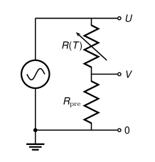
Figure 1: Voltagedivider for the $3\omega_{\text{e}}$-detection technique. The temperature-dependent resistor (the thermistor), $R(T)$, is in thermal contact with the liquid probing its thermal impedance at $2\omega_{\text{e}}$. The preresistor, $R_{\text{pre}}$, is temperature-independent.

The current $I(t)$ through $R(T(t))$ and $R_{\text{pre}}$ is given as

$$I(t) = \frac{U(t)}{R_{\text{pre}}+R(T(t))}=\frac{V(t)}{{R_{\text{pre}}}},$$ (14)

and the power produced in the heater as

$$P(t)=I(t)^{2}R(T(t))=\frac{R(T(t))}{\left(R_{\text{pre}}+R(T(t))\right)^{2}}U(t)^{2}.$$ (15)

Eq. (14) gives the voltage divider equation,

$$V(t)=\frac{R_{\text{pre}}}{R_{\text{pre}}+R(T(t))}U(t),$$ (16)

which in principle allows for determination of $T(t)$ from the measured voltages.

IV.4 The AC-method to lowest order

The thermistor and the surrounding sample are placed in a cryostat that defines an overall reference temperature, $T_{\text{cryo}}$. The power produces a (real) temperature change $\Delta T=T-T_{\text{cryo}}$ at the heater/sensor depending on the thermal impedance, $Z$, (as defined in section II) the heater/sensor looks into. The temperature rise has a real DC-component, $T_{0}$, and complex AC-components. It can in general be written as

$$\Delta T=\frac{1}{2}(T_{0}+T_{1}E_{1}+T_{2}E_{2}+T_{3}E_{3}+T_{4}E_{4}+...+c.c.)$$ (17)

the dominant terms will be the DC component, $T_{0}$, and the second harmonic term, $T_{2}$ (see next section).

To first order in the temperature variations the thermistor has a resistance of

$$R=R_{0}(1+\alpha_{1}\Delta T).$$ (18)

Here $R_{0}$ and $\alpha_{1}$ are considered constant at a given cryostate temperature but they vary with $T_{\text{cryo}}$. In fact the thermistor, which is based on a semiconducting material, has a resistance that over a larger temperature range is very well described by

$$R=R_{\infty}e^{T_{a}/T},$$ (19)

with $T_{a}$ the activation temperature and $R_{\infty}$ the infinity temperature limiting resistance. $\alpha_{1}$ is related to $T_{a}$ by

$$\alpha_{1}=\frac{1}{R(T_{\text{cryo}})}\left.\frac{dR}{dT}\right|_{T_{\text{cryo}}}=-\frac{T_{a}}{T_{\text{cryo}}^{2}}.$$ (20)

Characteristic values of $R_{\infty}$ and $T_{a}$ are given in table 1.

Table 1: Experimental parameters. Top: Parameters characterizing the resistors in the setup, $R_{\text{pre}}$ is the resistance of the preresistor, $R_{\infty}$ and $T_{a}$ the characteristics of the thermistor according to Eq.  (19)). Middle: Absolute size of the thermistor bead. Measured values indicates the eccentricity of the bead. The optimize value is the one use in the final treatment of the data, and is optimized to give best correspondence between the room temperature DC specific heat, and the literature value of this. Bottom: Applied amplitudes expressed as mean applied voltage, ($\langle|U_{1}|\rangle_{\nu}$), and maximum temperature amplitude, ($\max(|T_{2}|)_{\nu,T})$.

$R_{\text{pre}}$	$3884.3\mathrm{\SIUnitSymbolOhm}$
$R_{\infty}$	$0.1251\mathrm{\SIUnitSymbolOhm}$
$T_{a}$	$2789.5\mathrm{K}$
$r_{1,\text{Measured, long edge}}$	$0.205\mathrm{m}\mathrm{m}$
$r_{1,\text{Measured, short edge}}$	$0.185\mathrm{m}\mathrm{m}$
$r_{1,\text{Optimized}}$	$0.2073\mathrm{m}\mathrm{m}$
$\langle|U_{1}|\rangle_{\nu}$	$4.909\mathrm{V}$
$\max(|T_{2}|)_{\nu,T}$	$2.253\mathrm{K}$

Substituting Eq. (18) into Eq. (16) we obtain

$$V=\frac{1}{1+A(1+\alpha_{1}\Delta T)}U\approx\frac{1}{A+1}\left(1-a\Delta T\right)U$$ (21)

where $A=R_{0}/R_{\text{pre}}$, $a=\frac{A\alpha_{1}}{1+A}$ and the second expression is to first order in $\Delta T$ like in Eq. (18).

In the simple case, which we first discuss, we assume that the function generator can deliver a pure single harmonic voltage,

$$U(t)=\frac{1}{2}(U_{1}E_{1}+c.c).$$ (22)

Eqs. (17) and (22) can now be substituted into Eq. (21).

$$V=\frac{1}{A+1}\left(1-a\left(\frac{1}{2}(T_{0}+T_{1}E_{1}+T_{2}E_{2}+T_{3}E_{3}+\right.\right.\\ \left.\left.\vphantom{\frac{1}{2}}T_{4}E_{4}+\ldots+c.c.)\right)\right)\frac{1}{2}(U_{1}E_{1}+U_{1}^{*}E_{1}^{*}).$$ (23)

In principle the result contains all harmonics, but it turns out that the interesting ones are the first and third harmonic. The complex amplitudes are by inspection seen to be

$$V_{1}=\frac{1}{A+1}\left(U_{1}-aT_{0}U_{1}-\frac{1}{2}aT_{2}U_{1}^{*}\right)$$ (24)

and

$$V_{3}=\frac{1}{A+1}\left(-\frac{1}{2}aT_{2}U_{1}-\frac{1}{2}aT_{4}U_{1}^{*}\right).$$ (25)

Notice that even if $\Delta T$ is written as an infinite sum (as in Eq. (17)), $V_{1}$ and $V_{3}$ have only the included terms. This is a consequence of assuming a perfect voltage source.

The $T_{4}$ term can be neglected, since it is proportional to a higher order power term, $P_{4}$, which is small. This approximation leads to the a use full relationship between the $3\omega_{\text{e}}$-term and the temperature amplitude at $2\omega$, $T_{2}$,

$$V_{3}=-\frac{1}{2}\frac{a}{(A+1)}T_{2}U_{1}.$$ (26)

Eq. (24) and (26) can be solved for $T_{0}$ and $T_{2}$ if prior knowledge on the temperature dependency of the resistance of the thermistor exists, that is if $A$ and $a$ are known at the relevant temperatures. The $T_{2}$ and $T_{0}$ component terms are related to the power through the complex AC-thermal impedance, $Z_{2}$ (the impedance at $2\omega_{\text{e}}$), and DC-thermal impedance, $Z_{0}$ as

$$T_{0}=Z_{0}P_{0}\ \text{and}\ T_{2}=Z_{2}P_{2}.$$ (27)

The temperature dependency of the thermistor resistance can of course be found from calibration measurements. We have however found it to be more efficient to use an iterative solution technique eliminating the need for prior calibration. Eq. (24) and (26) are rewritten in the following form

$$A = \frac{\left(U_{1}-aT_{0}U_{1}-\frac{1}{2}aT_{2}U_{1}^{*}\right)}{V_{1}}-1$$ (28a)

$$T_{2} = -2\frac{V_{3}(A+1)}{aU_{1}}.$$ (28b)

It can be seen that the equation for $A$ consists of the $0$’th order expression $A\approx\nicefrac{{U_{1}}}{{V_{1}}}-1$ which would be valid if the temperature of the thermistor bead was the same as the cryostat temperature. This is not the case as the thermistor generates self heat, which is what the two additional terms correct for.

$A$ and $T_{2}$ can be found by iteration in the following way. A first approximation of $A$ is found by setting $T_{0}=0$ and $T_{2}=0$ in Eq. (28a). Based on this an initial estimate of $\alpha_{1}$ is found from the temperature dependence of $A$. An estimate on $T_{2}$ (and hence $Z_{2}$) is afterwards found from Eq. (28b). By extrapolating $Z_{2}$ to zero frequency an estimate of $T_{0}$ is found (utilizing $T_{0}=Z_{0}P_{0}$). The estimated values for $T_{0},T_{2}$ and $a$ can then be inserted into Eq. (28a) giving a better estimate for $A$. This iteration procedure can be repeated a number of times and converges rapidly to a fixpoint for $A$ and $T_{2}$.

IV.5 Thermal-power terms

If the 1. order approximation of the resistance of the thermistor, Eq. (18), is substituted into the power equation, Eq. (15), the following expression is obtained to first order in $\alpha_{1}\Delta T$

$$P=\frac{1}{R_{\text{pre}}}\frac{A(1+\alpha_{1}\Delta T)}{(1+A(1+\alpha_{1}\Delta T))^{2}}U^{2}\approx\\ \frac{1}{R_{\text{pre}}}\frac{A}{(1+A)^{2}}\left(1+\frac{1-A}{1+A}\alpha_{1}\Delta T\right)U^{2}.$$ (29)

This shows that an input voltage which is a pure 1. harmonic leads to dominant 0. and 2. harmonics in the power/temperature. Notice that if the thermistor resistance were temperature independent, that is $\alpha_{1}=0$, then $P_{0}$ equals $|P_{2}|$ exactly but in general they are almost identical, $P_{0}\approx|P_{2}|$.

It can further be seen that even if the voltage generator is purely single harmonic, the power can have a $4\omega_{\text{e}}$ component from the interplay between the $2\omega_{\text{e}}$ temperature variation and the $2\omega_{\text{e}}$ variation of the squared voltage. In principle further higher harmonics are generated this way. It can however be observed that if $\alpha_{1}\Delta T$ is small, or if $A\approx 1$ which can be chosen in the setup, the higher harmonics will be small (and decreasing with order).

Eq. (29) is not very practical for calculating the thermal-power terms needed for evaluating the thermal impedance from the temperature amplitudes obtained from Eq. (28), since $\Delta T$ is needed.

Alternatively the thermal power can be written as

$$P = I(U-V)=\frac{(U-V)V}{R_{\text{pre}}}$$ (30)

using Eq. (14). From this equation the power can be directly determined from measurable quantities.

If only the $1\omega_{\text{e}}$ component of the voltage is taken into account the following approximations are obtained

$$P\approx\frac{1}{4R_{\text{pre}}}((U_{1}-V_{1})E_{1}+c.c.)(V_{1}E_{1}+c.c.)=\\ \frac{1}{4R_{\text{pre}}}((U_{1}-V_{1})V_{1}^{*}+(U_{1}-V_{1})V_{1}E_{2}+c.c.)$$ (31)

leading to power coefficient given as

$$P_{0}=\frac{1}{4R_{\text{pre}}}((U_{1}-V_{1})V_{1}^{*}+(U_{1}^{*}-V_{1}^{*})V_{1})$$ (32a)

and

$$P_{2}=\frac{1}{2R_{\text{pre}}}(U_{1}-V_{1})V_{1}.$$ (32b)

A more general expansion including higher harmonics is given in appendix B.

IV.6 The AC-method refined

As mentioned earlier we have to do a refined analysis of the detected harmonics of the voltages. These extra terms stem from different sources: 1) The voltage source itself has higher harmonics and a DC-offset. 2) A second order term in the temperature dependence of the thermistor resistance. 3) The $4\omega_{\text{e}}$ Joule-power component produced by the $2\omega_{\text{e}}$ variation of the thermistor (as discussed in section IV.5). These effects are taken into account, as described below.

Regarding point 1) we write the source voltage, $U(t)$, more generally as

$$U(t)=\frac{1}{2}\left(U_{0}+U_{1}E_{1}+U_{2}E_{2}+U_{3}E_{3}+U_{4}E_{4}+c.c.\right)$$ (33)

including up to the fourth order harmonics. A $U_{3}$ component from the source is to be expected since the source itself has an inner resistance. The $U_{0}$ is a DC-offset that was present in this experiment but in principle should be eliminated.

Regarding point 2) we expand the temperature dependence of the thermistor to second order as

$$R=R_{0}(1+\alpha_{1}\Delta T(t)+\alpha_{2}\Delta T(t)^{2}).$$ (34)

Because $R(T)$ follows Eq. (19) over an extended temperature range $\alpha_{2}$ and $\alpha_{1}$ are connected as

$$\alpha_{2}=\frac{\alpha_{1}^{2}}{2}-\frac{\alpha_{1}}{T_{\text{cryo}}}.$$ (35)

Point 3) is taken into account by expanding $V(t)$, $P(t)$ and $T(t)$ like $U(t)$ in Eq. (33) up to the fourth harmonic components also.

The full analysis can be found in the appendix A, including terms larger than $5\cdot 10^{-7}U_{1}$. Fortunately it leads to rather simple extensions of the Eqs. 28

$$A = \frac{\left[U_{1}-aT_{0}U_{1}-\frac{1}{2}aT_{2}U_{1}^{*}+X_{1}\right]}{V_{1}}-1$$ (36a)

$$T_{2} = -2\frac{V_{3}(A+1)-\left(U_{3}+X_{3}\right)}{aU_{1}}.$$ (36b)

$X_{1}$ and $X_{2}$ depends on $T_{0}$, $T_{1}$, $T_{2}$, $T_{4}$, and $b=\left(\frac{A\alpha_{1}}{1+A}\right)^{2}-\frac{A\alpha_{2}}{1+A}$, and the expressions are given in Eq. (51).

The coupled Eqs. (36), can be solved by iteration, using a procedure equivalent to the one for the first order solution.

We start by estimating $A(T)$ from Eq. (36a), putting $X_{1}=T_{0}=T_{2}=0$, and from this estimate $\alpha_{1}$ and $\alpha_{2}$.

A provisory thermal impedance $Z_{2}$ is then found from Eq. (36b). $T_{1}=Z_{1}P_{1}$ and $T_{4}=Z_{4}P_{4}$ can then be estimated since $Z_{1}(\omega)=Z_{2}(\omega/2)$ and $Z_{4}(\omega)=Z_{2}(2\omega)$, and $T_{0}$ is found from the limit of $Z_{0}$ as described earlier. The perturbative terms, $X_{1},X_{3}$, can then be found and with these values in Eqs. (36a) and (36b) a better estimation of $A$ (and hence $\alpha_{1}$ and $\alpha_{2}$) and $T_{2}$ is found. This process is iterated until convergence.

The two important power components are calculated from the $V_{i}$’s and $U_{i}$’s as in Eq. (32) by

$$P_{0}=\frac{1}{R_{\text{pre}}}\left(W_{0}V_{0}+\frac{1}{2}\mathrm{Re}\left(W_{1}V_{1}^{*}+W_{2}V_{2}^{*}+W_{3}V_{3}^{*}+W_{4}V_{4}^{*}\right)\right)$$ (37)

and

$$P_{2}=\frac{1}{R_{\text{pre}}}\left(W_{0}V_{2}+W_{2}V_{0}+\vphantom{\frac{1}{2}}\right.\\ \left.\frac{1}{2}\left(W_{1}V_{1}+W_{1}^{*}V_{3}+W_{2}^{*}V_{4}+W_{3}V_{1}^{*}+W_{4}V_{2}^{*}\right)\right)$$ (38)

where $W=U-V$. The full set of power components are given in Eq. (52).

V Experimental

The measurements were performed using a custom built setup Igarashi et al. (2008a, b). The temperature was controlled by a cryostat with temperature fluctuations smaller than $2\mathrm{m}\mathrm{K}$ (see Ref. Igarashi et al., 2008a for details on the cryostat). The electrical signals were measured using a HP3458A multimeter in connection with a custom-built frequency generator as sketched on Fig. 1 (see Ref. Igarashi et al. (2008b) for details on the electrical setup, but notice that in this experiment we used the generator and multimeter in a slightly altered configuration). The electrical setup allows for measurements in the frequency ($\nu_{\text{e}}$) range from $1\mathrm{m}\mathrm{Hz}$ up to $100\mathrm{Hz}$.

The used thermistor was of the type U23UD from Bowthorpe Thermometrics, and was positioned in the middle of a sphere as shown on Fig. 2. The details of the sphere is as discussed earlier unimportant, and in this case the piezoelectric bulk transducer Christensen and Olsen (1994) is used as such. The sphere is filled at room temperature with additional liquid in the reservoir. This additional liquid ensures that the sphere stays completely filled as it is cooled to the relevant temperature.

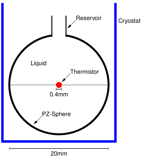
Figure 2: Schematic illustration of the measuring setup. The thermistor acting as combined heater and thermometer is placed in a sphere filled with the liquid. The sphere is itself placed in a cryostat.

The liquid investigated was a five-ring polyphenyl ether (5-polyphenyl-4-ether) the Santovac® 5 vacuum pump fluid (CAS number 2455-71-2). The liquid was used as received, without further purification.

Data were taken as frequency scans at constant temperature, with the liquid in thermal equilibrium. The direct output from the frequency generator was measured under electrical load, at each sample temperature. This eliminates any long term drifts in the frequency generator output voltage. The measurements were furthermore carried out at two different input amplitudes, $\langle|U_{1}|\rangle\approx 4.9\mathrm{V}$ and $\langle|U_{1}|\rangle\approx 2.9\mathrm{V}$, allowing for a test of the inversion algorithm and linearity of the final thermal response. If not stated otherwise all results presented in this paper are from the larger of the two amplitudes. To test for reproducibility and equilibrium some of the measurements were retaken during the reheating of the sample. The outcome of the measurements are the complex amplitudes $U_{i}(\nu_{\text{e}})$ and $V_{i}(\nu_{\text{e}})$ for the harmonics of the voltages $U$ and $V$.

Table 1 gives the key experimental parameters for the measurements at the high input amplitude.

VI Data analysis

In the following we denote the measured thermal impedance, $Z_{2}$, by simply $Z$ dropping the subscript $2$. The subscripts were practical in the technical description of the detection method indicating that the thermal impedance is found at a thermal frequency, $\omega$, which is the double of the electrical frequency, $\omega_{e}$. But in discussing the thermal properties of liquids only the thermal frequency $\omega=2\pi\nu$ is relevant. The temperature we refer to at which a measurement is done is the mean temperature at the bead surface, $T=T_{0}+T_{\text{cryo}}$.

The thermal impedance has been measured at two different input voltage amplitudes, $U_{1}$, of the voltage divider of Fig. 1 and thus at two different power amplitudes. The liquid thermal response, the temperature, is expected to be linear in the power amplitudes and thus the thermal impedance should be independent of the power amplitude.

The thermal impedance has been calculated from the measured voltage harmonics using both the first-order method described in section IV.4 and using the higher-order method described in section IV.6.

The top part of Fig. 3 shows the frequency dependent relative difference between the calculated thermal impedance from the two amplitudes. The results from the two methods (the first-order and higher-order methods) for three selected temperatures are shown in the figure. In the lower part the average relative difference is shown as function of temperature. It is seen that the higher order method generally reduces the difference significantly. Only in a very small temperature interval does the two methods give equally good results. This demonstrates the necessity of taking into account the higher-order terms of the elaborated analysis (as described in section IV.6).

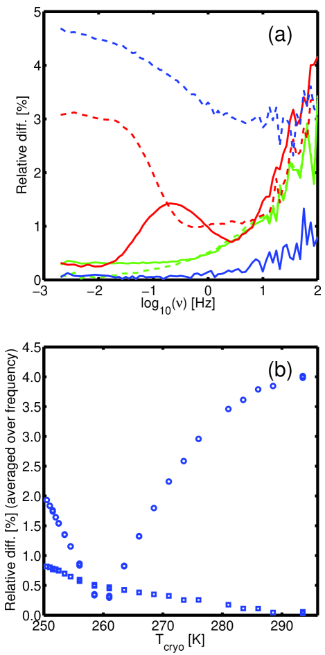
Figure 3: Comparison of the thermal impedance, $Z$, obtained from the measurements at two different amplitudes ($\langle U_{1}\rangle=4.9\mathrm{V}$ and $2.9\mathrm{V}$), and from using the first-order model as given in Eq. (28) and higher-order model as given in Eq. (36) (as described in section IV.4 and IV.6).
(A) the frequency dependent relative difference between the two methods ($|Z_{\text{amp}=2.9\mathrm{V}}-Z_{\text{amp}=4.9\mathrm{V}}|/|Z_{\text{amp}=2.9\mathrm{V}}|$). Full lines: the difference for the higher-order model. Dashed lines: the difference for the first-order model. Cryostat temperatures are $293.5\mathrm{K}$ (blue), $261\mathrm{K}$ (green) and $250.5\mathrm{K}$ (red).
(B) shows the frequency averaged relative difference ($\langle|Z_{\text{amp}=2.9\mathrm{V}}-Z_{\text{amp}=4.9\mathrm{V}}|\rangle_{\nu}/\langle|Z_{\text{amp}=2.9\mathrm{V}}|\rangle_{\nu}$). Squares the difference for the higher-order model. Circles the difference for the first-order model.

Fig. 4 shows the real and imaginary part of the thermal impedance, $Z$, in a log-log plot at $295.6\mathrm{K}$. The measured impedance has more features than predicted by the simple expression for the thermal impedance of spherical effusion Eq. (9). For example the high frequency behavior should be characterized by a line of slope $1/2$ but this is seen not to be the case. The additional features come from thermal properties of the thermistor bead, the influence of which we are going to study below. We stress that although $Z$ shows dispersion and has a real and imaginary part this has nothing to do with liquid relaxation — which is absent at this temperature — but is only a consequence of heat diffusion in spherical geometry. However relaxation should of course affect the thermal impedance. This is shown in Fig. 5 where $Z$ at $252.7\mathrm{K}$ and $256.7\mathrm{K}$ are compared. The glass transition is seen to give only a slight perturbation of the shape of the $Z$-curve. In order to obtain any reliable specific heat data from the thermal impedance it is thus imperative to have an accurate model of the thermal interaction between liquid and thermistor bead.

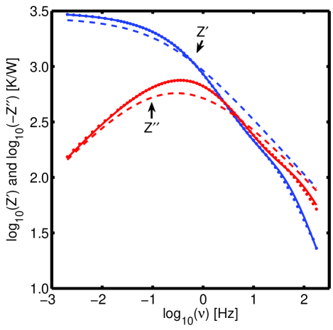
Figure 4: Comparison of measured thermal impedance, $Z$, with the result from fitting the full model of liquid and thermistor (Eqs. (9), (42) and (43)), and the simple model of $Z_{\text{liq}}$ (Eq. (54)). The parameters used in evaluation of the simple model are the ones found from the full analysis. Data are taken at room temperature ($T=295.6\mathrm{K}$). Dots: measured points. Full lines: full model of liquid and thermistor bead. Dashed lines simple model including only the liquid.

The bead (see Fig. 6) consists of a core of radius $r_{0}$, where the temperature amplitude $\delta T$ is actually measured and the heat current $P$ generated. This core is surrounded by a glass capsule of outer radius $r_{1}$, at which the bead is in contact with the liquid. The heat flow $P(r_{1})$ out through the surface at $r_{1}$ is in general different from the heat flow $P(r_{0})$ out through the surface at $r_{0}$. Also the temperature $\delta T(r_{1})$ can be different from $\delta T(r_{0})$. Now the liquid thermal impedance is

$$Z_{\text{liq}}=\frac{\delta T(r_{1})}{P(r_{1})}$$ (39)

whereas the measured thermal impedance is rather

$$Z=\frac{\delta T}{P}.$$ (40)

The capsule layer has a heat conductivity $\lambda_{b}$ and a specific heat $c_{b}$. The bead is a solid for which in general the difference between the isobaric and isochoric specific heats are small and they are frequency independent. The heat diffusion through this shell is thus well described Christensen and Dyre (2008) by a thermal transfermatrix, $\textbf{T}^{\rm th}=\textbf{T}^{\rm th}(\lambda_{b},c_{b},r_{1},r_{0})$,

$$\begin{pmatrix}\delta T(r_{1})\\ P(r_{1})/(i\omega)\end{pmatrix}\,=\,\textbf{T}^{\rm th}\begin{pmatrix}\delta T(r_{0})\\ P(r_{0})/(i\omega)\end{pmatrix}\,.$$ (41)

This implies that the thermal impedance $Z_{\text{liq}}=Z_{r_{1}}$ at radius $r_{1}$ is transformed to a thermal impedance $Z_{r_{0}}$ at radius $r_{0}$ via

$$Z_{r_{0}}=\frac{1}{i\omega}\frac{T^{\rm th}_{12}-T^{\rm th}_{22}i\omega Z_{\text{liq}}}{T^{\rm th}_{11}-T^{\rm th}_{21}i\omega Z_{\text{liq}}}.$$ (42)

A small part of generated power is stored in the core of the bead. The heat capacity $C_{\text{core}}$ of the core is taken to be $4/3\pi{r_{0}}^{3}c_{b}$. The measured thermal impedance $Z$ is thus related to $Z_{r_{0}}$ by

$$\frac{1}{Z}=i\omega C_{\text{core}}+\frac{1}{Z_{r_{0}}}$$ (43)

The model relating $Z_{\text{liq}}$ to the measured $Z$ described by Eqs. (9), (42) and (43) are depicted in the electric equivalent diagram in Fig 6.

In order to get $Z_{\text{liq}}$ from the measured $Z$ one has to know the parameters $r_{0},r_{1},\lambda_{b}$ and $c_{b}$ characterizing the thermal structure of the intervening thermistor bead.

This can in principle be done by fitting $Z$ of the model obtained by combining Eqs. (9), (42), and (43) to the measured frequency dependent thermal impedance. An electric equivalent network of the model is depicted in Fig. 6. This model has six frequency independent intrinsic parameters, namely $r_{0},r_{1},\lambda_{b},c_{b},\lambda$ and $c_{l}$, if the fit is limited to the temperature region where $c_{l}$ can be considered frequency independent. By careful inspection of the equations it can be found that the number of independent parameters that can be deduced from a fit is only five. The five parameters can be chosen in a number of ways, of which we have chosen

$$\tau_{l}=r_{1}^{2}\frac{c_{l}}{\lambda},\ \tau_{b}=r_{1}^{2}\frac{c_{b}}{\lambda_{b}},\ \hat{r}=\frac{r_{0}}{r_{1}},\quad\hat{c}=\frac{c_{l}}{c_{b}},\ Z_{\text{liq},0}=\frac{1}{4\pi\lambda r_{1}}.$$ (44)

This set of variables has the advantage that it minimizes the number of parameters which mix bead and liquid properties. Here $\hat{c}$ is the only one such mixed parameter. The expressions for the transfermatrix and $Z_{\text{liq}}$ in terms of these parameters is given in appendix C.

The five parameter model was fitted to the measured thermal impedance, $Z$, by using a least square algorithm. The results are shown on Fig. 7 and 8. Measurements were taken both going downwards to the glass transition and upwards again to room temperature. In the glass transition range where the liquid specific heat, $c_{l}$, is expected to be complex and frequency dependent these fits of course do not work. This is the reason for the scatter of data at low temperature. This difference between the high and low temperature regimes can also be seen directly in the error from the fit as illustrated on the lower part of Fig. 8.

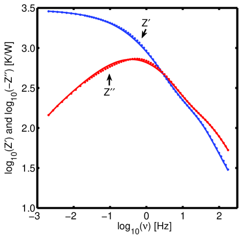
Figure 5: Comparison of thermal impedance, $Z$, at two temperatures, showing the small difference due to the frequency dependent specific heat of the liquid, $c_{l}(\nu)$. Lines: $T=256.9\mathrm{K}$. Dots $T=252.8\mathrm{K}$.

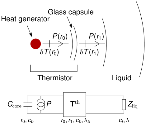
Figure 6: Schematic thermal network model of the thermistor bead and liquid. The thermal current $P$ and temperature $\delta T$ are indicated at the inner radius, $r_{0}$, at the border between the heater and the glass capsule and at the outer radius, $r_{1}$, at the border between the glass capsule and the liquid. The thermal impedance of the liquid is defined as $Z_{\text{liq}}=\delta T(r_{1})/P(r_{1})$. The thermal impedance seen from the thermistor is $Z=\delta T(r_{0})/P$. The two are connected by Eq. (42) and (43), utilizing the thermal transfermatrix Eq. (55).

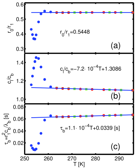
Figure 7: Results from fitting the measured thermal impedance, $Z$, to the $5$-parameter thermal network model (Fig. 6) of the spherical heat effusion experiment Eqs. (9), (42) and (43). This figure shows (a) $\hat{r}=r_{0}/r_{1}$ , (b) $\hat{c}=c_{l}/c_{b}$ and (c) $\tau_{b}$, (the remaining parameters are shown on figure 8).
Open squares (red): Data taken going down in temperature. Open circles (green): Data taken going up in temperature. Closed circles (blue): Low temperature data including points take going down and up. Line: Interpolated temperature dependencies of $\hat{r}$, $\hat{c}$ and $\tau_{b}$ found based on data from above the liquid glass transition temperature range, used for extrapolating down in the region where the liquid relaxation sets in (the functional form and fitting results are shown).

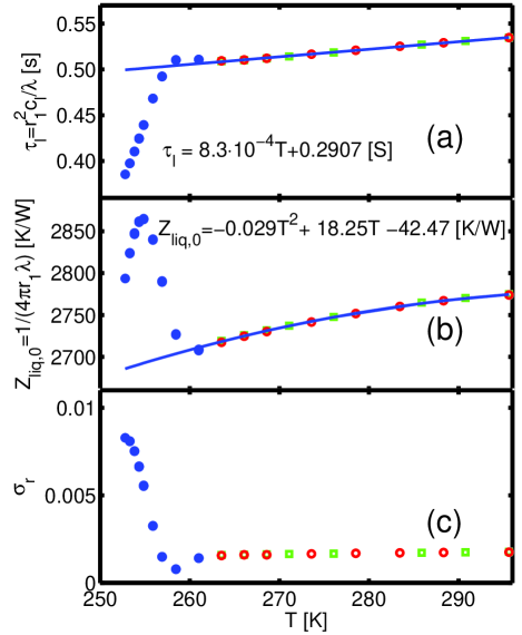
Figure 8: Results from fitting the measured thermal impedance, $Z$, to the $5$-parameter thermal network model (Fig. 6) of the spherical heat effusion experiment Eqs. (9), (42) and (43). This figure shows (a) $\tau_{l}$, (b) $Z_{\text{liq},0}$, and (c) the relative error from the fit, $\sigma_{r}=\sqrt{\frac{\sum_{\nu}|Z-Z_{\text{model}}|^{2}}{\sum_{\nu}|Z_{\text{model}}|^{2}}}$), (the remaining parameteres are shown on figure 7)
Open squares (red): Data taken going down in temperature. Open circles (green): Data taken going up in temperature. Closed circles (blue): Low temperature data including points take going down and up. Line: Interpolated temperature dependencies of $\tau_{l}$, and $Z_{\text{liq},0}$ found based on data from above the liquid glass transition temperature range, used for extrapolating down in the region where the liquid relaxation sets in (the functional form and fitting results are shown).

The solid line in Fig. 4 shows the result of such a fit to $Z$-data at room temperature ($295.6$K). The model captures the features in the frequency dependence of the measured thermal impedance very precisely. Also in Fig. 4 is shown the thermal impedance as it would have been if the properties of the thermistor bead itself had been negligible, i.e. if $Z$ was identical to $Z_{\text{liq}}$ of Eq. (9) We note that especially the high frequency behaviors are different but also the limiting value at low frequency is higher for the measured $Z$ than for $Z_{\text{liq}}$. This is due to the additional thermal resistance in the bead capsule layer.

In table 2 we report the results for $\tau_{b}$ and $\hat{c}$ obtained at room temperature. Four values are given for each quantity, they are taken at the two input amplitudes and from an initial measurement at room temperature and a measurement taken at the end of the temperature scan. The method is seen to give very reproducible results.

Table 2: Heat conductivity and specific heat for the liquid ($\lambda$ and $c_{l}$), as defined in relation to Fig. 10 and 12. Fitting parameters characterizing the bead ($\tau_{b}$ and $\hat{c}$) from the fits to the five-parameter mode. The results are at room temperature ($295.6$K), and taken using two input amplitudes $|U_{1}|$. The two scans are the initial scan and a scan taken after the temperature scan coming back to room temperature. The results indicates the reproducibility of the method.

$|U_{1}|$	$P_{2}$	scan	$\tau_{b}$	$\hat{c}=c_{l}/c_{b}$	$\lambda$	$c_{l}$
$[\mathrm{V}]$	$[\mathrm{m}\mathrm{W}]$		$[s]$		$[\mathrm{W}/(\mathrm{K}\cdot\mathrm{m})]$	$[10^{6}\mathrm{J}/(\mathrm{K}\cdot\mathrm{m}^{3})]$
$4.9$	$0.63$	$1$	$0.0665$	$1.0983$	$0.13759$	$1.7597$
		$2$	$0.0666$	$1.0977$	$0.13761$	$1.7602$
$2.9$	$0.23$	$1$	$0.0663$	$1.0989$	$0.13786$	$1.7627$
		$2$	$0.0668$	$1.0953$	$0.13782$	$1.7623$

The five parameters are extrapolated down to the regime of frequency dependent $c_{l}$, by the functions indicated on the figures. $\hat{r}$ is considered being temperature independent. $\hat{c}$, $\tau$ and $\tau_{b}$ are to a good approximation linear in temperature over the investigated temperature range. $Z_{\text{liq},0}$ is found to be very well fitted by a second degree polynomial.

The extrapolated values of the five parameters can then be used for calculating $Z_{\text{liq}}$ from the measured thermal impedance, $Z$ inverting the relations Eqs. (43) and (42). In Fig. 9 the thermal impedance of the liquid, $Z_{\text{liq}}$, and the raw measured thermal impedance, $Z$, are shown for data taken at room temperature ($=295.6\mathrm{K}$).

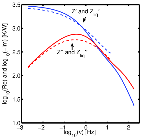
Figure 9: Comparison of the raw measured thermal impedance, $Z$, and final liquid thermal impedance, $Z_{\text{liq}}$, corrected for the influence of the thermistor encapsulation. Data are taken at room temperature ($T=295.6\mathrm{K}$), and are equivalent to the data shown on Fig. 4. The liquid thermal impedance is truncated at high frequencies ($\nu>10^{1.2}\mathrm{Hz}$) as the bead becomes dominant at higher frequencies, leading to unphysical behavior of the calculated liquid impedance. Full lines: Raw thermal impedance $Z$. Dashed lines: Liquid thermal impedance $Z_{\text{liq}}$.

As discussed earlier effusion from a plane plate can only give the effusivity $e=\sqrt{\lambda c}$. Thus the specific heat cannot be found absolutely. In contrast effusion from a sphere is able to give both the heat conductivity and the longitudinal specific heat absolutely even if the latter is frequency dependent. However, the heat conductivity has to be frequency independent to allow for this separation. The separation is possible because $Z_{\text{liq}}$ as given in Eq. (9) has the low frequency limiting value $Z_{\text{liq},0}=1/(4\pi\lambda r_{1})$. The convergence is rather slow involving the squareroot of the frequency. However, if we look at the reciprocal quantity, the thermal admittance $Y_{\text{liq}}=1/Z_{\text{liq}}$

$$Y_{\text{liq}}=4\pi\lambda r_{1}\left(1+\sqrt{i\omega{r_{1}}^{2}c_{l}/\lambda}\right)$$ (45)

we observe that when $c_{l}$ is frequency independent the squareroot frequency term can be cancelled by taking the difference between $Y_{\text{liq}}^{\prime}$ and $Y_{\text{liq}}^{\prime\prime}$

$$\lambda=\frac{Y_{\text{liq}}^{\prime}-Y_{\text{liq}}^{\prime\prime}}{4\pi r_{1}}.$$ (46)

This is valid even in the glass transition range at sufficiently low frequencies where $c_{l}$ reaches its non-complex equilibrium value. Finally, using the found values for $\lambda$ the frequency dependent longitudinal specific heat is calculated from

$$c_{l}(\omega)=\frac{\lambda}{i\omega r_{1}^{2}}\left(\frac{Y_{\text{liq}}}{4\pi\lambda r_{1}}-1\right)^{2}$$ (47)

However the structure of the five parameter model only allows for determining $\hat{r}$ but not $r_{0}$ and $r_{1}$ independently from the fit to data. To obtain the absolute value of $\lambda$ and $c_{l}$ one of the radii are needed. Measured values of $r_{1}$ are given in table 1. As indicated the bead is not completely spherical, and it is therefore needed to determine which value of $r_{1}$ to use.

According to the specifications for Santovac® 5 given by Scientific instrument service, Inc Scientific instrument service, Inc (2008) the value of $\lambda$ at $20\mathrm{\SIUnitSymbolCelsius}$ is $0.1330\mathrm{W}/(\mathrm{K}\cdot\mathrm{m})$. They likewise report the isobaric specific heat pr. mass $c_{p}/\rho=0.35\text{cal}/(\mathrm{g}\cdot\mathrm{K})$ and density $\rho=1.204\mathrm{g}/\mathrm{c}\mathrm{m}^{3}$ at $20\mathrm{\SIUnitSymbolCelsius}$ giving a specific heat pr. volume of $c_{p}=1.76\cdot 10^{6}\mathrm{J}/(\mathrm{K}\cdot\mathrm{m}^{3})$. At these temperatures the isobaric and longitudinal specific heats are identical, we have therefore chosen to use a value for $r_{1}$ which matches $c_{l}$, within the errors, to the reference value. This “optimized” value is very close to the $r_{1,\text{Measured, long edge}}$ value given in table 1. This choice gives a value of $\lambda$ which is $3.5\%$ too big compared to the literature value.

Fig. 10 shows how the temperature dependence of the heat conductivity, $\lambda$, of the sample liquid is found. In Fig. 11 is shown the final frequency dependent specific heat for a number of temperatures. Table 2 reports the room temperature values for $c_{l}$ and $\lambda$ for two temperature amplitudes, and data reproduced after a temperature scan down and up again. The values indicate the reproducibility of the method.

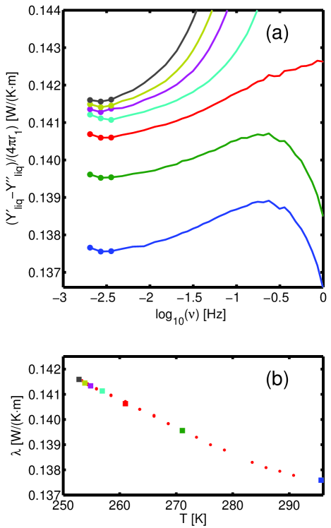
Figure 10: Thermal conductivity of the liquid. (a): $\frac{Y^{\prime}_{\text{liq}}-Y^{\prime\prime}_{\text{liq}}}{4\pi r_{1}}$ as function of frequency, plotted for a selection of temperatures (same temperatures as on Fig. 11, with colors indicating same datasets). According to Eq. 46 the thermal conductivity is the low frequency limit of this quantity. The points on the lines indicate the data points used for defining the low frequency limit (taken as an average over these points). (b): Thermal conductivity of the liquid defined from the average over the low frequency limit of $\frac{Y^{\prime}_{\text{liq}}-Y^{\prime\prime}_{\text{liq}}}{4\pi r_{1}}$. Squares corresponds to the curves shown on the upper figure, and dots to the remaining datasets.

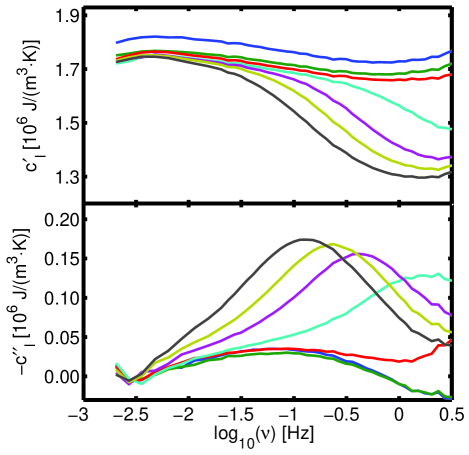
Figure 11: Real and imaginary part of the longitudinal specific heat of the liquid, $c_{l}$, at a number of the investigated temperatures. The frequency axis is truncated at $0.5\mathrm{Hz}$ as the signal above this frequency is dominated by the inner-structure of the thermistor. Temperatures are $295.6\mathrm{K}$, $271.1\mathrm{K}$, $261.0\mathrm{K}$, $256.9\mathrm{K}$, $254.9\mathrm{K}$, $253.8\mathrm{K}$, and $252.8\mathrm{K}$.

VII Discussion

The derived longitudinal specific heat displayed in Fig. 11 shows the expected relaxation phenomena at the glass transition. At $252.7\mathrm{K}$ $c_{l}$ decreases from $c_{0}=c_{l}(\omega\rightarrow 0)=1.75\cdot 10^{6}\mathrm{J}/(\mathrm{K}\cdot{\mathrm{m}}^{3})$ to $c_{\infty}=c_{l}(\omega\rightarrow\infty)=1.30\cdot 10^{6}\mathrm{J}/(\mathrm{K}\cdot{\mathrm{m}}^{3})$. The temperature dependency of $c_{0}$ above the glass transition range is shown in Fig. 12. The temperature dependency of the characteristic relaxation time, $\tau$, is shown in Fig. 13. The high temperature data are seen to show spurious frequency dependency in both the real and imaginary part of $c_{l}$. This may be caused by small systematic errors in the data processing or data acquisition that we have not been able to trace yet. It may also be due to the small eccentricity of the bead. Due to the functional relationship, Eq. (9) between $Z_{\text{liq}}$ and $c_{l}$ a small relative error $|dZ_{\text{liq}}/Z_{\text{liq}}|$ in the thermal impedance may propagate to a large relative error $|dc_{l}/c_{l}|$ in the specific heat. As a function of the dimensionless Laplace-frequency $s=i\omega\tau_{l}$ one finds

$$\frac{dc_{l}}{c_{l}}/\frac{dZ_{\text{liq}}}{Z_{\text{liq}}}=2\frac{1+\sqrt{s}}{\sqrt{s}}.$$ (48)

This factor is four at the characteristic heat diffusion frequency ($s=1$) increasing to a factor of $22$ at $0.01$ times this frequency. Thus the specific heat is difficult to get reliable more than 2 decades below the characteristic diffusion frequency. On the other hand one decade above this frequency the measured $Z$ is dominated by the thermal structure of the thermistor bead that can only to some extent be reliable modelled .

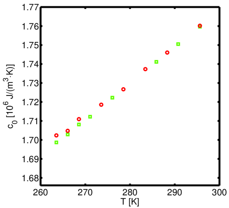
Figure 12: DC specific heat, $c_{0}$, of the liquid for temperatures above the liquid glass transition temperature range. The specific heat is found as the average over the real part of $c_{l}$ in the frequency range $10^{-2}\mathrm{Hz}$–$1\mathrm{Hz}$. $c_{0}$ corresponds to the DC value of $c_{p}$ as can be seen from Eq. (3) and Eq. (4). Open squares (green): Data taken going down in temperature. Open circles (red): Data taken going up in temperature.

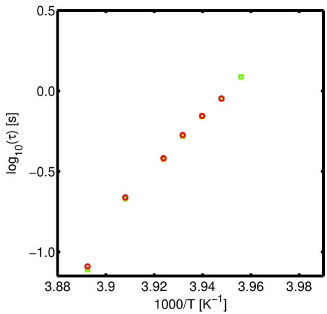
Figure 13: Characteristic relaxation time, $\tau$, for the longitudinal specific heat, $c_{l}(\omega)$. The time if found from a fit to 2.order polynomial to a few point around the maximum of the imaginary part of $c_{l}$ and corresponds to $\tau=1/(2\pi\nu_{\text{lp}})$, where $\nu_{\text{lp}}$ is the frequency of maximum loss. Open squares (green): Data taken going down in temperature. Open circles (red): Data taken going up in temperature.

VIII Conclusion

From a theoretical point of view determination of the frequency dependent specific heat by a thermal effusion method based on a sphere has many ideal features. The surface of a sphere — being closed — has no boundary and thus no associated boundary effects like a finite plane plate. The thermomechanical coupling problem can be treated analytically i.e. the influence of the increasing dynamic shear modulus and the mechanical boundary conditions are adequately taken into account. Although the thermomechanical problem can also be solved in the onedimensional unilateral case it is not so obvious whether it really applies to the experimental finite plate realizations. It is of course preferable if thermal experiments can give two independent thermal properties e.g. the specific heat and the heat conductivity or the effusivity and diffusivity. Effusion experiments in different geometries give the effusivity only unless a characteristic length scale comes into play with the heat diffusion length. For the infinite plane there is no such length scale whereas in the spherical case this length scale is the radius of the heat producing sphere. This advantage is however also the weakness of the method since it limits the practical frequency window to be studied.

Appendix A The AC-method to higher order

In this appendix we analyze which higher-order terms must be included in order to get a relative accuracy of $1\cdot 10^{-4}$ on the measured temperature amplitude from the Fourier components of the measured voltages of the voltage divider (see Fig. 1).

In the following we will include up to fourth harmonics in all the relevant quantities, hence we write

$$V(t) = \frac{1}{2}\left(V_{0}+V_{1}E_{1}+V_{2}E_{2}+V_{3}E_{3}+V_{4}E_{4}+c.c.\right)$$ (49a)

$$U(t) = \frac{1}{2}\left(U_{0}+U_{1}E_{1}+U_{2}E_{2}+U_{3}E_{3}+U_{4}E_{4}+c.c.\right)$$ (49b)

$$P(t) = \frac{1}{2}\left(P_{0}+P_{1}E_{1}+P_{2}E_{2}+P_{3}E_{3}+P_{4}E_{4}+c.c.\right)$$ (49c)

$$\Delta T(t) = \frac{1}{2}\left(T_{0}+T_{1}E_{1}+T_{2}E_{2}+T_{3}E_{3}+T_{4}E_{4}+c.c.\right).$$ (49d)

Combining the expansion of the thermistor resistance to second order, Eq. (34), with the voltage divider equation, Eq. (16), the voltage across the preresistor becomes, to second order in $\Delta T$,

$$V(t)=\frac{1}{A+1}\left(1-a\Delta T+b\Delta T^{2}\right)U$$ (50)

with $A=R_{0}/R_{\text{pre}}$, $a=\frac{A\alpha_{1}}{1+A}$ and $b=\left(\frac{A\alpha_{1}}{1+A}\right)^{2}-\frac{A\alpha_{2}}{1+A}$.

If this expression is explicitly calculated using the above expansions of $U$ and $T$ (Eq. (49b) and (49d)) a large number of terms is obtained. In the following we make a numerical inspection of which terms are most significant, in a worst case, to reduce the number of terms included.

In order to calculate the order of magnitude of the terms, an estimate of the size of the components of $U$ and $\Delta T$ are needed. In Fig. 14 we show the relative magnitudes of the different components of the input voltage, $U$, of the voltage divider to $U_{1}$. In table 3 we summarize the upper limits of these ratios. In Fig. 15 we show the relative magnitude of the different components of the power calculated from the measured $U_{i}$ and $V_{i}$ components. In table 4 we summarize the upper limits on these ratios. We estimate the relative size of the temperature amplitudes as equal to the relative sizes of the power amplitudes. In table 5 we give characteristic values of the quantities describing the thermistor and the resistors.

Combing the estimates given in table 5, with Eq. (26), we observe that a change in $T_{2}$ of $1\cdot 10^{-4}\mathrm{K}$ corresponds to a change in $V_{3}/U_{1}$ of $5\cdot 10^{-7}$. Hence only terms in the expansion of Eq. (50) which are larger than $5\cdot 10^{-7}U_{1}$ will be included.

By explicit substitution of Eq. (49b) and (49d) into Eq. (50) and insertion of the estimates from table 3, 4 and 5 the following expressions are found for the first and third harmonics on the voltage, $V$, when disregarding terms smaller than $5\cdot 10^{-7}U_{1}$

$$V_{1}=\frac{1}{A+1}\left[U_{1}-aT_{0}U_{1}-\frac{1}{2}aT_{2}U_{1}^{*}+X_{1}\right]$$ (51a)

and

$$V_{3}=\frac{1}{A+1}\left[-\frac{1}{2}aT_{2}U_{1}+U_{3}+X_{3}\right]$$ (51b)

with

$$X_{1} = -aT_{1}U_{0}+bT_{0}^{2}U_{1}+\frac{1}{2}bT_{2}T_{2}^{*}U_{1}+bT_{0}T_{2}U_{1}^{*}$$ (51c)

$$X_{3} = -\frac{1}{2}aT_{4}U_{1}^{*}+\frac{1}{4}bT_{2}^{2}U_{1}^{*}+bT_{0}T_{2}U_{1}+bT_{0}T_{4}U_{1}^{*}.$$ (51d)

Appendix B Power terms to higher order

The relevant set of power components are calculated from Eq. (30) as

$$P=\frac{(U-V)V}{R_{\text{pre}}}$$

using the expansions in Eq. (49a) and (49b) to be

$$P_{0} = \frac{1}{R_{\text{pre}}}\left(W_{0}V_{0}+\frac{1}{2}\mathrm{Re}\left(W_{1}V_{1}^{*}+W_{2}V_{2}^{*}+W_{3}V_{3}^{*}+W_{4}V_{4}^{*}\right)\right)$$ (52a)

$$P_{1} = \frac{1}{R_{\text{pre}}}\left(W_{{1}}V_{{0}}+V_{{1}}W_{{0}}+\frac{1}{2}\left(W_{{2}}V_{{1}}^{*}+W_{{1}}^{*}V_{{2}}+W_{{3}}V_{{2}}^{*}+W_{{2}}^{*}V_{{3}}+W_{3}^{*}V_{4}+W_{4}V_{3}^{*}\right)\right)$$ (52b)

$$P_{2} = \frac{1}{R_{\text{pre}}}\left(W_{{0}}V_{{2}}+W_{{2}}V_{{0}}+\frac{1}{2}\left(W_{{1}}V_{{1}}+W_{{1}}^{*}V_{{3}}+W_{2}^{*}V_{4}+W_{{3}}V_{{1}}^{*}+W_{4}V_{2}^{*}\right)\right)$$ (52c)

$$P_{3} = \frac{1}{R_{\text{pre}}}\left(W_{{0}}V_{{3}}+W_{{3}}V_{{0}}+\frac{1}{2}\left(W_{{1}}V_{{2}}+W_{{2}}V_{{1}}+W_{1}^{*}V_{4}+W_{4}V_{1}^{*}\right)\right)$$ (52d)

$$P_{4} = \frac{1}{R_{\text{pre}}}\left(W_{0}V_{4}+W_{4}V_{0}+\frac{1}{2}\left(W_{1}V_{3}+W_{2}V_{2}+W_{3}V_{1}\right)\right)$$ (52e)

where $W=U-V$.

Appendix C The “five parameter” formulation of the thermal transfer model

Eq. (9) , (41) and(42) are in the following written in terms of the five variables

$$\tau_{l}=r_{1}^{2}\frac{c_{l}}{\lambda},\quad\tau_{b}=r_{1}^{2}\frac{c_{b}}{\lambda_{b}},\quad\hat{r}=\frac{r_{0}}{r_{1}},\quad\hat{c}=\frac{c_{l}}{c_{b}},\quad Z_{\text{liq},0}=\frac{1}{4\pi\lambda r_{1}}.$$ (53)

The thermal impedance, Eq. (9), is given as

$$Z_{\text{liq}}=Z_{\text{liq},0}\frac{1}{\left(1+\sqrt{i\omega\tau_{l}}\right)}\,$$ (54)

The components of the thermal transfer matrix Christensen and Dyre (2008) in Eq. (41) are given as

$$T^{\rm th}_{11}\, = \,\hat{r}\cosh\big{(}\sqrt{i\omega\tau_{b}}(1-\hat{r})\big{)}+\frac{1}{\sqrt{i\omega\tau_{b}}}\sinh\big{(}\sqrt{i\omega\tau_{b}}(1-\hat{r})\big{)}$$ (55a)

$$T^{\rm th}_{12}\, = \,-Z_{\text{liq},0}\frac{\hat{c}}{\tau_{l}}\frac{\sqrt{i\omega\tau_{b}}}{\hat{r}}{\sinh\big{(}\sqrt{i\omega\tau_{b}}(1-\hat{r})\big{)}}{}$$ (55b)

$$T^{\rm th}_{21}\, = \,\frac{1}{Z_{\text{liq},0}}\frac{\tau_{l}}{\hat{c}}\frac{1}{\left(\sqrt{i\omega\tau_{b}}\right)^{3}}\Big{[}\big{(}1-i\omega\tau_{b}\hat{r}\big{)}\sinh\big{(}\sqrt{i\omega\tau_{b}}(1-\hat{r})\big{)}-\sqrt{i\omega\tau_{b}}(1-\hat{r})\cosh\big{(}\sqrt{i\omega\tau_{b}}(1-\hat{r})\big{)}\Big{]}$$ (55c)

$$T^{\rm th}_{22}\, = \,\frac{1}{\hat{r}}\cosh\big{(}\sqrt{i\omega\tau_{b}}(1-\hat{r})\big{)}-\frac{1}{\hat{r}\sqrt{i\omega\tau_{b}}}\sinh\big{(}\sqrt{i\omega\tau_{b}}(1-\hat{r})\big{)}$$ (55d)

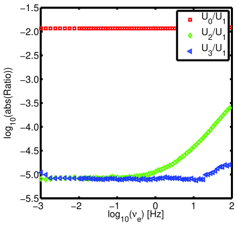
Figure 14: Relative magnitude of the components of input voltage $U$ to the dominant $U_{1}$ component. $\langle|U_{1}|\rangle=4.909\mathrm{V}$. See also table 3.

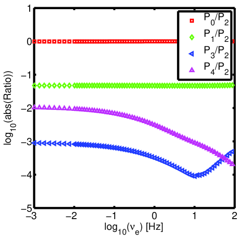
Figure 15: Magnitude of the components of the power to the dominant $P_{2}$ component. $\langle|U_{1}|\rangle=3.927\mathrm{V}$, $T_{\text{cryo}}=249.5\mathrm{K}$. See also table 4.

Table 3: Maximum of relative magnitude of the components of input voltage $U$ to the dominant first harmonic $U_{1}$, as shown on Fig. 14 (for $\nu<40\mathrm{Hz}$).

$U_{0}/U_{1}$	$U_{2}/U_{1}$	$U_{3}/U_{1}$	$U_{4}/U_{1}$
$2\cdot 10^{-2}$	$10^{-4}$	$10^{-5}$	$3\cdot 10^{-5}$

Table 4: Maximum of relative magnitude of the components of the power as shown on Fig. 15, (for $\nu<40\mathrm{Hz}$).

$P_{0}/P_{2}$	$P_{1}/P_{2}$	$P_{3}/P_{2}$	$P_{4}/P_{2}$
$1$	$10^{-1}$	$10^{-3}$	$10^{-2}$

Table 5: Characteristic sizes of the parameters describing the used thermistor at $T_{\text{cryo}}=249.5\mathrm{K}$

$A$	$\alpha_{1}$	$\alpha_{2}$
$\approx 2$	$\approx 4\cdot 10^{-2}\reciprocal\mathrm{K}$	$\approx 10^{-3}\mathrm{K}^{-2}$

References

- Harrison (1976) G. Harrison, The Dynamic Properties of Supercooled Liquids (Academic, New York, 1976).
- Davies and Jones (1953) R. O. Davies and G. O. Jones, Adv. Phys. 2, 370 (1953).
- Birge and Nagel (1985) N. O. Birge and S. R. Nagel, Phys. Rev. Lett. 54, 2674 (1985).
- Christensen (1985) T. Christensen, J. Phys. (Paris) Colloq. 46, 635 (1985).
- Christensen and Olsen (1998) T. Christensen and N. B. Olsen, J. Non-Cryst. Solids 235–237, 296 (1998).
- Huth et al. (2007) H. Huth, A. A. Minakov, A. Serghei, F. Kremer, and C. Schick, Eur. Phys. J. Special Topics 141, 153 (2007).
- Birge (1986) N. O. Birge, Phys. Rev. B 34, 1631 (1986).
- Moon et al. (1996) I. K. Moon, Y. H. Jeong, and S. I. Kwun, Rev. Sci. Instrum. 67, 29 (1996).
- Birge et al. (1997) N. O. Birge, P. K. Dixon, and N. Menon, Thermochim. Acta 304-305, 51 (1997).
- Minakov et al. (2001) A. A. Minakov, S. A. Adamovsky, and C. Schick, Thermochim. Acta 377, 173 (2001).
- Minakov et al. (2003) A. A. Minakov, S. A. Adamovsky, and C. Schick, Thermochim. Acta 403, 89 (2003).
- Christensen et al. (2007) T. Christensen, N. B. Olsen, and J. C. Dyre, Phys. Rev. E 75, 041502 (2007).
- Christensen et al. (2008) T. Christensen, N. B. Olsen, and J. C. Dyre, in 5th International Workshop on Complex Systems, edited by M. Tokuyama, I. Oppenheim, and H. Nishiyama (AIP, Melville, NY, 2008, 2008), vol. 982 of AIP Conf. Proc., p. 139.
- Christensen and Dyre (2008) T. Christensen and J. C. Dyre, Phys. Rev. E 78, 021501 (2008).
- Christensen and Olsen (1994) T. Christensen and N. B. Olsen, Phys. Rev. B 49, 15396 (1994).
- Carslaw and Jaeger (1959) H. S. Carslaw and J. C. Jaeger, Conduction of heat in solids (Clarendon Press, Oxford, 1959).
- Landau and Lifshitz (1986) L. D. Landau and E. M. Lifshitz, Theory of Elasticity (Pergamon, London, 1986), 3rd ed.
- Birge and Nagel (1987) N. O. Birge and S. R. Nagel, Rev. Sci. Instrum. 58, 1464 (1987).
- Igarashi et al. (2008a) B. Igarashi, T. Christensen, E. H. Larsen, N. B. Olsen, I. H. Pedersen, T. Rasmussen, and J. C. Dyre, Rev. Sci. Instrum. 79, 045105 (2008a).
- Igarashi et al. (2008b) B. Igarashi, T. Christensen, E. H. Larsen, N. B. Olsen, I. H. Pedersen, T. Rasmussen, and J. C. Dyre, Rev. Sci. Instrum. 79, 045106 (2008b).
- Scientific instrument service, Inc (2008) Scientific instrument service, Inc, Specifications for santovac 5 and santovac 5p ultra, Web page (2008), URL http://www.sisweb.com/catalog/08/F14.