SISSA-63/2008/EP

Which BPS Baryons Minimize Volume?

Jarah Evslin

Scuola Internazionale Superiore di Studi Avanzati (SISSA),
Strada Costiera, Via Beirut n.2-4, 34013 Trieste, Italia

Stanislav Kuperstein

Theoretische Natuurkunde, Vrije Universiteit Brussel and
The International Solvay Institutes
Pleinlaan 2, B-1050 Brussels, Belgium

Abstract

A BPS 3-cycle in a Sasaki-Einstein 5-manifold in general does not minimize volume in its homology class, as we illustrate with several examples of non-minimal volume BPS cycles on the 5-manifolds $Y^{p,q}$. Instead they minimize the energy of a wrapping D-brane, extremizing a generalized calibration. We present this generalized calibration and demonstrate that it reproduces both the Born-Infeld and the Wess-Zumino parts of the D3-brane energy.

1 Introduction

A D-brane wrapping a BPS cycle minimizes the energy in its (twisted) homology class [1, 2]. In the absence of fluxes, the energy is equal to the volume of the wrapped cycle and so BPS D-branes wrap minimal volume cycles [1]. In the presence of fluxes, the energy is equal to the sum of a Born-Infeld contribution, which contains the volume, and Wess-Zumino contributions, which consist of various fluxes. Therefore in general energy and volume are not minimized by the same cycles [2, 3].

In this note we will understand this observation from the viewpoint of generalized calibrations. In particular we will present a generalized calibration that calibrates 3-cycles on all Sasaki-Einstein 5-manifolds. While generalized calibrations have been studied extensively in the context of generalized Calabi-Yau 6-manifolds, to our knowledge, the only Sasaki-Einstein manifold on which a generalized calibration has been presented so far is the 5-sphere [4]. We will report then a number of explicit examples of non-BPS 3-cycles with lower volumes than BPS 3-cycles in the same homology class on Sasaki-Einstein manifolds $Y^{p,q}$ (see [5]).

A generalized calibration on a manifold $M$ endowed with a closed $(p+2)$-form $F_{p+2}$ is a $p$-form $\phi_{p}$ such that when pulled back to any $p$-dimensional subbundle $E$ of the tangent bundle $TM$:

$$i:E\hookrightarrow TM,\hskip 19.91684pti^{*}\phi_{p}\leqslant\textrm{d}\textrm{Vol}_{E},$$ (1.1)

where $\textrm{d}\textrm{Vol}_{E}$ is the volume form on the subbundle, and such that there exists some unit Killing vector $\xi$ satisfying:

$$\textrm{d}\phi_{p}=i_{\xi}F_{p+2}.$$ (1.2)

If we compactify type II string theory on a $(p+2)$-dimensional manifold $M^{p+2}$, with $F_{p+2}$ the RR $(p+2)$-form field strength, then the Noether energy density of a D$p$-brane with respect to the light-like Killing vector $\xi$ is the sum of the Born-Infeld contribution $\textrm{Vol}_{E}$ and the Wess-Zumino contribution $i_{\xi}C_{p+1}$, where $C_{p+1}$ is the potential for $F_{p+2}$ in some gauge. The brane has minimal energy in its homology class when the inequality in (1.1) is saturated [2, 3]. In this case the cycle $\Sigma^{p}$ wrapped by the D$p$-brane is said to be calibrated by $\phi_{p}$. In particular, the D$p$-brane can only be BPS with respect to the Killing spinor $\epsilon$ if the cycle is calibrated with respect to the Killing vector:

$$\xi_{\mu}=\overline{\epsilon}\Gamma_{\mu}\epsilon,$$ (1.3)

where $\Gamma_{\mu}$’s are gamma matrices.

In Section 2 we will introduce a generalized calibration for Sasaki-Einstein 5-folds with a specific RR flux. In Section 3 we will explicitly calculate the volumes of some BPS 3-cycles in $Y^{p,q}$ and we will find that sometimes non-BPS cycles in the same homology class have smaller volumes than BPS cycles. In Section 4 we specialize the argument of [2] that D3-branes wrapping BPS 3-cycles of unequal volumes nonetheless have the same energy to the case of generalized calibrations on Sasaki-Einstein 5-manifolds. This argument is then applied to BPS 3-cycles in $Y^{p,q}$. Finally in the conclusion we provide a formula for the energies of branes wrapping non-BPS cycles. The generalized calibration implies that these are necessarily greater than those of branes wrapping BPS cycles in the same homology class, but we provide an explicit example in which this is indeed the case, even though BPS cycles have a larger volume.

2 The generalized calibration

2.1 The proposal

To define a generalized calibration one needs to choose the vector $\xi$ in (1.2). The manifold $M^{5}$ is Euclidean, and so there are no available light or time-like vectors, instead we will choose the Reeb vector. Therefore $\xi$ will not satisfy (1.3). Nevertheless the generalized calibration constructed from $\xi$ will summarize the BPS condition, because $\xi$ is the spatial part of a light-like Killing vector whose temporal part does not contribute to the energy of D-branes wrapping nontrivial cycles in $M^{5}$ (see Section 4 for a related discussion).

More precisely, consider the geometry $AdS_{5}\times M^{5}$ where $C(M^{5})$ is the Calabi-Yau cone over the $5d$ Sasaki-Einstein space $M^{5}$. The preserved $10d$ Killing spinor $\widetilde{\epsilon}$ may be decomposed into the tensor product of a Killing spinor $\chi$ on $AdS_{5}$ and a Killing spinor $\epsilon$ on $M^{5}$:

$$\widetilde{\epsilon}=\chi\otimes\epsilon.$$ (2.1)

One may use this Killing spinor to define a one-form:

$$\widetilde{\eta}=(\overline{\widetilde{\epsilon}}\Gamma_{\mu}\widetilde{\epsilon})\,\textrm{d}x^{\mu}.$$ (2.2)

The temporal part of $\widetilde{\eta}$ comes entirely from the temporal part of the geometry, in the $AdS_{5}$ factor. It will contribute to (1.2), however $i_{\partial/\partial t}F_{5}$ pulled back to cycles on the Sasaki-Einstein will vanish and so we will not be interested in this contribution. Instead, we will be interested only in the contribution $\eta$ of the Sasaki-Einstein part of the Killing spinor:

$$\eta=(\overline{\epsilon}\Gamma_{\mu}\epsilon)\textrm{d}x^{\mu},$$ (2.3)

which is the contact form of $M^{5}$ [6]. The contact form is dual to the Reeb vector $\xi$. Therefore a D3-brane on $M^{5}$ will be BPS if and only if it saturates the bound (1.1) where $\phi_{3}$ satisfies (1.2) with $\xi$ equal to the unit Reeb vector.

The metric on $M^{5}$ may be decomposed as:

$$\textrm{d}s^{2}_{M^{5}}=\textrm{d}s^{2}_{KE}+\eta\otimes\eta,$$ (2.4)

where $ds^{2}_{KE}$ is Kähler-Einstein metric on the subspace of the tangent bundle of $M^{5}$ which is orthogonal to the Reeb vector field. When $M^{5}$ is regular, as in the case $M^{5}=T^{1,1}$, then $M^{5}$ is just a circle fibration over a Kähler Einstein base and $\eta$ is the vertical form plus connection. In this section we will not restrict our analysis to the $Y^{p,q}$ [5] or the $L^{a,b,c}$ [7] family of spaces, considering instead a general non-singular 5-dimensional Sasaki-Einstein manifold.

The metric of the Calabi-Yau cone $C(M^{5})$ over $M^{5}$ is simply:

$$\textrm{d}s^{2}_{C(M^{5})}=\textrm{d}r^{2}+r^{2}\textrm{d}s^{2}_{M^{5}},$$ (2.5)

where $r$ is the radial direction on the cone, $M^{5}$ is embedded at $r=1$. If $J_{KE}$ is the Kähler form of the 4-dimensional Kähler-Einstein metric, then the Kähler form $J$ of the Calabi-Yau is:

$$J=\frac{1}{2}\textrm{d}\left(r^{2}\eta\right)=r^{2}J_{KE}+r\textrm{d}r\wedge\eta,$$ (2.6)

where we used the fact that $\textrm{d}\eta=2J_{KE}$. The Calabi-Yau is calibrated by an ordinary (closed) calibration:

$$\frac{1}{2}J\wedge J=r^{3}\textrm{d}r\wedge J_{KE}\wedge\eta+\frac{1}{2}r^{4}J_{KE}\wedge J_{KE}=r^{3}\textrm{d}r\wedge\alpha_{3}+r^{4}\beta_{4},$$ (2.7)

where we have defined:

$$\alpha_{3}=J_{KE}\wedge\eta\qquad\textrm{and}\qquad\beta_{4}=\frac{1}{2}J_{KE}\wedge J_{KE}.$$ (2.8)

The 4-dimensional calibrated cycles $C(\Sigma^{3}_{k})$ of $C(M^{5})$ are cones over the 3-cycles $\Sigma^{3}_{k}$ of $M^{5}$. This means that the pullbacks of the calibration $\frac{1}{2}J\wedge J$ to the cycles $C(\Sigma^{3}_{k})$ are equal to their volume forms:

$$I_{k}:C(\Sigma^{3}_{k})\hookrightarrow C(M^{5}),\hskip 19.91684ptI_{k}^{*}\left(\frac{1}{2}J\wedge J\right)=\textrm{d}\textrm{Vol}_{C(\Sigma^{3}_{k})}=r^{3}\textrm{d}r\wedge\textrm{d}\textrm{Vol}_{\Sigma^{3}_{k}},$$ (2.9)

where $\textrm{d}\textrm{Vol}_{C(\Sigma^{3}_{k})}$ and $\textrm{d}\textrm{Vol}_{\Sigma^{3}_{k}}$ are the volume forms on $C(\Sigma^{3}_{k})$ and $\Sigma^{3}_{k}$ respectively, and we have used the conic structure of the $6d$ metric to find the relation between the two volume forms. Pushing forward via the projection map:

$$\pi:C(M^{5})\longrightarrow M^{5},$$ (2.10)

which integrates away the $\textrm{d}r$ factors, we arrive at:

$$i_{k}:\Sigma^{3}_{k}\hookrightarrow M^{5},\hskip 19.91684pti_{k}^{*}(\alpha_{3})=\textrm{d}\textrm{Vol}_{\Sigma^{3}_{k}},$$ (2.11)

where the embedding $i_{k}$ is the restriction of the embedding $I_{k}$ in (2.9) to $\Sigma^{3}_{k}$. Therefore $\alpha_{3}$ pulled back to $M^{5}$, which we also denote $\alpha_{3}$, is a 3-form such that, when pulled back to the base $\Sigma^{3}_{k}$ of a BPS cycle $C(\Sigma^{3}_{k})$, it is equal to the volume form. This motivates the following proposal [8]:

The 3-form $\alpha_{3}=J_{KE}\wedge\eta$ is a generalized calibration for Sasaki-Einstein 5-folds with respect to the Reeb vector $\xi$, when $F_{5}$ from (1.2) is equal to four times the volume form.

Notice that in type IIB supergravity compactifications on $AdS_{5}\times M^{5}$, the RR flux 5-form is indeed four times the volume form of the Sasaki-Einstein space $M^{5}$. For concreteness we have restricted our attention to Sasaki-Einstein 5-folds, but $\alpha_{2k+1}=\frac{1}{k!}J_{KE}^{k}\wedge\eta$ is a generalized calibration for any Sasaki-Einstein $(2k+3)$-manifold.

2.2 The demonstration

To check this proposal, one must verify that the inequality (1.1) holds for all 3-cycles $\Sigma^{3}$ in $M^{5}$ and also that (1.2) is satisfied. Let $\Sigma^{3}$ be a 3-cycle in $M^{5}$ such that (1.1) is not satisfied. In other words:

$$i:\Sigma^{3}\hookrightarrow M^{5},\hskip 19.91684pti^{*}\alpha_{3}>\textrm{d}\textrm{Vol}_{\Sigma^{3}},$$ (2.12)

where $\textrm{d}\textrm{Vol}_{\Sigma^{3}}$ is the volume form of $\Sigma^{3}$.

Let $C(\Sigma^{3})$ be the cone over $\Sigma^{3}$, which has volume form $r^{3}\textrm{d}r\wedge\textrm{d}\textrm{Vol}_{\Sigma^{3}}$. Multiplying (2.12) by $r^{3}\textrm{d}r$ one finds that the volume form of $C(\Sigma^{3})$ is less then the integral of the pullback of a particular four-form $\gamma_{4}\equiv r^{3}\textrm{d}r\wedge\alpha_{3}$:

$$I:C(\Sigma^{3})\hookrightarrow C(M^{5}),\hskip 19.91684ptI^{*}\gamma_{4}=I^{*}\left(r^{3}\textrm{d}r\wedge\alpha_{3}\right)>r^{3}\textrm{d}r\wedge\textrm{d}\textrm{Vol}_{\Sigma^{3}}=\textrm{d}\textrm{Vol}_{C(\Sigma^{3})}.$$ (2.13)

As the cone $C(\Sigma^{3})$ is the product of the radial direction and an orthogonal 3-fold, the pullback to $C(\Sigma^{3})$ of a 4-form with all legs along the base is zero. In particular, the pullback of $\beta_{4}$ to $C(\Sigma^{3})$ is zero, and so the pullback of the calibrating 4-form $\frac{1}{2}J\wedge J$ is equal to that of $r^{3}\textrm{d}r\wedge\alpha_{3}$. In summary:

$$I^{*}\left(\frac{1}{2}J\wedge J\right)=I^{*}(r^{3}\textrm{d}r\wedge\alpha_{3})>\textrm{d}\textrm{Vol}_{C(\Sigma^{3})}.$$ (2.14)

This is in contradiction with the fact that $\frac{1}{2}J\wedge J$ is a calibration on $C(M^{5})$, therefore no such 3-cycle $\Sigma^{3}$ may exist and so $\alpha_{3}$ satisfies the inequality (1.1) with respect to all 3-cycles.

Now we need to show that $\alpha_{3}$ also satisfies the condition (1.2). Indeed, since $\textrm{d}\eta=2J_{KE}$ we find that:

$$\textrm{d}\alpha_{3}=2J_{KE}\wedge J_{KE}.$$ (2.15)

On the other hand, the volume 6-form of $C(M^{5})$ is $\textrm{d}\textrm{Vol}_{C(M^{5})}=\frac{1}{6}J\wedge J\wedge J$ and thus the volume 5-form on $M^{5}$ is $\textrm{d}\textrm{Vol}_{M^{5}}=\frac{1}{2}J_{KE}\wedge J_{KE}\wedge\eta$. Since the contact form $\eta$ and the Reeb vector $\xi$ are dual, namely $i_{\xi}\eta=1$, we finally obtain that:

$$\textrm{d}\alpha_{3}=4\cdot i_{\xi}\textrm{d}\textrm{Vol}_{M^{5}}=i_{\xi}F_{5}$$ (2.16)

in accordance with the condition (1.2). Therefore $\alpha_{3}$ is indeed a generalized calibration for $M^{5}$ with $F_{5}=4\cdot\textrm{d}\textrm{Vol}_{M^{5}}$.

3 Calculating volumes of submanifolds

Consider a cone $C(Y^{p,q})$ over a Sasaki-Einstein base $Y^{p,q}$. The cone is Calabi-Yau and so it is calibrated by the 4-form $\frac{1}{2}J\wedge J$, where $J$ is its Kähler form. The cone $C(Y^{p,q})$ is the Kähler quotient of $\mathbb{C}^{4}\backslash\{\mathbb{C}^{2}\cup\mathbb{C}^{2}\}$ by a $\mathbb{C}^{*}$ action under which the complex coordinates $(z_{1},z_{2},z_{3},z_{4})$ transform with weights $(-p,-p,p-q,p+q)$. The 4-dimensional submanifolds on which $z_{i}$ vanish are divisors $C(\Sigma_{i}^{3})$ of $C(Y^{p,q})$. They are interesting because they are calibrated. Their volumes are infinite, however their volume density is equal to the pullback of $\frac{1}{2}J\wedge J$ to their world-volumes [5].

At large $N$, we are not interested precisely in the divisors $C(\Sigma_{i}^{3})$ , but rather in their 3-dimensional bases $\Sigma_{i}^{3}$. Branes that wrap these bases are also BPS. The near-horizon geometry of a stack of $N$ D3-branes at the tip of the conifold $C(T^{1,1})$ is $AdS_{5}\times T^{1,1}$ with $N$ units of RR 5-form flux on the $T^{1,1}$. Based on the ideas of [9] it was conjectured in [10] (see also [11]) that the BPS (di-)baryons in the dual CFT [12] are dual to D3-branes wrapped on the 3-cycles $\Sigma_{i}^{3}$ on the $T^{1,1}$ which are the bases of the divisors $z_{i}=0$. The conjecture relies on the fact that $T^{1,1}$ has the topology of $S^{3}\times S^{2}$ and in particular [12, 13, 14]:

$$\hbox{\rm H}_{3}\left(T^{1,1}\right)=\mathbb{Z}$$ (3.1)

and so the homology class of a 3-cycle is a single integer. Remarkably, $Y^{p,q}$ (and $L^{a,b,c}$) has the same $S^{3}\times S^{2}$ topology and so the conjecture of [10] has been naturally extended to the CFT models based on the $AdS_{5}\times Y^{p,q}$ geometries [5]. The homology classes of the bases of the divisors are just equal to the weights of the $\mathbb{C}^{*}$ quotient, in other words it is $(-p)$ for the base $\Sigma_{1,2}^{3}$ of the $z_{1,2}=0$ cycles and $(p-q)$ and $(p+q)$ for the $z_{3}=0$ and $z_{4}=0$ cycles $\Sigma_{3}^{3}$ and $\Sigma_{4}^{3}$ respectively.

The goal of this section is to find the minimal volumes of three-spheres representing the third homology class $1\in\mathbb{Z}$ in $Y^{p,q}$ spaces for $q=1$ and arbitrary $p$. We begin with a partial review of the results of [15], where the $Y^{p,q}$ spaces were trivialized for arbitrary $p$ and $q=1$ or $2$, restricting our attention to the $q=1$ case.

First we must properly normalize the Kähler quotient coordinates $z_{i}$ discussed in the previous section. For $q=1$ the D-term condition on the reduction reads:

$$p\left(|z_{1}|^{2}+|z_{2}|^{2}\right)-(p-1)|z_{3}|^{2}-(p+1)|z_{4}|^{2}=0.$$ (3.2)

We are interested only in the $5d$ $Y^{p,1}$ base of the $6d$ $C(Y^{p,1})$ cone. Away from the tip (where all $z_{i}$’s vanish) we can introduce new variables:

$$\left(u_{1},u_{2},v_{1},v_{2}\right)=\Lambda^{-p}\left(z_{1},z_{2},\sqrt{1-\frac{1}{p}}\bar{z}_{3},\sqrt{1+\frac{1}{p}}\bar{z}_{4}\right).$$ (3.3)

The normalization factor $\Lambda$ is fixed by the requirement that both vectors, $u$ and $v$, have unit length. Unlike the conifold case here $\Lambda$ depends not only on the radial coordinate $r$ appearing in the conic metric (2.5) but also on one of the coordinates of the $Y^{p,q}$ base (see below).

Next we notice that under the $U(1)$ gauge transformation of the Kähler quotient $u$ and $v$ transform like

$$\left(u_{1},u_{2}\right)\to e^{i\lambda p}\left(u_{1},u_{2}\right)\qquad\textrm{and}\qquad\left(v_{1},v_{2}\right)\to\left(e^{i\lambda(p-1)}v_{1},e^{i\lambda(p+1)}v_{2}\right),$$ (3.4)

so the vector $w=(w_{1},w_{2})$ defined by:

$$\left(\begin{array}[]{c}w_{1}\\ w_{2}\end{array}\right)=\left(\begin{array}[]{cc}u_{1}&-u_{2}^{\star}\\ u_{2}&u_{1}^{\star}\end{array}\right)\left(\begin{array}[]{c}v_{1}^{\star}\\ -v_{2}\end{array}\right)$$ (3.5)

transforms like $w\to e^{i\lambda}w$. It also has unit length. By means of the Hopf fibration $w$ describes an $S^{2}$. To parameterize the remaining $S^{3}$ we need:

$$\widehat{w}=c_{\widehat{w}}\left(w_{1}^{p},w_{2}^{p}\right)\qquad\textrm{where}\qquad c_{\widehat{w}}=1/\sqrt{|w_{1}|^{2p}+|w_{2}|^{2p}},$$ (3.6)

so the length-one $\widehat{w}$ transforms exactly like $u$:

$$\widehat{w}\to e^{i\lambda p}\widehat{w}.$$ (3.7)

With $u$ and $\widehat{w}$ in hand we define a special unitary matrix $X\in SU(2)$:

$$X=u\widehat{w}^{\dagger}-\epsilon u^{\star}\widehat{w}^{\textrm{{T}}}\epsilon,$$ (3.8)

which is $U(1)$-invariant and thus properly defines an $S^{3}$. To summarize, starting from a $Y^{p,1}$ given by $u$ and $v$, we may find the $w$ and then $X$ that describe the $S^{2}$ and the $S^{3}$ respectively. Alternatively beginning with $X$ and $w$ we can determine $\widehat{w}$ from $w$ and then $u$ from the identity:

$$u=X\widehat{w},$$ (3.9)

that follows directly from the definition of $X$. Finally, (3.5) can be used to find $v$.

To calculate the volumes of the 3-cycles we must identify the spheres in terms of the metric coordinates. The $5d$ $Y^{p,q}$ metric is:

$$\textrm{d}s^{2}_{Y^{p,q}} = \frac{1-y}{6}\left(\textrm{d}\theta^{2}+\sin^{2}\theta\textrm{d}\phi^{2}\right)+\frac{\textrm{d}y^{2}}{H(y)}+\frac{H(y)}{36}\left(\textrm{d}\beta+\cos\theta\textrm{d}\phi\right)^{2}+$$ (3.10)

$$+\frac{1}{9}\left(\textrm{d}{\psi^{\prime}}-\cos\theta\textrm{d}\phi+y\left(\textrm{d}\beta+\cos\theta\textrm{d}\phi\right)\right)^{2},$$

where

$$H(y)=\left(2\frac{a-3y^{2}+2y^{3}}{1-y}\right)^{1/2}.$$ (3.11)

In these coordinates one can immediately identify the Reeb vector $\xi$ and the contact form $\eta$ in (3.10):

$$\eta=\frac{1}{3}\left(\textrm{d}{\psi^{\prime}}-\cos\theta\textrm{d}\phi+y\left(\textrm{d}\beta+\cos\theta\textrm{d}\phi\right)\right),\qquad\xi=3\frac{\partial}{\partial\psi^{\prime}}$$ (3.12)

and the 2-forms $J$ and $J_{KE}$ can be easily derived using the formulae of the previous section.

The coordinates $\phi$ and $\psi^{\prime}$ are $2\pi$-periodic, while the azimuthal coordinates $\theta$ and $y$ inhabit the ranges $\theta\in[0,\pi]$ and $y\in[y_{1},y_{2}]$, where the constants $y_{1}$ and $y_{2}$ are the smallest two roots of the numerator in (3.11) and are determined by:

$$y_{1,2}=\frac{1}{4p}\left(2p\mp 3q-\sqrt{4p^{2}-3q^{2}}\right).$$ (3.13)

These relations also fix the constant $a$ in (3.11). The third $2\pi$-periodic angular coordinate is:

$$\tau=\frac{p+q}{2}(\phi+\psi^{\prime})-\frac{1}{6\ell}(\beta+\psi^{\prime})\qquad\textrm{where}\qquad\ell\equiv\frac{q}{3q^{2}-2p^{2}+p\sqrt{4p^{2}-3q^{2}}}.$$ (3.14)

In [15] the gauge invariant variables built from the Kähler quotient $\mathbf{C}^{4}$ coordinates $z_{i}$ were matched with the independent non-singular holomorphic functions on $C(Y^{p,q})$. The comparison yielded an explicit dependence of the $z_{i}$’s on the metric coordinates. This dependence, of course, included a free complex parameter. The absolute value of this parameter is the normalization parameter $\Lambda$ used in (3.3) and the phase $\lambda$ corresponds to the $U(1)$ gauge of the Kähler quotient mentioned in (3.4).

With the connection between $z_{i}$’s and the azimuthal coordinates $\theta$ and $y$ we can identify the $z_{i}=0$ divisors in terms of the metric coordinates. It appears that the bases of the divisors $z_{1}=0$ and $z_{2}=0$ correspond to $\theta=0$ and $\theta=\pi$ respectively. Similarly $z_{3}=0$ and $z_{4}=0$ are related to $y=y_{1}$ and $y=y_{2}$. On the other hand, our three-sphere (defined in [15] by $w_{2}=0$) is given by the embedding $\psi^{\prime}=\textrm{const}$ and $\theta=\theta(y)$, where the latter is a very complicated function that can be found only numerically. The explicit form of the function, however, is not significant if we only want to compute the flux of the RR $3$-form through the 3-sphere. To this end it is sufficient to know only the boundary conditions which are [15]:

$$\theta(y_{1})=\pi\qquad\textrm{and}\qquad\theta(y_{2})=0.$$ (3.15)

The $3$-form is also a generator of the third cohomology class, so the computation provides a decisive check of our $S^{3}$ identification. The RR $3$-form $F_{3}$ is a real part of the self-dual $(2,1)$ form $G_{3}$ found in [16] (see also [17]). The RR $2$-form potential is given by:

$$C_{2}=\frac{p^{2}-q^{2}}{16\pi^{2}}\left(\frac{1}{1-y}\textrm{d}\psi^{\prime}\wedge\textrm{d}\beta+\frac{\cos\theta}{1-y}\textrm{d}\psi^{\prime}\wedge\textrm{d}\phi+\frac{y\cos\theta}{1-y}\textrm{d}\beta\wedge\textrm{d}\phi\right),$$ (3.16)

where $\beta$ is related to the $2\pi$-periodic $\tau$ by (3.14). Substituting $q=1$, $\textrm{d}\psi^{\prime}=0$ and $\theta=\theta(y)$ into $\textrm{d}C_{2}$ one can easily verify that the flux is one as expected for a representative of the homology class $1\in\mathbb{Z}$.

Again, here only the boundary values (3.15) of $\theta(y)$ play an important rôle. This is because $C_{2}$ is globally well-defined except on the submanifolds $y=(y_{1},y_{2})$ and $\theta=(0,\pi)$, where the Dirac strings are located (see [15]).

Our strategy, therefore, will be as follows. Since for the initial values (3.15) of the function $\theta=\theta(y)$ and with $\psi^{\prime}=\textrm{const}$ the homology class of the $3$-cycle is always one, we may find a function $\theta_{\textrm{min}}=\theta(y)$, which satisfies (3.15) and at the same time minimizes the volume of the $3$-sphere. Although we have not found a proof that this ansatz indeed leads to the minimal possible volume of the homology class one cycle, this approach is certainly sufficient for our needs, since our main goal is to show that the volume of the non-BPS cycle is smaller than that of a BPS cycle representing the same homology class. The situation is summarized in Figure 1.

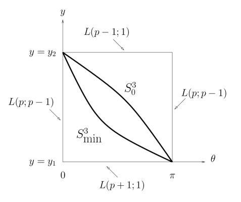
Figure 1: This picture shows various $3$-cycles of $Y^{p,1}$ on the $(\theta,y)$ plane. Only the lines on the boundary represent supersymmetric cycles. For $y=y_{1,2}$ and $\theta=0,\pi$ one finds three different lens spaces (see footnote 2) with the homology classes $(-p)$, $(p-1)$ and $(p+1)$. One solid curve is the non-BPS three-sphere $S_{0}^{3}$ found in [15] and the other shows the non-BPS $3$-sphere profile $S^{3}_{\textrm{min}}$ that generally minimizes the volume.Note that both curves start and end at the same points. Also on both curves the $2\pi$-periodic angles along the $3$-sphere are $\phi$ and $\tau$, while $\psi^{\prime}$ is kept constant.

Finding the profile $\theta(y)_{\textrm{{min}}}$, which provides the minimum volume $3$-sphere, amounts to solving a complicated $2nd$ order differential equation (ODE) with the initial conditions (3.15). This equation is provided in the Appendix. We solved it numerically for $p=2,3,4$ and $5$. We then used this numerical solution to compute the volumes. Since we are obliged to exploit a numerical approach both for the solution of the ODE and for the integration of the volume, the final result will be inevitably a bit imprecise.

In order to reach a decisive conclusion regarding the volume comparison, we will also compute volumes for the following test profile:

$$\cos(\theta_{\textrm{Test}}(y))=\frac{2y-y_{2}-y_{1}}{y_{2}-y_{1}}.$$ (3.18)

The volume calculation for $\theta_{\textrm{Test}}$ turns out to be very accurate. We will see that even for this probe function the final volumes are usually smaller than their BPS counterparts, though this is not a solution of the ODE. In what follows we report our results for the aforementioned values of $p$. As in the previous section we will denote the $3d$ bases of the $4d$ $z_{i}=0$ divisors by $\Sigma_{i}$. These BPS $3$-cycles are lens spaces and represent homology classes $-p$, $-p$, $p-1$ and $p+1$ for $\Sigma_{1}^{(-p)}$, $\Sigma_{2}^{(-p)}$, $\Sigma_{3}^{(p-1)}$ and $\Sigma_{4}^{(p+1)}$ respectively, where for the sake of clarity we have added superscripts indicating their homology classes. The volumes of the cycles are:

$$\textrm{Vol}\left(\Sigma_{1,2}^{(-p)}\right) = \frac{4\pi^{2}}{3}\ell$$

$$\textrm{Vol}\left(\Sigma_{3}^{(p-1)}\right) = -\frac{8\pi^{2}}{3}\ell y_{1}(1-y_{1})$$

$$\textrm{Vol}\left(\Sigma_{4}^{(p+1)}\right) = \frac{8\pi^{2}}{3}\ell y_{2}(1-y_{2}).$$ (3.19)

Notice that for any $p$ the BPS cycles $\Sigma_{1,2}^{(-p)}\bigcup\Sigma_{3}^{(p-1)}$ and $\Sigma_{1,2}^{(-p)}\bigcup\Sigma_{4}^{(p+1)}$ have homology classes $\pm 1$. For our purposes we will have to compare the cycle with the smallest volume among the two with the non-BPS homology class one cycles we have described above. Finally, the cycles corresponding to $\theta_{\textrm{Test}}(y)$ and $\theta_{\textrm{min}}(y)$ will be denoted by $\Sigma_{\textrm{Test}}$ and $\Sigma_{\textrm{min}}$.

3.1 $Y^{3,1}$

For $p=3$ we found:

$$\frac{\textrm{Vol}\left(\Sigma_{\textrm{Test}}\right)}{4\pi^{2}}\approx 0.133358(0)\qquad\textrm{and}\qquad\frac{\textrm{Vol}\left(\Sigma_{\textrm{min}}\right)}{4\pi^{2}}\approx 0.129(8).$$ (3.20)

On the other hand:

$$\frac{\textrm{Vol}\left(\Sigma_{1,2}^{(-3)}\right)}{4\pi^{2}} = \frac{5+\sqrt{33}}{144}\approx 0.074615(0)$$

$$\frac{\textrm{Vol}\left(\Sigma_{3}^{(2)}\right)}{4\pi^{2}} = \frac{19+4\sqrt{33}}{432}\approx 0.083874(3)$$

$$\frac{\textrm{Vol}\left(\Sigma_{4}^{(4)}\right)}{4\pi^{2}} = \frac{7+\sqrt{33}}{216}\approx 0.059002(6).$$ (3.21)

We see that although the BPS cycles $\Sigma_{i}$ have very small volumes compared to $\Sigma_{\textrm{Test}}$ and $\Sigma_{\textrm{min}}$, still the minimal volume of a BPS homology class one cycle is bigger than $\textrm{Vol}\left(\Sigma_{\textrm{Test}}\right)$:

$$\frac{\textrm{Vol}\left(\Sigma_{1}^{(-3)}\bigcup\Sigma_{4}^{(4)}\right)}{4\pi^{2}}\approx 0.133617(6)>\frac{\textrm{Vol}\left(\Sigma_{\textrm{Test}}\right)}{4\pi^{2}}>\frac{\textrm{Vol}\left(\Sigma_{\textrm{min}}\right)}{4\pi^{2}}.$$ (3.22)

As was advertised in the previous section we find that the $3$-sphere with a minimal volume in the homology class $1\in\mathbb{Z}$ is non-BPS.

3.2 $Y^{4,1}$

For $p=4$ the volumes are:

$$\frac{\textrm{Vol}\left(\Sigma_{\textrm{Test}}\right)}{4\pi^{2}}\approx 0.100597(5)\qquad\textrm{and}\qquad\frac{\textrm{Vol}\left(\Sigma_{\textrm{min}}\right)}{4\pi^{2}}\approx 0.099(1)$$ (3.23)

and:

$$\frac{\textrm{Vol}\left(\Sigma_{1,2}^{(-4)}\right)}{4\pi^{2}} = \frac{29+4\sqrt{61}}{1080}\approx 0.055778(7)$$

$$\frac{\textrm{Vol}\left(\Sigma_{3}^{(3)}\right)}{4\pi^{2}} = \frac{43+5\sqrt{61}}{1728}\approx 0.047483(3)$$

$$\frac{\textrm{Vol}\left(\Sigma_{4}^{(5)}\right)}{4\pi^{2}} = \frac{91+11\sqrt{61}}{2880}\approx 0.061428(0).$$ (3.24)

Thus for the homology class one cycles we have:

$$\frac{\textrm{Vol}\left(\Sigma_{1}^{(-4)}\bigcup\Sigma_{3}^{(3)}\right)}{4\pi^{2}}\approx 0.103262(1)>\frac{\textrm{Vol}\left(\Sigma_{\textrm{Test}}\right)}{4\pi^{2}}>\frac{\textrm{Vol}\left(\Sigma_{\textrm{min}}\right)}{4\pi^{2}}.$$ (3.25)

So, again, we can draw very firm conclusions.

3.3 $Y^{5,1}$

For $p=5$ the volumes are:

$$\frac{\textrm{Vol}\left(\Sigma_{\textrm{Test}}\right)}{4\pi^{2}}\approx 0.080690(4)\qquad\textrm{and}\qquad\frac{\textrm{Vol}\left(\Sigma_{\textrm{min}}\right)}{4\pi^{2}}\approx 0.080(0)$$ (3.26)

and

$$\frac{\textrm{Vol}\left(\Sigma_{1,2}^{(-5)}\right)}{4\pi^{2}} = \frac{47+5\sqrt{97}}{2160}\approx 0.044557(5)$$

$$\frac{\textrm{Vol}\left(\Sigma_{3}^{(4)}\right)}{4\pi^{2}} = \frac{133+13\sqrt{97}}{5400}\approx 0.048339(8)$$

$$\frac{\textrm{Vol}\left(\Sigma_{4}^{(6)}\right)}{4\pi^{2}} = \frac{73+7\sqrt{97}}{3600}\approx 0.039428(3)$$ (3.27)

Thus for the homology class one cycles we have:

$$\frac{\textrm{Vol}\left(\Sigma_{1}^{(-5)}\bigcup\Sigma_{4}^{(6)}\right)}{4\pi^{2}}\approx 0.083985(9)>\frac{\textrm{Vol}\left(\Sigma_{\textrm{Test}}\right)}{4\pi^{2}}>\frac{\textrm{Vol}\left(\Sigma_{\textrm{min}}\right)}{4\pi^{2}}.$$ (3.28)

This time the BPS cycle has $5\%$ bigger volume the non-BPS cycle and the results suggest that the ratio grows as one increases $p$.

3.4 $Y^{2,1}$

The $p=2$ case is very special, since the cycle $\Sigma_{3}^{(1)}$ is both BPS and homology class one. Its volume is:

$$\frac{\textrm{Vol}\left(\Sigma_{3}^{(1)}\right)}{4\pi^{2}}=\frac{31+7\sqrt{13}}{432}\approx 0.130182(5).$$ (3.29)

We also found that:

$$\frac{\textrm{Vol}\left(\Sigma_{\textrm{min}}\right)}{4\pi^{2}}\approx 0.185(0).$$ (3.30)

Although we were not able to calculate $\textrm{Vol}\left(\Sigma_{\textrm{min}}\right)$ with higher accuracy, the answer is significantly bigger than $\textrm{Vol}\left(\Sigma_{3}^{(1)}\right)$ and so for $Y^{2,1}$ the minimum volume $3$-sphere is apparently BPS. It is natural to propose that a BPS cycle will minimize the volume in the homology class $1$ for all of the $Y^{p,p-1}$ spaces, including $Y^{1,0}=T^{1,1}$, since in these cases $\Sigma_{3}^{(1)}$ is both BPS and also a homology class $1\in\mathbb{Z}$ cycle. This is a natural proposal, as in these cases the divisor $C(\Sigma^{(}1)_{3})$, which is a cone over a representative of the element $1$ in the third homology group, is an irreducible variety.

4 Energies of BPS Cycles

BPS states are necessarily either stable or marginally stable. In particular, no state with the same conserved charges may have a lower energy. In the present context, this implies for example that D3-branes wrapping generalized calibrated cycles in a Sasaki-Einstein 5-fold cannot decay. If there were two such cycles representing the same homology class, then a transition between them would be allowed and so such branes must have the same energy. We have already seen examples of generalized calibrated 3-cycles in the same homology class with different volumes, therefore the Born-Infeld contribution to their energies, which measures their volumes, must be precisely compensated by the Wess-Zumino contribution to their energy. Such a cancellation is guaranteed by the general arguments of [2]. In this section we will apply these general arguments to the specific case of generalized calibrated 3-cycles on a Sasaki-Einstein 5-fold. As the RR gauge potential $C_{4}$ extends along 4 Sasaki-Einstein directions, and the BPS D3-branes only extend along 3, one may have concluded that the Wess-Zumino terms play no role. We will now see that this is not the case.

For simplicity, we will consider a D3-brane with a vanishing gauge potential wrapped on the 3-cycle $\Sigma^{3}$. Then the DBI action just produces its volume. If the cycle is calibrated by a calibration $\alpha_{3}=J_{KE}\wedge\eta$, then the volume is just equal to the integral of $\alpha_{3}$. Now we want to show that the total energy of this D-brane is the same as that of any other D-brane wrapped on any other calibrated 3-cycle $\widetilde{\Sigma^{3}}$ in the same homology class as $\Sigma^{3}$. Formally this is equivalent to showing that the energy of a brane on $\Sigma^{3}$ plus an anti-brane (with no absolute value in the DBI energy) on $\widetilde{\Sigma^{3}}$ is equal to zero, which is in turn equivalent to showing that the energy of a brane on a calibrated cycle of trivial homology is equal to zero. It is this last statement that we will show. So we may assume that $\Sigma^{3}$ is homologically trivial, and so there exists some 4-chain $B^{4}$ whose boundary is $\Sigma^{3}$.

How does one calculate the energy associated with the DBI and Wess-Zumino terms in the action? First of all, energy is the charge corresponding to some translational symmetry. Therefore one must choose a direction in which to perform the translation. The BPS condition imposes that the energies with respect to a vector $\xi$ given by the preserved SUSYs (1.3) is the same for all BPS cycles. Therefore we will be interested in the energy with respect to this vector. We claim that if all of the fields and connections have a zero Lie derivative with respect to $\xi$, then the energy density with respect to $\xi$ is just the interior product $i_{\xi}$ of the Lagrangian density. To calculate the total energy, one pulls back the energy density to a surface at a constant time and then integrates.

This prescription is perhaps more familiar in electrostatics. The Lagrangian of a particle of charge one contains the 1-form potential $A_{\mu}$. The energy of the particle is just the interior product of $A_{\mu}$ with the time vector ${\partial_{t}}$, which is:

$$i_{\partial_{t}}A=A_{0}$$ (4.1)

often called the scalar potential. The scalar potential is only well defined up to an additive constant, which cancels when one considers the difference between the energies of two particles. We are interested in the difference in the energies between two branes, and so this additive constant will cancel. Notice that gauge transformations can change $A_{0}$ by more than just a constant, but when the magnetic field is time-independent one may always choose a gauge in which $\dot{A_{i}}=0$ and so $A_{0}$ is the energy of the electron.

In our case the field strength $F_{5}$ is time-independent and so the Wess-Zumino energy is just $C_{4}$ contracted with our temporal vector. On the other hand the DBI energy is just the 4-volume contracted with the temporal vector. The $\xi$ part of the temporal vector contracted with the 4-volume form on the D3-brane worldvolume gives a form with one leg along time, which vanishes when pulled back to a spatial slice, therefore only the $i_{\partial_{t}}(\textrm{d}t\wedge\textrm{d}\textrm{Vol}_{\Sigma^{3}})$ contributes to the DBI energy, which for a generalized calibrated cycle is just the calibration form $\alpha_{3}$. Summarizing, the Wess-Zumino energy density is $i_{\xi}C_{4}$ and the DBI energy density is the spatial volume form.

In a supersymmetric configuration, the metric and the field strengths are invariant under a translation along the Reeb vector field $\xi$. Therefore there exists a gauge such that the RR gauge potential $C_{4}$ is also invariant:

$$\mathcal{L}_{\xi}C_{4}=\textrm{d}i_{\xi}C_{4}+i_{\xi}F_{5}=0.$$ (4.2)

In this gauge the Wess-Zumino contribution to the energy density of our brane is just $i_{\xi}C_{4}$. Technically, one needs to use the sum of the Reeb vector of the Sasaki-Einstein manifold with that of the $AdS_{5}$, but the latter will not contribute to the energy for a D3-brane which is only 1-dimensional in the AdS directions, like ours. The Wess-Zumino energy can then be calculated using (4.2) and Stokes’ theorem:

$$\mathcal{E}_{\rm{WZ}}=\int_{\Sigma^{3}}i_{\xi}C_{4}=\int_{B^{4}}\textrm{d}i_{\xi}C_{4}=-\int_{B^{4}}i_{\xi}F_{5}=-\int_{B^{4}}\textrm{d}\alpha_{3}=-\int_{\Sigma^{3}}\alpha_{3},$$ (4.3)

where in the fourth equality we used the property (1.2) of generalized calibrations. We have just argued that the integral of $\alpha_{3}$ is the DBI energy, and so we have shown that the Wess-Zumino energy over a trivial calibrated cycle is precisely minus the Wess-Zumino energy, and so the total energy is equal to zero. Therefore the energies of branes on homologous generalized calibrated cycles are equal. In other words, homologous BPS D-branes have the same energy.

The above argument is well-known. In the Sasaki-Einstein case we have considered in this paper, we may be a bit more explicit. We saw in Section 2 that the RR field strength is:

$$F_{5}=2J_{KE}\wedge J_{KE}\wedge\eta$$ (4.4)

and so its interior product with respect to the Reeb vector is just:

$$i_{\xi}F_{5}=2J_{KE}\wedge J_{KE}=\textrm{d}\alpha_{3}.$$ (4.5)

The explicit expression for $\xi$ and $\eta$ in the $Y^{p,q}$ case appear in (3.12) and for any Sasaki-Einstein 5-manifold $\textrm{d}\eta=2J_{KE}$. It is also not too difficult to find the 4-chain $B^{4}$ for $Y^{p,q}$’s. Let us consider 3-cycles $\Sigma_{1}^{(-p)}$ and $\Sigma_{3}^{(p-q)}$ introduced in Section 3. Obviously, $\Sigma^{3}=(p-q)\Sigma_{1}^{(-p)}+p\Sigma_{3}^{(p-q)}$ is a trivial 3-cycle. The cone $C(B^{4})$ over the 4-chain $\partial B^{4}=\Sigma^{3}$ is then given by $\hbox{\rm Arg}(z_{1}^{p-q}z_{3}^{p})=0$, where $z_{i}$’s are the Kähler quotient coordinates of Section 3. In particular, recall that $\Sigma_{i}$ is a 3-dimensional base of the cone $z_{i}=0$. The variables $z_{1}$ and $z_{3}$ have quotient charges $-p$ and $p-q$ respectively and so this product is gauge invariant. In the dual gauge theory it corresponds to a mesonic operator.

5 Prospects: Energies of Non-BPS Cycles

The energy of a non-BPS cycle is greater than that of a BPS cycle in the same homology class. The difference is the failure of the bound (1.1) to be saturated. In other words, the difference in energies between a BPS and a non-BPS cycle in the same homology class, including both DBI and Wess-Zumino contributions, is:

$$\Delta\mathcal{E}=\textrm{Vol}_{\Sigma}-\int_{\Sigma}\alpha_{3},$$ (5.1)

where, again, $\Sigma$ is the cycle wrapped by the D3-brane. The generalized calibration condition (1.1) guarantees that this difference is never negative, and so BPS cycles minimize energy. For example, in the case of $Y^{3,1}$ a brane wrapping the cycle $\Sigma_{\textrm{min}}$ will have an energy which is greater than that of a BPS cycle in the same homology class ($1\in\mathbb{Z}=\hbox{\rm H}_{3}(Y^{3,1})$) by:

$$\frac{\Delta\mathcal{E}}{4\pi^{2}}\approx 0.056(7)$$ (5.2)

despite the fact that all such BPS cycles have greater volumes. In other words, the flux causes a D3-brane wrapped on $\Sigma_{\textrm{min}}$ to expand.

It would be interesting to interpret the values of the energies of these operators in the dual gauge theory. Gubser and Klebanov [10] have argued that, in the case of BPS operators on $T^{1,1}$, the volume of the cycle corresponds to the conformal weight. This conjecture has subsequently been extended to BPS cycles in other Sasaki-Einstein’s. If one may find the 3-cycle dual to a given non-chiral operator with a baryonic charge, even in $T^{1,1}$, then (5.1) may be used to compute the energy of that operator and thus to try to determine the corresponding gauge theory quantity.

Appendix

Here we report the differential equation that we had to solve in order to find the three-sphere with the minimal volume. To derive this equation one has to substitute the $\theta=\theta(y)$, $\textrm{d}\psi=0$ ansatz into (3.10) and to calculate the $3$-cycle volume from the induced metric. The variation with respect to $\theta(y)$ then gives the following equation:

$$\left(\left(\frac{w(y)\left(\frac{1-y}{6}\sin(\theta)^{2}+\frac{v(y)}{9}\cos(\theta)^{2}\right)}{\frac{1-y}{6}{\theta^{\prime}_{y}}^{2}+\frac{1}{w(y)v(y)}}\right)^{1/2}\frac{1-y}{6}\theta^{\prime}_{y}\right)^{\prime}_{y}=$$ (5.3)

$$\quad\quad=\left(\frac{w(y)\left(\frac{1-y}{6}{\theta^{\prime}_{y}}^{2}+\frac{1}{w(y)v(y)}\right)}{\frac{1-y}{6}\sin(\theta)^{2}+\frac{v(y)}{9}\cos(\theta)^{2}}\right)^{1/2}\left(\frac{1-y}{6}-\frac{v(y)}{9}\right)\sin(\theta)\cos(\theta),$$

where

$$w(y)=\frac{2(a-y^{2})}{1-y}\qquad\textrm{and}\qquad v(y)=\frac{a-3y^{2}+2y^{3}}{a-y^{2}}.$$ (5.4)

References

- [1] R. Harvey and H. B. Lawson Jr., Calibrated geometries, Acta Math. 148, 47, (1982)
- [2] J. Gutowski and G. Papadopoulos, AdS calibrations, [arXiv:hep-th/9902034] J. Gutowski, G. Papadopoulos and P. K. Townsend, Supersymmetry and generalized calibrations, [arXiv:hep-th/9905156] J. Gutowski, Generalized calibrations, [arXiv:hep-th/9909096] P. K. Townsend, PhreMology: Calibrating M-branes, [arXiv:hep-th/9911154]
- [3] L. Martucci and P. Smyth, Supersymmetric D-branes and calibrations on general N = 1 backgrounds, [arXiv:hep-th/0507099] J. Evslin and L. Martucci, D-brane networks in flux vacua, generalized cycles and calibrations, [arXiv:hep-th/0703129] D. Martelli and J. Sparks, G-Structures, Fluxes and Calibrations in M-Theory, [arXiv:hep-th/0306225]
- [4] E. J. Hackett-Jones and D. J. Smith, Type IIB Killing spinors and calibrations, [arXiv:hep-th/0405098]
- [5] J. P. Gauntlett, D. Martelli, J. Sparks and D. Waldram, Sasaki-Einstein metrics on , [arXiv:hep-th/0403002] D. Martelli and J. Sparks, Toric geometry, Sasaki-Einstein manifolds and a new infinite class of AdS/CFT duals, [arXiv:hep-th/0411238] M. Bertolini, F. Bigazzi and A. L. Cotrone, New checks and subtleties for ads/cft and a-maximization, [arXiv:hep-th/0411249] S. Benvenuti, S. Franco, A. Hanany, D. Martelli and J. Sparks, An infinite family of superconformal quiver gauge theories with Sasaki-Einstein duals, [arXiv:hep-th/0411264]
- [6] D. Martelli, J. Sparks and S. T. Yau, Sasaki-Einstein manifolds and volume minimisation, [arXiv:hep-th/0603021] C. Bär, Real Killng spinors and Holonomy, Commun. Math. Phys. 154 (1993) 509-521
- [7] M. Cvetic, H. Lu, D. N. Page and C. N. Pope, New Einstein-Sasaki spaces in five and higher dimensions, [arXiv:hep-th/0504225] D. Martelli and J. Sparks, Toric Sasaki-Einstein metrics on , [arXiv:hep-th/0505027] S. Benvenuti and M. Kruczenski, From Sasaki-Einstein spaces to quivers via BPS geodesics: , [arXiv:hep-th/0505206] S. Franco, A. Hanany, D. Martelli, J. Sparks, D. Vegh and B. Wecht, Gauge theories from toric geometry and brane tilings, [arXiv:hep-th/0505211] A. Butti, D. Forcella and A. Zaffaroni, The dual superconformal theory for manifolds, [arXiv:hep-th/0505220] M. Cvetic, H. Lu, D. N. Page and C. N. Pope, New Einstein-Sasaki and Einstein spaces from Kerr-de Sitter, [arXiv:hep-th/0505223] S. Kuperstein, O. Mintkevich and J. Sonnenschein, On the pp-wave limit and the BMN structure of new Sasaki-Einstein spaces, [arXiv:hep-th/0609194]
- [8] J. Sparks, private communication.
- [9] E. Witten, Baryons and branes in anti-de Sitter space, [arXiv:hep-th/9805112]
- [10] S. S. Gubser and I. R. Klebanov, Baryon spectra and AdS/CFT correspondence, [hep-th/9808075]
- [11] D. Berenstein, C. P. Herzog and I. R. Klebanov, Baryon spectra and AdS/CFT correspondence, [hep-th/0202150] C. E. Beasley, BPS branes from baryons, [hep-th/0207125]
- [12] I. R. Klebanov and E. Witten, Superconformal Field Theory on Threebranes at a Calabi-Yau Singularity, [arXiv:hep-th/9807080]
- [13] P. Candelas and X. C. de la Ossa, Comments on Conifolds, Nucl. Phys. B 342, 246-268 (1990).
- [14] J. Evslin and S. Kuperstein, Trivializing and orbifolding the conifold’s base, [arXiv:hep-th/0702041]
- [15] J. Evslin and S. Kuperstein, Trivializing a Family of Sasaki-Einstein Spaces, [arXiv:0803.3241]
- [16] C. P. Herzog, Q. J. Ejaz and I. R. Klebanov, Cascading RG flows from new Sasaki-Einstein manifolds, [arXiv:hep-th/0412193]
- [17] J. Evslin, C. Krishnan and S. Kuperstein, Cascading quivers from decaying D-branes, [arXiv:0704.3484]