A Generic Top-Down Dynamic-Programming Approach to Prefix-Free Coding

Abstract

Given a probability distribution over a set of $n$ words to be transmitted, the Huffman Coding problem is to find a minimal-cost prefix free code for transmitting those words. The basic Huffman coding problem can be solved in $O(n\log n)$ time but variations are more difficult. One of the standard techniques for solving these variations utilizes a top-down dynamic programming approach.

In this paper we show that this approach is amenable to dynamic programming speedup techniques, permitting a speedup of an order of magnitude for many algorithms in the literature for such variations as mixed radix, reserved length and one-ended coding. These speedups are immediate implications of a general structural property that permits batching together the calculation of many DP entries.

1 Introduction

Optimal prefix-free coding, or Huffman coding, is a standard compression technique. Consider an encoding alphabet $\Sigma=\{\sigma_{1},\ldots,\sigma_{r}\}$. A code $W=\{w_{1},w_{2},\ldots,w_{n}\}$ is a set of code words $w_{i}\in\Sigma^{*}$. Code $W$ is prefix-free if $\forall w,w^{\prime}\in W$ $w$ is not a prefix of $w^{\prime}.$ As an example, $\{01,00,100\}$ is a prefix-free code but $\{01,00,001\}$ is not, because $00$ is a prefix of $001$.

For $w\in\Sigma^{*}$, let $|w|$ devote the length of $w,$ i.e., the number of characters in $w.$ For example $|0101|=4.$

The input to the problem is a discrete probability distribution $P=\{p_{1},p_{2},\ldots,p_{n}\}$, $\sum_{i}p_{i}=1,$ $\forall i,\,p_{i}\geq 0.$

The output is a a prefix-free code $W=\{w_{1},w_{2},\ldots,w_{n}\}$ whose expected encoding length $\sum_{i=1}^{n}p_{i}|w_{i}|$ is minimized over all $n$ word prefix-free codes. Formally set $Cost(W,P)=\sum_{i=1}^{n}w_{i}p_{i}$. Then

$$Cost(P)=\min_{\mathrel{{}\mathop{\mbox{\footnotesize$W$ is prefix-free}}\limits^{W^{\prime}\subseteq\Sigma^{*},\,|W^{\prime}|=n}}}Cost(W^{\prime},P)$$ (1)

In [16], Huffman gave a classical $O(n\log n)$ time greedy algorithm for solving the binary case ($r=2$) of this problem. Huffman also extended the algorithm to solve the general $r$-ary case with the same time bound. If the $p_{i}$’s are given in sorted order, Huffman’s algorithm can be improved to $O(rn)$ time [20].

The correctness of the Huffman algorithm, although easy to prove, is very strongly dependent upon properties of optimal prefix-free codes. Almost any extra constraint or generalization added to the problem description will invalidate the algorithm’s correctness. Many such constraints/generalizations appear in the literature ([1] is a nice survey) and all require special purpose algorithms to address them.

Some examples of such prefix-free coding problems are Length-limited coding e.g, [17, 18, 3, 19], Unequal-cost coding e.g., [7, 15, 8, 13] Mixed-radix coding [11], Reserved-length coding [4], and One-ended coding [6, 9, 10],

The major observation is that all of the best algorithms known for these problems use some form of dynamic programming (DP) to build an optimal (min-cost) coding tree that corresponds to an optimal code.

These DPs primarily differ in whether they build the tree from the bottom-up or the top-down. The best algorithms for Length-limited and Unequal-cost coding use what essentially reduces to a bottom-up DP model combined with some DP-speedup techniques, e.g., Monge speedups using the SMAWK algorithm of [2] (see [8] for an example of this technique and [19] for a more sophisticated but more specialized speedup method); the best algorithms for Reserved-length and One-ended coding use a top-down DP approach. (Mixed-radix coding [11] uses a totally different DP approach described later)

Length-Limited and Unequal-Cost coding could be solved using a top-down approach but the bottom-up solutions are better for two reasons. The first is that the bottom-up solutions use a more compact solution space than corresponding top-down ones would. This is due to the exploitation of some very problem-specific combinatorial structures of their corresponding optimal code trees. The second is that their bottom-up DPs turn out to have special properties, e.g., the Monge property, which enable speeding up the calculation of table entries. The top-down DPs used in the last two problems don’t have such a compact representations and they also, before this paper, didn’t seem to possess any special property that would lead to speedups.

The main result of this paper is a revisiting of the generic top-down DP approach for solving prefix-free coding problems. We will show that, in this setup, many natural coding problems will have an obvious and simple batching speedup. That is, we will be able to partition the DP table entries into smaller batches (groups) and exploit relationships between entries within a batch to fill in all of the entries in each batch in $O(1)$ amortized time per entry. This will enable speeding up known solutions to the last three problems by at least one factor of $n$. The interesting observation is that the same speedup technique works for all of these problems. Table 1 lists the speedups.

Problem	Previous Best Result	This paper
Mixed Radix Coding	$O(n^{4}\log n)$ [11]	$O(n^{3})$
Reserved Length Coding:
$g$ specific lengths given	$O(gn^{3})$ [4]	$O(gn^{2})$
Reserved Length Coding:
at most $g$ lengths allowed	$O(g^{3}n^{3}\log^{g}n)$ [4]	$O(gn^{2}\log n)$
One-ended Coding	$O(n^{3})$ [10]	$O(n^{2})$

Table 1: A comparison of our new results with previous ones

1.1 The problems

We start by quickly recalling the standard correspondence between prefix-free codes and trees. Let $r=|\Sigma|$ be the size of the alphabet and consider an $r$-ary tree $T$ in which the $i^{\mbox{\footnotesize th}}$edge leaving a node is labelled with character $\sigma_{i}$. Associate with node $v\in T$ the unique word read off walking down the path from the root to $v.$ The set of words $W$ associated with the leaves of $T$ is prefix-free. Conversly, given a prefix-free code $W$ one can build a tree whose leaves are exactly the nodes associated with the words of $W$. See Figure 1

Figure 1: Examples of the code-tree correspondence. Codes are written below their corresponding tree. The leftmost figure is a standard binary tree. The middle is a Mixed-radix tree with level arities $(t_{0},t_{1},t_{2})=(4,2,3).$ The rightmost is a Reserved-length tree with codewords only on levels $\Lambda=\{1,3,5\}$. Note that leaves in all the trees are labelled from top-to bottom

Given tree $T$ associated with code $W$, denote its leaves by $v_{1},v_{2},\ldots,v_{n}$ where $v_{i}$ is the leaf associated with word $w_{i}.$ Let $d(v_{i})$ be the depth of $v_{i}$ in $T.$ By the correspondence, $d(v_{i})=|w_{i}|$ so

$$Cost(T,P)=\sum_{i}d(v_{i})p_{i}=\sum_{i}|w_{i}|p_{i}=Cost(W,P)$$

where $Cost(T,P)$ can be understood as the weighted external-path-length of $T.$ So the prefix-free coding problem is equivalent to finding a tree with minimal external path length. For this reason, most algorithms for finding prefix-free codes are stated as tree algorithms.

We now quickly discuss the problems mentioned in the previous sections and their tree equivalents and then state our new results for these problems.

Mixed-Radix Coding:
In Mixed-Radix Coding the size of the encoding alphabet used depends upon the position of the character within the codeword. This corresponds to constructing a tree in which the arity (number of children) of an internal node depends upon the level of the node. That is, as part of the problem definition, we are given a sequence $t_{0},t_{1},\ldots$ of integers, $t_{i}\geq 2$ such that the maximum arity of a node on level $i$ is $t_{i}.$

The coding version of the problem was motivated [11] by coding with side-channel information and the tree version by problems in multi-level data storage. Chu and Gill [11] solved this problem by introducing an alphabetic version of it and then solving a special case of the alphabetic version. Their algorithm runs in $O(n^{4}\log n)$ time; we will improve this to $O(n^{3})$.

Reserved-Length Coding:
Recall that $|w_{i}|$ is the length of the $i^{\mbox{\footnotesize th}}$codeword. In reserved-length coding there are specific restrictions as to the permitted values of $|w_{i}|$. There are two versions of this problem. In the first version, the given-lengths case, $\Lambda=\{\gamma_{1},\gamma_{2},\ldots,\gamma_{g}\}$ is given as part of the input and we must find a minimum-cost code such that $\forall i,|w_{i}|\in\Lambda$. This corresponds to building a min-cost tree in which all leaves are on levels in $\Lambda.$

In the second version, the $g$-lengths case, $\Lambda$ is not given in advance. The restriction now is to find a minimum-cost code under the restriction that $|\Lambda|\leq g$, where $\Lambda$ is the set of codeword lengths used. This corresponds to building a tree in which at most $g$ levels may contain leaves.

Baer [4] introduces these problems in the context of fast decoding and used a top-down DP approach to solve the first one in $O(|\Lambda|n^{3})$ time and the second one in $O(n^{3}g^{3}\log^{g}n)$ time . We will reduce these two cases, respectively, to $O(|\Lambda|n^{2})$ and $O(n^{2}g\log n)$ time.

One-Ended Coding:
In One-Ended coding the aim is to find a min-cost binary prefix-free code in which every word must end with a 1. This corresponds to finding a min-cost tree in which only right leaves (leaves that are the right children of their parents) are labelled with the $p_{i}$ and counted in the calculation of the cost.

One-Ended Coding was introduced by Berger and Yeung [6] in the context of self-synchronizing codes. Their algorithm ran in exponential time. This was later improved by De Santis, Capocelli and Persiano [9] to another exponential-time algorithm with a smaller exponential base. Chan and Golin [10] showed how to use top-down DP to derive an $O(n^{3})$ time algorithm. We will reduce this down to an $O(n^{2})$ time one.

In Section 2 we introduce a new coding problem called Generalized Mixed-Radix Coding, develop a top-down DP approach for solving it and then speed it up by batching. In Section 3 we reduce both Mixed-Radix Coding and Reduced Length Coding to (multiple) applications of GMR and thus take adavantage of the DP speedup. In Section 4 we reduce the running time of One-Ended coding using an almost identical technique. Since the analysis of One-Ended coding is very similar to that of the GMR problem, we do not provide the details in this extended abstract (but they are available in the appendix).

2 The Top Down DP for Generalized Mixed-Radix Coding

We start by introducing the Generalized Mixed-Radix (GMR) problem, develop a top-down DP for solving it and then see how to speed it up.

In a generalized mixed radix tree, both the arity of an internal node $v$ and the length of an edge leaving $v$ depends on the level of $v$. Figure 2 illustrates these and other definitions in this section. More formally,

Definition 1

Given a a sequence of arities $R=(r_{1},r_{2},\ldots)$ and a sequence of edge length $C=(c_{1},c_{2}\ldots)$, a generalized mixed radix (GMR) tree $T$ satisfying $R$, $C$ is a tree in which internal node $v$ at level $i-1$ has at most $r_{i}$ children and and the length of an edge from $v$ to any of its children is $c_{i}$.

Figure 2: A generalized mixed radix tree with $R=(2,2,2,3,3,4)$ and $C=(1,1,2,2,1,1)$. Note that $n=12$ but to make the tree full we needed to add two extra leavs on the bottom level. Also, the signatures and costs on level $i$ are of the truncated tree containing the nodes on the first $i$ levels. Costs are for $P=\{1,2,3,4,5,6,7,8,9,10,11,12\}$.

We now distinguish between the level $\ell(v)$ of a node v, which is the number of edges from the root to $v$, and its depth, which is the weighted path length from the root to $v$. More formally,

Definition 2

The level of node $v$ in tree $T$ is the number of edges on the unique path from the root to $v$ and will be denoted by $\ell(v).$ The level of tree $T$ is

$$\ell(T)=\max\{\ell(v)\,\mid\,\mbox{$v$ is a node in $T$}\}=\max\{\ell(v)\,\mid\,\mbox{$v$ is a leaf in $T$}\}.$$

The depth of a node on level $i$ of the tree will be the sum of the lengths of the edges on the path from the root to level $i$, i.e., $depth(v)=L(i)=\sum_{j=1}^{i}c_{i}.$ The depth of tree $T$ will be $depth(T)=L(\ell(T)).$

There is an obvious definition of cost in such trees.

Definition 3

Given $R,C$ as above

Let $T$ be any generalized mixed radix tree $T$ for $R,C$ with $n$ leaves labeled $v_{1},v_{2},\cdots,v_{n}$. Then

$$Cost(T)=\sum_{i}depth(v_{i})\cdot p_{i}$$ (2)

The problem to be solved is, given $P$ and $R,C$, find a min-cost tree $T^{*}$ with $n$ leaves, i.e., $Cost(T^{*})=min\left\{Cost(T)\mid\textit{T has $n$ leaves}\right\}$

2.1 The Basic Top-Down Dynamic Program

In this section we quickly describe the standard top-down DP formulation. Since variations of this formulation have been extensively used before for various coding problems, e.g. [15, 12, 10, 4], we only sketch the method but do not rigorously prove its correctness.

In what follows $P=\{p_{1},p_{2},\cdots,p_{n}\}$ with $p_{1}\geq p_{2}\geq\cdots\geq p_{n}\geq 0$ is given and fixed. The $p_{i}$ can be arbitrary weights and are not required to sum to $1$. The $p_{i}$ sequence is implicitly padded so that, for $i>n,$ $p_{i}=0.$ Finally, for $m\geq 0$, set $W_{m}=\sum_{i>m}p_{i}.$

We start with some standard simplifying assumptions about min-cost (optimal) trees $T^{*}$. We will show that there always exists at least one optimal tree satisfying these assumptions. Since our goal is to find any optimal tree, our search can be restricted to trees satisfying the assumptions.

In what follows, an internal node $v$, $\ell(v)=i$, in tree $T$ will be full if and only if it has $r_{i+1}$ children in $T.$ Tree $T$ will be full if all of its internal nodes are full.

Assumption 1: If $i<j$ then, in $T^{*}$, $depth(v_{i})\leq depth(v_{j})$.
If this was not true we could label $v_{i}$ with $p_{j}$ and $v_{j}$ with $p_{i}$. The resulting tree has cost no greater than the original one so it remains optimal. We may therefore always implictly assume that leaf weights in trees are non-increasing in the level of the tree.

Assumption 2: There is a full tree $T^{*}$ with the same cost as the optimal tree for $n$ leaves. $T^{*}$ has $n^{\prime}$ leaves where

$$\max(n,r_{\ell(T^{*})})\leq n^{\prime}\leq n+r_{\ell(T^{*})}-1$$

This will be a consequence of the padding of $P.$

Let $T$ be an optimal tree with exactly $n$ leaves. Suppose $\ell(T)=\ell(v_{n})=\ell$.

First note that all internal nodes $v$ with $\ell(v)<\ell-1$ are full. Otherwise we could add a new leaf child of $v$ at level $\ell(v)+1<\ell(v_{n})$ and label it with $p_{n}$, creating a tree with smaller cost than optimal tree $T.$ Thus, the only non-full internal nodes in $T$ are on level $\ell-1.$

Next note that we may assume that at most one internal node at level $(\ell-1)$ is not full; otherwise leaves on level $i$ can be shifted to the left, so that all internal nodes on level-$(i-1)$, except possibly the rightmost one, are full. Make this rightmost node full by adding an appropriate number leaves to it and call this new full tree $T^{*}$. Note that $\ell(T^{*})=\ell(T)=\ell$ and $cost(T)=cost(T^{*}).$ This follows because $P$ was padded by setting $p_{i}=0$ for $i>n.$ Let $n^{\prime}$ be the number of leaves in $T^{*}$.

By definition $n\leq n^{\prime}.$ Since $T$ contains at least one internal node on level $\ell-1$, $T^{*}$ contains at least $r_{\ell}$ leaves on level $\ell-1.$ Thus $\max(n,r_{\ell})\leq n^{\prime}$

Furthermore, $n^{\prime}\leq n+r_{\ell}-1$ because $T^{*}$ was created by adding at most $r_{\ell}-1$ leaves to $T$.

Assumption 3: $\ell(T^{*})\leq n$.
This will follow from the fact that we may assume that $\forall i,r_{i}\geq 2.$

Assumption 4: The cost of a tree is fully determined by its leaf sequence, i.e., the number of leaves on each level. No other structural properties need to be maintained.

This follows directly from the previous assumptions, i.e., the fullness of optimal trees. Although we will talk about constructing trees we will really be constructing the corresponding leaf sequences, e.g., sequences denoting how many leaves are on on each level. Since the cost of a tree is fully determined by its leaf sequence this does not cause any problems.

Suppose that $T^{\prime}$ is a tree with $n^{\prime}>n$ leaves. Create $T^{\prime\prime}$ by pruning the deepest leaves from $T^{\prime}$ one-by-one, until exactly $n$ leaves remain. Then, by construction, $T^{\prime\prime}$ is a tree with exactly $n$ leaves such that $cost(T^{\prime\prime})\leq cost(T^{\prime}).$ This observation, Assumption 2 and Assumption 3, tell us that we can find the optimal tree for $n$ leaves by first finding – for every $\ell\leq n$, and every $n^{\prime}$ satisfying $\max(n,r_{\ell})\leq n^{\prime}\leq n+r_{\ell}-1$– the cost of the min-cost full tree of level at most $\ell$ with $n^{\prime}$ leaves. Then we take the minimum cost tree among all such trees and prune it until it has exactly $n$ leaves. The resulting tree wil be the optimal tree for $n$ leaves.

There are only $O(n^{2})$ $(\ell,n^{\prime})$ pairs that need to be examined; given their costs, finding the optimal pair requires only $O(n^{2})$ time. (The subsequent pruning operation can easily be done in $O(n)$ time.) The hard part is, for each given $(\ell,n^{\prime})$ pair, to find the costs of the appropriate min-cost full tree and then, if necessary, build it.

The intuition behind the solution is to build optimal trees top-down, starting with an initial tree – the root – building successively bigger trees level-by-level by making some nodes on the bottom level internal. Part of the specification of these intermediate truncated trees will be an explicit statement of the number of nodes on their bottom levels that will become internal when they are further expanded. The process ends when a tree whose bottom level contains no internal nodes is constructed.

Since we are only interested in constructing full trees and the truncation of a full tree up to any level is full, this process may implicitly assume that every intermediate tree built is full.

To transform this intuition into a dynamic program we will need to somehow encode the space of intermediate trees compactly and introduce an appropriate definition of cost for intermediate trees.

Definition 4

Tree $T$ is an $i$-level tree if all nodes $v\in T$ satisfy $\ell(v)\leq i$.

If $T$ is an $i$-level tree its $i$-level signature is the ordered pair

$$sig_{i}(T)=(m,b)$$

in which

$$m = |\left\{v\in T\,\mid\,\textit{v is a leaf, }\ell(v)\leq i\right\}|$$

$$b = |\left\{v\in T\,\mid\,\textit{v is an internal node }\ell(v)=i\right\}|$$

In the above definition, “internal” means that the leaf at the bottom level is tagged as being made internal if the tree grows to its next level.

Let $T$ be an $i$-level tree with $sig_{i}(T)=(m,b)$. The $i$-level partial cost of $T$ is

$$Cost_{i}(T)=\sum_{t=1}^{m}depth(v_{t})\cdot p_{t}+L(i)\cdot\sum_{t=m+1}^{n}p_{t}$$ (3)

Figure 2 illustrates this definition.

Consider the possible signatures that could occur. Suppose that $T$ is an $i$-level truncation of some optimal tree $T^{*}$ with $\ell(T^{*})=\ell$ and $sig_{i}(T)=(m,b)$.

If $T$ is a proper truncation of $T^{*}$, i.e, $b>0$, then $\ell(T)<\ell$. Thus every labelled leaf in $T$ is one of $v_{1},\ldots,v_{n}$ in $T^{*}$ and every one of the $b$ nodes on the bottom level of $T$ that is labelled as “internal” is the ancestor of one of $v_{1},\ldots,v_{n}$ in $T^{*}.$ Thus $m+b\leq n.$

If $T$ is not a proper truncation of $T^{*}$, i.e., $T=T^{*}$, then $b=0$ and, from Assumption 2, $\max(n,r_{\ell})\leq m\leq n+r_{\ell}-1.$ This motivates

Definition 5

$(m,b)$ is a valid $i$-level signature if

• If $b>0$ then $m+b\leq n.$

• If $b=0$ then $\max(n,r_{i})\leq m\leq n+r_{i}-1.$

Obviously, the number of valid $i$-level signatures is $O(n^{2})$.

We can now introduce the DP table.

Definition 6

Let $(m,b)$ be a valid $i$-level signature. Set $OPT^{i}[m,b]$ to be the minimum $i$-level partial cost over all $i$-level trees $T$ with signature $(m,b)$. More precisely

$$OPT^{i}[m,b]=min\left\{Cost_{i}(T)\,\mid\,\exists T,\textit{T is a i-level full tree with}\ sig_{i}(T)=(m,b)\right\}$$ (4)

If no such tree exists, set $OPT^{i}[m,b]=\infty.$

If $t>n$ then $p_{t}=0$. Thus, if $T^{*}$ is an $i$-level full tree with $n^{\prime}\geq n$ leaves then, by definition, $Cost_{i}(T^{*})=\sum_{t=1}^{n}depth(v_{t})\cdot p_{t}=Cost(T^{*}).$ So, $OPT^{i}[n^{\prime},0]$ will be the optimal actual cost of an $i$-level full tree with $n^{\prime}\geq n$ leaves, which is what we want.

Definition 7

Let $T^{\prime}$ be an $(i-1)$-level tree with $sig_{i-1}(T^{\prime})=(m^{\prime},b^{\prime})$.
Expand $T^{\prime}$ to a full $i$-level tree by adding all $r_{i}b^{\prime}$ nodes on level $i$.

For $b$ satisfying $0\leq b\leq b^{\prime}r_{i}$, the $b^{\mbox{\footnotesize{th}}}$ expansion of $T^{\prime}$ is the $i$-level tree created by denoting $b$ of these $r_{i}b^{\prime}$ nodes as internal and making the remaining $b^{\prime}r_{i}-b$ nodes into leaves. We denote this by

$$T=\textit{Expand}_{i}(T^{\prime},b).$$

Note that $sig_{i}(T)=(m,b)$ where $m=m^{\prime}+b^{\prime}r_{i}-b$.

We now extend the definition of expansions to signatures

Definition 8

If $(m^{\prime},b^{\prime}),$ $(m,b)$ are valid signatures such that $0\leq b\leq b^{\prime}r_{i}$ and $m=m^{\prime}+b^{\prime}r_{i}-b$ we write

$$(m^{\prime},b^{\prime}){\mathrel{{}\mathop{\rightarrow}\limits^{i}}}(m,b).$$

It is easy to prove the following by construction:

Lemma 1

Let $T^{\prime}$ be an $(i-1)$-level tree with $sig_{i}(T^{\prime})=(m^{\prime},b^{\prime})$ and $(m,b)$ such that $(m^{\prime},b^{\prime}){\mathrel{{}\mathop{\rightarrow}\limits^{i}}}(m,b).$ Then $T=Expand_{i}(T^{\prime},b)$ is a well-defined $i$-level tree with $sig_{i}(T)=(m,b)$.

This implies the following corollary, which is the basis of the correctness of the dynamic program.

Corollary 1

Let $(m_{0},b_{0})=(0,1)$ be the unique level-$0$ tree with internal root. Then the lemma implies that every sequence

$$(m_{0},b_{0}){\mathrel{{}\mathop{\rightarrow}\limits^{1}}}(m_{1},b_{2}){\mathrel{{}\mathop{\rightarrow}\limits^{2}}}\cdots{\mathrel{{}\mathop{\rightarrow}\limits^{i-1}}}(m_{i-1},b_{i-1}){\mathrel{{}\mathop{\rightarrow}\limits^{i}}}(m_{i},b_{i})$$ (5)

corresponds to an $i$-level tree $T$ with $sig_{i}(T)=(m_{i},b_{i})$ that can be constructed top-down from the root by following the appropriate expansions given by the sequence. In particular, if $(m_{i},b_{i})=(n^{\prime},0)$ then the constructed tree has exactly $n^{\prime}$ leaves.

Lemma 2

Let $T^{\prime}$ and $T$ be, respectively, $i-1$ and $i$-level trees with $sig_{i-1}(T^{\prime})=(m^{\prime},b^{\prime})$ and $sig_{i}(T)=(m,b)$. If $(m^{\prime},b^{\prime}){\mathrel{{}\mathop{\rightarrow}\limits^{i}}}(m,b)$ then

$$Cost_{i}(T)=Cost_{i-1}(T^{\prime})+c_{i}W_{m^{\prime}}.$$

Proof: From Lemma 1, $T=Expand(T^{\prime},b)$ so level $i$ contains the leaves $v_{m^{\prime}+1},\ldots,v_{m}$ and

$$\begin{split}Cost_{i}(T)&=\sum_{t=1}^{m}depth(v_{t})\cdot p_{t}+L(i)\cdot\sum_{m<t\leq n}p_{t}\\ &=\sum_{t=1}^{m^{\prime}}depth(v_{t})\cdot p_{t}+(L(i-1)+c_{i})\left(\sum_{m^{\prime}<t\leq m}p_{t}+\sum_{m<t\leq n}p_{t}\right)\\ &=Cost_{i-1}(T^{\prime})+c_{i}\sum_{m^{\prime}<t\leq n}p_{t}=Cost_{i-1}(T^{\prime})+c_{i}W_{m^{\prime}}\end{split}$$

This tells us that the cost of the $n^{\prime}$-leaf tree associated with sequence (5) can be calculated level by level to be $\sum_{t=1}^{i}c_{t}W_{m_{t}}$ where ${m_{i}}=n^{\prime}.$ Combining all of the above, we can now write a simple DP that models building optimal trees from the top-down.

Lemma 3

The optimal cost of an $i$-level tree with signature $(m,b)$ satisfies

$$OPT^{i}[m,b]=\min_{{\tiny\{(m^{\prime},b^{\prime})\,\mid\,(m^{\prime},b^{\prime}){\mathrel{{}\mathop{\rightarrow}\limits^{i}}}(m,b)\}}}\Bigl{\{}OPT^{i-1}[m^{\prime},b^{\prime}]+c_{i}W_{m^{\prime}}\bigr{\}}.$$ (6)

Initial conditions are that $OPT^{0}[0,1]=0$ with all other entries being set to $\infty$.

The entries $OPT^{i}[m,b]$ only depend upon the entries $OPT^{i-1}[m,b]$ so the table can be filled in using the order $i=1,2,\ldots,n.$

For any given level $i$ there are only $O(n^{2})$ valid $i$-level signatures. From Definition 8, for every $(m,b)$, there are only $O(n)$ signatures such that $(m^{\prime},b^{\prime}){\mathrel{{}\mathop{\rightarrow}\limits^{i}}}(m,b)$ So, for fixed $i,$ filling in all of the $OPT^{i}[m,b]$ requires $O(n^{3})$ time, with $O(n^{4})$ total time needed to fill in all of the enties $OPT^{i}[m,b]$, $i\leq n$.

We will now see how, for fixed $i$, to calculate the values $OPT^{i}[m,b]$ in only $O(n^{2})$ time. This will, as promised, reduce the total running time for filling in all $n$ levels of the table to to $O(n^{3})$.

2.2 Batching for Speedup

We now see how to fill in the DP entries in a faster way. We first need two more definitions.

Definition 9

For $1<d$, define

$${\cal I}(d)=\left\{(m,b)\,\mid\,m+b=d\right\},\qquad{\cal I}^{\prime}_{i}(d)=\left\{(m^{\prime},b^{\prime})\,\mid\,m^{\prime}+b^{\prime}r_{i}=d\right\}.$$

For any fixed $i$ and $(m,b)\in{\cal I}_{i}(d)$, the definition of ${\mathrel{{}\mathop{\rightarrow}\limits^{i}}}$ implies that

“$(m^{\prime},b^{\prime}){\mathrel{{}\mathop{\rightarrow}\limits^{i}}}(m,b)$”  if and only if  “$(m^{\prime},b^{\prime})\in{\cal I}^{\prime}_{i}(d)$ with $b\leq b^{\prime}r_{i}$”.

This immediately permits rewriting (6) as

Lemma 4

If $(m,b)\in{\cal I}(d)$ for some $d\leq n$ and

$$OPT^{i}[m,b]=\min_{\mathrel{{}\mathop{b\leq b^{\prime}r_{i}}\limits^{(m^{\prime},b^{\prime})\in{\cal I}^{\prime}_{i}(d)}}}\Bigl{\{}OPT^{i-1}[m^{\prime},b^{\prime}]+c_{i}W_{m^{\prime}}\Bigr{\}}.$$ (7)

We now claim that, for fixed $d\leq n$, the calculation of the values $OPT^{i}[m,b]$ for all $(m,b)\in{\cal I}(d)$ can be batched together in in $O(d)=O(n)$ time, i.e., in amortized $O(1)$ time per entry.

For fixed $d\leq n$ suppose $(m^{\prime},b^{\prime})\in{\cal I}^{\prime}_{i}(d)$, i.e., $m^{\prime}+b^{\prime}r_{i}=d.$ This implies $b^{\prime}\leq\lfloor d/r_{i}\rfloor$. Set

$$\forall 0\leq b^{\prime}\leq\lfloor d/r_{i}\rfloor,\quad\gamma(b^{\prime})=OPT^{i-1}[m^{\prime},\,b^{\prime}]+c_{i}W_{m^{\prime}}=OPT^{i-1}[d-b^{\prime}r_{i},\,b^{\prime}]+c_{i}W_{d-r_{i}b^{\prime}}.$$

These can be precalculated in $O(d)$ time. Then (7) just says that for $(m,b)\in{\cal I}(d)$,

$$OPT^{i}[m,b]=\min\left\{\gamma(b^{\prime})\ \Big{|}\ (b/{r_{i}})\leq b^{\prime}\leq\left\lfloor d/{r_{i}}\right\rfloor\right\}.$$ (8)

$(m,b)\in{\cal I}(d)$ implies $m=d-b$. Since $b\leq r_{i}\lfloor d/r_{i}\rfloor$, $m\geq t=d-r_{i}\left\lfloor d/{r_{i}}\right\rfloor=d\bmod r_{i}.$ So

$${\cal I}(d)=\left\{\,X_{m}\,|\,m=t,t+1,\ldots,d-1\right\}\quad\mbox{where}\quad X_{m}=\bigl{(}m,\,d-m\bigr{)}.$$

Then (8) can be rewritten as

$$OPT(X_{m})=\min\left\{\gamma(b^{\prime})\ \big{|}\ ({d-m})/{r_{i}}\leq b^{\prime}\leq\left\lfloor d/{r_{i}}\right\rfloor\right\}$$ (9)

This immediately yields

$$OPT[X_{t}] = \gamma\left(\left\lfloor d/{r_{i}}\right\rfloor\right)$$

$$\forall m>t,\ OPT[X_{m}] = \left\{\begin{array}[]{ll}OPT[X_{m-1}]&\mbox{if $r_{i}\not|(d-m)$}\\[5.78172pt] \min\left(OPT[X_{m-1}],\gamma\left(({d-m})/{r_{i}}\right)\right)&\mbox{if $r_{i}|(d-m)$}\end{array}\right.$$

Thus, we can calculate all of the $OPT[X_{m}]$ for $X_{m}\in{\cal I}(d)$ in $O(d)$ time by working in the order $m=t,t+1,\ldots,d.$

For fixed $i$, to fill in all valid signatures we start by implicitly setting all entries to $\infty$ and then iterate for $d=1,2,3,\ldots$, for each value of $d$ using $O(d)$ time to calculate all of the entries $OPT^{i}[m,b]$ with $m+b=d$. The question is where to stop the iteration.

From Definition 5 we know that if $b>0$ then $d=m+b\leq n$ while if $b=0$ then $\max(n,r_{i})\leq m\leq n+r_{i}-1.$ There are now two cases.

• Then $m+b<2n$ so stop the iteration at $d=2n-1$. All of the valid entries will have been filled in using $\sum_{d<2n}O(d)=O(n^{2})$ time.

• In this case if $b=0$ then $r_{i}\leq m\leq r_{i}+n-1$ and $(m^{\prime},b^{\prime}){\mathrel{{}\mathop{\rightarrow}\limits^{i}}}(m,0)$ implies that either $(m^{\prime},b^{\prime})=(m,b)$ or $(m^{\prime},b^{\prime})=(m-r_{i},1),$ i.e., $(m,0)$ has only two possible predecessors. We can therefore fill in the full table in two phases. In the first, fill in all valid entries $OPT^{i}[m,b]$ with $m+b=d$ for $d=2,3,\ldots,n$ in $O(n^{2})$ time. In the second, fill in the all valid entries of the form $OPT^{i}[m,0]$ with $r_{i}\leq m\leq r_{i}+n-1$ in $O(n)$ time, by checking the two predecessors of each possible entry.

3 Mixed-Radix Coding and Reserved-Length Coding

We now see how to solve both Mixed-Radix Coding and Reserved-Length Coding via the GMR approach.

3.1 Mixed-Radix Coding

Chu and Gill’s Mixed-Radix Coding problem [11] is exactly the GMR problem restricted to all of the edge costs being identically 1, i.e., $\forall i,c_{i}=1.$ The algorithm in the previous section solves this in $O(n^{3})$ time, improving upon the $O(n^{4}\log n)$ time of [11].

3.2 Reserved-Length Coding

Figure 3: A Reserved-Length tree (left) with $\Lambda=\{1,3,6\}$, $n=16$ leaves and the corresponding GMR tree (right). Note that even though they are allowed, there are no leaves on level 1. All internal nodes on level $3$ should have 8 descendents on level $6$ so 6 leaves were added to make the tree full. Signatures and costs for the GMR tree at level $i$ are for the truncated tree containing the first $i$ levels. Costs are for $P=\left\{1,2,\ldots,16\right\}$.

In the reserved-length coding problem, there are restrictions as to permissible codeword lengths. In the tree version of the problem, these become restrictions on the allowable levels on which leaves can appear. More formally. let

$$Level(T)=\{\ell(v)\,|\,\mbox{$v$ a leaf in $T$}\}.$$

There are two versions of the problem.

In the first version of the problem, the given-lengths case, a set of integers $\Lambda=\left\{\gamma_{1},\ldots,\gamma_{g}\right\}$ is given (w.l.o.g, $0<\gamma_{1}<\gamma_{1}<\gamma_{2}<\cdots<\gamma_{g}$; we may also add $\gamma_{0}=0$ since, if $n>1,$ the root will never be internal) and we are asked to find a minimum-cost $r$-ary tree among all trees with $Level(T)\subseteq\Lambda$.

In the second version of the problem, the $g$-lengths case, an integer $g$ is given and we are asked to find a minimum-cost $r$-ary tree among all trees with $|Level(T)|\leq g.$

3.2.1 The Given-Lengths Case

Let $T$ be an optimal $r$-ary tree for given $P$ and $\Lambda=\left\{\gamma_{1},\ldots,\gamma_{g}\right\}$.

All leaves in $T$ are at a level $\gamma_{i}$ for some $\gamma_{i}\in\Lambda$. Consider any internal node $v$ at level $\gamma_{i-1}$. It has no leaf descendants at any level $\ell$ with $\gamma_{i-1}<\ell<\gamma_{i}.$ We may therefore assume that all of its $r^{\gamma_{i}-\gamma_{i-1}}$ descendants at level $\gamma_{i}$ are in the tree, i.e., that $v$ is the root of a complete subtree of height $\gamma_{i}-\gamma_{i-1}$.

We may therefore create a new tree $T^{\prime}$ as follows. The root of $T^{\prime}$ corresponds to the root of $T.$ Nodes in $T^{\prime}$ at level $i$ are in $1$-$1$ correspondence with nodes at level $\gamma_{i}$ in $T$ and there is an edge from node $u$ on level $i-1$ to node $v$ on level $i$ in $T^{\prime}$ if $u$ is the level $\gamma_{i-1}$ ancestor of $v$ in $T.$ See Figure 3 for an illustration.

By construction, $T^{\prime}$ is a GMR tree with $r_{i}=r^{\gamma_{i}-\gamma_{i-1}}$ and $c_{i}=\gamma_{i}-\gamma_{i-1}.$ Furtheremore, the construction can be reversed, with any generalized mixed arity tree with these parameters being transformable into a restricted length tree with the same cost for the given $\Lambda$.

Since there are at most $g$ levels, our generic GMR algorithm solves this problem in $O(gn^{2})$ time, improving upon the $O(gn^{3})$ algorithm of [4] .

3.2.2 The $g$-lengths case

If the levels on which leaves appeared were known to be $\Lambda=\left\{\gamma_{1},\ldots,\gamma_{g}\right\}$ then this is exactly the given-lengths case, which as seen, is equivalent to building an optimal GMR tree with $(r_{i},c_{i})=(r^{\gamma_{i}-\gamma_{i-1}},\gamma_{i}-\gamma_{i-1}).$ The added complication here is to guess $\Lambda.$

This is equivalent to the problem of building a slightly generalized version of a GMR tree in which, instead of guessing $\Lambda$, we instead, at each level $i$, guess the pair $(r_{i},c_{i})=(r^{t},t)$ for $t\geq 1.$ Any such pair is allowable but once $t$ is chosen, it applies to all nodes on level $i.$ Furthermore, since the tree only needs $n$ leaves we may assume $r^{t}\leq rn$ and thus may restrict $t\leq 1+\log_{r}n.$

This motivates slightly modifying the GMR model to allow choices of $(r_{i},c_{i})$.

Recall that the original definition of GMR specifies arities $R=(r_{1},r_{2},\ldots)$ and edge lengths $C=(c_{1},c_{2},\ldots)$. We now replace these with $\overline{R}=(\overline{r}_{1},\overline{r}_{2},\ldots)$ and edge lengths $\overline{C}=(\overline{c}_{1},\overline{c}_{2},\ldots)$ where

$$\overline{r}_{i}=\{r_{i,1},\,r_{i,2},\,\ldots,r_{i,\Delta_{i}}\},\quad\overline{c}_{i}=\{c_{i,1},\,c_{i,2},\,\ldots,c_{i,\Delta_{i}}\},$$

are sets of $\Delta_{i}$ possibilities for level $i.$ A permissible tree is a GMR tree for some sequence $R=(r_{1,j_{1}},r_{2j_{2}},\ldots)$ and edge lengths $C=(c_{1,j_{1}},c_{2,j_{2}},\ldots)$ where $\forall i,\,1\leq j_{i}\leq\Delta_{i}$.

Given $P,$ an optimal tree would now be a min-cost permissible tree for the given $\overline{R}$, $\overline{C}$.

The discussion above tells us that to solve the $g$-lengths problem, it is only necessary is solve this new generalized version of the GMR problem to construct a minimum-cost $g$-level tree where, for every $i,$ $\overline{r}_{i}$ and $\overline{c}_{i}$ are the sets defined by

$$\Delta_{i}=2+\lfloor\log_{r}n\rfloor,\quad\mbox{ and }\quad\forall 1\leq j\leq\Delta_{i},\quad r_{i,j}=r^{j-1},\ c_{i,j}=j-1.$$

The modifications to the definitions and algorithms are straightforward. Signatures are defined the same way as before. Definition 5 of valid signatures needs to be modified to allow $r_{i,j}.$

Definition 10

$(m,b)$ is a valid $i$-level signature if

• If $b>0$ then $m+b\leq n.$

• If $b=0$ then $\exists j,$ such that $\max(n,r_{i,j})\leq m\leq n+r_{i,j}-1$

Note that the number of valid $i$-level signatures is $O(n^{2}+n\Delta_{i}).$
Definition 8 also needs to be slightly generalized:

Definition 11

If $(m^{\prime},b^{\prime}),$ $(m,b)$ are, respectively, valid $(i-1)$ and $i$-level signatures such that $0\leq b\leq b^{\prime}r_{i,j}$ and $m=m^{\prime}+b^{\prime}r_{i,j}-b$, we write

$$(m^{\prime},b){\mathrel{{}\mathop{\rightarrow}\limits^{i,j}}}(m,b).$$

We now, similarly as before, define

$$OPT^{i}[m,b]=min\left\{Cost_{i}(T)\,\mid\,\exists T,\textit{T is a i-level tree with}\ sig_{i}(T)=(m,b)\right\}$$ (11)

The only major difference is in the analogue of Lemma 3, which gives the DP for calculating $OPT^{i}[m,b]$. This now needs to be split into two phases; the first calculates, for every $j$, the optimimum value of $OPT^{i}[m,b]$ assuming that $(r_{i},c_{i})=(r_{i,j},c_{i,j}).$ The second takes the minimum of this value over all $j.$ More specifically:

Lemma 5

$$\mbox{For $1\leq j\leq\Delta_{i-1}$, set}\qquad OPT^{i,j}[m,b]=\min_{{\tiny\{(m^{\prime},b^{\prime})\,\mid\,(m^{\prime},b^{\prime}){\mathrel{{}\mathop{\rightarrow}\limits^{i,j}}}(m,b)\}}}\Bigl{\{}OPT^{i-1}[m^{\prime},b^{\prime}]+c_{i,j}W_{m^{\prime}}\bigr{\}}.$$ (12)

The optimal cost of an $i$-level tree with signature $(m,b)$ then satisfies

$$OPT^{i}[m,b]=\min_{1\leq j\leq\Delta_{i}}OPT^{i,j}[m,b]$$ (13)

Initial conditions are that $OPT^{0}(0,1)=0$ with all other entries being set to $\infty$.

Given the values $OPT^{i-1}[m,b]$, the batching speedup of Subsection 2.2 now permits, for any fixed $j$, calculating all of the values $OPT^{i,j}[m,b]$ in $O(n^{2})$ time. Thus, all of the values $OPT^{i}[m,b]$ can be calculated in $O(\Delta_{i}n^{2})$ time.

The total amount of work required for calculating $OPT^{g}[m,b]$ from scratch is then $O\left(n^{2}\sum_{i=0}^{g}\Delta_{i}\right)$.

In the $g$-lengths problem, $\Delta_{i}=O(\log_{r}n)$ so the total runnnig time for solving the $g$-lengths problem is $O(gn^{2}\log n)$, improving the $O(n^{2}g^{2}\log^{g-1}n)$ running time of the algorithm in [4].

4 One-Ended Coding

We now consider the problem of constructing minimum-cost binary prefix-free codes having the property that each codeword ends with a “$\bf 1$”. The original algorithms [6, 9] for this problem were exponential. [10] presented a top-down DP running in $O(n^{3})$ time. Using the batched speedup technique developed in Subsection 2.2 we can develop a modified top-down DP that reduces the running time to $O(n^{2})$

As in Section 2, the algorithm will find a min-cost coding tree. We must first modify the code-tree correspondence to reflect the new $1$-ended requirement. Assume that a left edge is labelled with a ‘$0$’ and a right edge with a ‘$1$’. A node is a $0$-node ($1$-node) if the edge connecting it to its parent is labelled by a $0$ ($1$). We will extend this naturally to $0$-leaves and $1$-leaves, and $0$-internal nodes and $1$-internal nodes.

To reflect the $1$-ended restriction on the codes, only $1$ leaves will be labelled with probabilities from $P=\{p_{1},\ldots,p_{n}\}$. Let $v_{i}$ be the $1$-leaf in tree $T$ labelled with $p_{i}$. Then we may still write $Cost(T)=\sum_{i}d(v_{i})p_{i}$. As before, we pad $P$ so that if $i>n$ then $p_{i}=0.$

These changes require that we naturally modify the definition of full-trees, signatures and expansions. Doing this yields a DP with a size $O(n^{2})$ $OP[m,b]$ table. The naive algorithm for filling in this table would require $O(n^{3})$ time but a batching argument very similar to that in Subsection 2.2 permits filling in the table in $O(n^{2})$ time. The step by step modifications required to change the GMR algroithm into one for $1$-ended coding are given in the Appendix.

Appendix A The One-Ended Coding Algorithm

We modify the simplifying assumptions on optimal trees $T^{*}$ of Subsection 2.1 to reflect the extra requirement of being $1$-ended. Note that not every optimal tree will satisfy these assumptions but we will show that at least one optimal tree will. These assumptions will therefore permit us to restrict the space of trees in which to search. Figure 4 illustrates the concepts and definitions introduced here.

Assumption 1: If $i<j$ then, in $T^{*}$, $depth(v_{i})\leq depth(v_{j})$.
This is the same as before

Assumption 2: Let $\ell=\ell(T^{*}).$
(a) $T^{*}$ is full.
(b) All $1$-internals are on levels $<\ell-1$.
(c) The only $0$-leaves are on level $\ell.$
(d) There will be at most $n-1$ $1$-leaves in $T^{*}$ on levels $<\ell$
(e) The number of $0$-internals on level $\ell-1$ will be $\leq n-1$.

Let $T$ be an optimal $1$-ended tree with exactly $n$ $1$-leaves. Erase all $0$-nodes that do not have a $1$-leaf descendant and then make the tree full by adding appropriate missing edges so that every internal node has two children. Note that after doing this, the $1$-sibling of every $0$-leaf exists in $T$ as either an internal node or one of the $n$ $1$-leaves.

Let $v_{n}$ be the node labelled with $p_{n}$. We may assume that $\ell(v_{n})=\ell$; otherwise we could erase all nodes on level $\ell$ and get a smaller full tree with the same cost which could replace $T.$

Suppose $v$ is a $1$-internal node that has fewer than two $1$-leaf descendents. Since $T$ is full $v$ must have exactly one $1$-leaf descendent. Erase the subtree rooted at $v$. The resulting tree would still have $n$ $1$-leaves but a smaller cost, contradicting the optimality of $T.$ Thus every $1$-internal has at least two 1-leaf descendents. This immediately implies that all $1$-internals have subtrees of height at least $2$ hanging off of them. so all $1$-internal nodes are on levels $<\ell-1$.

If $u$ is a $0$-leaf then $\ell(u)\geq\ell-1$; otherwise, make $u$ the parent of a $1$-leaf at level $\ell(u)+1<\ell$ and move $p_{n}$ to this $1$-leaf. This reduces the cost of the tree, contradicting the optimality of $T.$

Thus, all $0$-leaves in $T^{\prime}$ are on level $\ell-1$ or $\ell$. Let $u$ be any $0$-leaf on level $\ell-1$. Since $T$ is full, its $1$-sibling $v$ is also in $T$, Since $\ell(v)=\ell-1$, we have already seen that $v$ is a $1$-leaf.

By assumption, since $T$ has exactly $n$ $1$-leaves and one of them is at level $\ell,$ the number of $1$-leaves on levels $<\ell$ is at most $n-1$. In particular, since every $0$-leaf on level $\ell-1$ has a $1$-leaf sibling, there are most $n-1$ such $0$-leaves.

Now create $T^{*}$ from $T$ by making every $0$-leaf on level $\ell-1$ internal. This adds at most $n-1$ new $1$-leaves to the tree; all of the new $1$-leaves added will be at level $\ell$ and be labelled with the padded $0$s, so this does not change the cost. Since $T$ is optimal for $n$ $1$-leaves, $T^{*}$ is optimal for the number of $1$-leaves it has.

The $T^{*}$ thus created satisfies the assumption.

The remaining two assumptions will be the same as in the GMR case.

Assumption 3: $\ell(T^{*})\leq n$.

Assumption 4: The optimality of a tree is fully determined by its leaf sequence, i.e., the number of leaves on each level. No other structural properties need to be maintained.

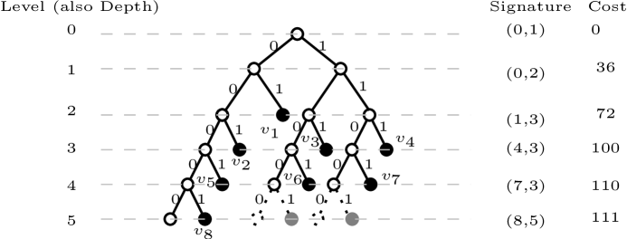
Figure 4: A One-Ended Coding tree for $n=8$ leaves. Note that only $1$-nodes are labelled leaves. On the bottom level, the two dotted $0$-leaves and their two grey $1$-leaf siblings are ‘bad’ nodes added to make the tree full. Signatures and Costs at level $i$ are those of the (truncated) subtree containing the first $i$ levels of the tree. Costs are calculated for $P=\left\{1,2,3,4,5,6,7,8\right\}$.

Our characterization of nodes will be slightly different than in the GMR case. A node in $T^{*}$ will be a good if it’s a $1$-leaf that gets labelled with one of $p_{1},\ldots,p_{n}.$ It will be bad if it is a $0$-node or a $1$-node that doesn’t get lablelled with one of $p_{1},\ldots,p_{n}$.

We will build trees $T^{*}$ from the top-down, level-by-level, At step $i$ our current tree $T$ will be the first $i$ levels of $T^{*}.$ We will identify in $T$ the the number of nodes that are good leaves and the number of nodes, on $T$’s bottom level, that are bad. Note that if $i<\ell(T^{*})$ then, in the next expansion of level, all bad nodes on the current bottom level will become internal, each one contributing one new $1$-node and one new $0$-node on the new bottom level. If $i=\ell(T^{*})$ then $T=T^{*}$ and the bad nodes are extra (those that get labelled with $p_{j},$ $j>n$) $1$-leaves and $0$-leaves on level $i.$

This motivates us to change the definition of signatures and cost as follows:

Definition 12

If $T$ is an $i$-level tree its $i$-level signature is the ordered pair

$$sig_{i}(T)=(m,b)$$

in which

$$m = |\left\{v\in T\,\mid\,\textit{v is a good $1$-leaf, }\ell(v)\leq i\right\}|$$

$$b = |\left\{v\in T\,\mid\,\textit{v is a bad node, }\ell(v)=i\right\}|$$

In the above definition, $b$ is counting leaves in $T$ that, if the tree is expanded one level further, will become internal nodes. Let $T$ be the starting ($0$-level) tree containing only the root. Since the root will always be expanded, it is bad, so $sig_{0}(T)=(0,1).$ This will later be the starting point of our dynamic program.

Let $T$ be an $i$-level tree with $sig_{i}(T)=(m,b)$. The $i$-level partial cost of $T$ is

$$Cost_{i}(T)=\sum_{t=1}^{m}depth(v_{t})\cdot p_{t}+i\cdot\sum_{t=m+1}^{n}p_{t}$$ (14)

As in the GMR case, we want to build an optimal tree $T^{*}$ that satisfies the assumptions. We start by noting that, by assumptions 2(b) and 2(c), the only bad leaves are on the bottom level $\ell=\ell(T^{*}).$

The parents of these bad leaves are on level $\ell-1$ and therefore must be $0$-nodes, since by assumption 2(b), all $1$-nodes on level $\ell-1$ are leaves. From assumption 2(e) there are at most $n-1$ such $0$-internals. So, level $\ell$ contains at most $n-1$ bad 1-leaves and $n-1$ bad $0$-leaves.

Now suppose that $T^{*}$ is being built top-down level-by-level. Let $T$ be the first $i$ levels of $T^{*}$ with $sig_{i}(T)=(m,b)$. By definition $m\leq n.$ Consider the bad nodes on the bottom level of $T.$ If $i<\ell$ then every bad node is internal. From the fullness of the tree, every bad node on level $i$ must have a $1$-leaf descendent in $T^{*}$. There are at most $2n-1$ ($n$ good and $n-1$ bad) $1$-leaves in $T$ and each one can appear at most once in some subtree rooted at level $i$ so $b\leq 2n-1.$ If $i=\ell$ then $b$ is the number of bad leaves in $T^{*}$ which is $\leq 2(n-1).$ We may therefore assume that $b\leq 2n-1.$

This motivates an analogue of Definition 5:

Definition 13

$(m,b)$ is a valid signature if

$$m\leq n\qquad\mbox{and}\qquad b\leq 2n-1$$

We also modify Definition 6:

Definition 14

Let $(m,b)$ be a valid signature. Set $OPT[m,b]$ to be the minimum $i$-level partial cost over all $i$ and all $i$-level trees $T$ with signature $(m,b)$. More precisely

$$OPT[m,b]=min\left\{Cost_{i}(T)\,\mid\,\exists i,T,\textit{T is a i-level tree with}\ sig_{i}(T)=(m,b)\right\}$$ (15)

If no such tree exists, set $OPT[m,b]=\infty.$

Note that if $m=n$, then $OPT[n,b]=\sum_{i=1}^{n}depth(v_{t})\cdot p_{t}$. Thus, from, our previous discussion

$$\min\{OPT^{i}[n,b]\,\mid\,1\leq b\leq 2n-2\}$$

is the cost of the solution to the one-ended coding problem.

Now suppose that $T^{\prime}$ is an $(i-1)$-level tree with $sig_{i-1}=(m^{\prime},b^{\prime}).$ If $T^{\prime}$ is expanded one more level then the $b^{\prime}$ bad nodes on level $i-1$ become internal with each one contributing one $1$-node and one $0$-node to level $i$. Between $0$ and $\min(b^{\prime},n-m^{\prime})$ of the $1$-nodes can become good $1$-leaves. The remaining $1$-nodes and all $b^{\prime}$ $0$-nodes are bad. The newly created $i$-level tree has $sig_{i}(T)=(m,b)$ where

$$m^{\prime}\leq m\leq n,\quad m=m^{\prime}+2b^{\prime}-b,\quad 1\leq b^{\prime}\leq b\leq 2b^{\prime}.$$ (16)

We therefore define expansions as follows:

Definition 15

If $(m^{\prime},b^{\prime}),$ $(m,b)$ are valid signatures that satisfy (16) we write

$$(m^{\prime},b)\rightarrow(m,b).$$

The next few steps exactly follow the development of Lemmas 1, 2, 3 and Corollary 1 with almost identical proofs, so we do not state them explicitly here. The final result is that

$$OPT[m,b]=\min_{{\tiny\{(m^{\prime},b^{\prime})\,\mid\,(m^{\prime},b^{\prime})\rightarrow(m,b)\}}}\Bigl{\{}OPT^{i-1}[m^{\prime},b^{\prime}]+W_{m^{\prime}}\bigr{\}}.$$ (17)

with initial condition $OPT^{0}(0,1)=0$. Note that $(m^{\prime},b^{\prime})\rightarrow(m,b)$ implies either $m^{\prime}<m$ or $m=m$ and $b=2b^{\prime}$. So if $(m^{\prime},b^{\prime})\rightarrow(m,b)$ then $(m^{\prime},b^{\prime})$ is lexicographically smaller than $(m,b)$. Thus, the table can be filled in in lexicographic order to correctly calculate the final values. After filling in the table, the final solution value will be the minimum value of $OPT[n,b],$ where $1\leq b\leq 2n-2$. The actual tree corresponding to this solution can be built by backtracking through the table to find the sequence of expansions

$$(m_{0},b_{0})\rightarrow(m_{1},b_{2})\rightarrow\cdots\rightarrow(m_{i-1},b_{i-1})\rightarrow(n,b)$$ (18)

that corresponds to a min-cost one-ended tree.

The DP table has $O(n^{2})$ entries and each entry requires $O(n)$ time to calculate, leading to an $O(n^{3})$ algorithm for constructing the optimal tree. An algorithm with this running time (based upon a slightly different DP) was given in [10].

We now show that it is possible, using the batching technique earlier introduced for the GMR, to fill in this table in $O(n^{2})$ time. Define

Definition 16

For $1<d$, define

$${\cal I}(d) = \left\{(m,b)\,\mid\,m+b=d,\ 0<b,\ m\leq n\right\},$$

$${\cal I}^{\prime}(d) = \left\{(m^{\prime},b^{\prime})\,\mid\,m^{\prime}+2b^{\prime}=d,\ 0<b,\ m\leq n\right\}.$$

For any fixed $d$ $(m,b)\in{\cal I}(d)$, the definition of $\rightarrow$ implies that

“$(m^{\prime},b^{\prime})\rightarrow(m,b)$”  if and only if  “$(m^{\prime},b^{\prime})\in{\cal I}^{\prime}(d)$ with $b/2\leq b^{\prime}\leq b$”.

Note that if $(m,b)\in{\cal I}^{\prime}(d)$ then $m^{\prime}+b^{\prime}<d$ so $(m^{\prime},b^{\prime})\in{\cal I}(d^{\prime})$ with $d^{\prime}<d$. Also, since $m\leq n$ and $b\leq 2n-1$, we can bound $d\leq 3n-1.$ We may therefore fill in the DP table by filling in all the entries in ${\cal I}(d)$ as a batch in the order $d=2,3,4,\ldots 3n-1$.

We now see that for fixed $d$ we can, by batching, fill in all of the entries in ${\cal I}(d)$ in $O(d)$ time. This will allow filling in the entire table in $O(n^{2})$ time, delivering the promised time reduction.

For fixed $d$ suppose $(m^{\prime},b^{\prime})\in{\cal I}^{\prime}(d)$, i.e., $m^{\prime}+2b^{\prime}=d$. Since $0\leq m^{\prime}$ and $0<b^{\prime}$ we have $1\leq b^{\prime}\leq d/2.$ For such $b^{\prime}$ set

$$\gamma(b^{\prime})=OPT[m^{\prime},b^{\prime}]+W_{m^{\prime}}=OPT[d-2b^{\prime},b^{\prime}]+W_{d-2b^{\prime}}.$$

Note that since $m^{\prime}+b^{\prime}<d$, the values $OPT[m^{\prime},b^{\prime}]$ have already been calculated and can therefore be looked up. Therefore, all of the $\gamma(b^{\prime})$ can be calculated using a total of $O(d)$ time. Then, for $(m,b)\in{\cal I}(d)$,

$$OPT[m,b]=\min\left\{\gamma(b^{\prime})\,\Big{|}\,\frac{b}{2}\leq b^{\prime}\leq b\right\}$$ (19)

Stated this way, this is just a special case of the Range Minimum Query (RMQ) problem.

Given an array $A$ of size $n$, the RMQ problem is to construct a data-structure that, given two indices $i\leq j$, will return the index of a smallest valued item in the subarray $A[i]\ldots A[j].$ There are known algorithms, e.g., [14, 5], for $O(n)$ construction of a data-structure that permits $O(1)$ RMQ queries. In our case, the array is the $b^{\prime}$ indexed set of $\gamma(b^{\prime})$ values. The array has size $O(d)$ and its values can be constructed in $O(d)$ time. [14, 5] then permit us, in $O(d)$ time, to construct an RMQ data structure. Once this structure is constructed, each value $OPT[m,b]$ can be found in $O(1)$ time. Thus, as promised, all of the $OPT[m,b]$ for $(m,b)\in{\cal I}(d)$ can be batched together and evaluated in $O(d)$ time

References

- [1] Julia Abrahams. Code and parse trees for lossless source encoding. Communications in Information and Systems, 1(2):113–146, 2001.
- [2] Alok Aggarwal, Maria M. Klawe, Shlomo Moran, Peter W. Shor, and Robert E. Wilber. Geometric applications of a matrix-searching algorithm. Algorithmica, 2:195–208, 1987.
- [3] Alok Aggarwal, Baruch Schieber, and Takeshi Tokuyama. Finding a minimum-weight -link path in graphs with the concave Monge property and applications. Discrete and Computational Geometry, 12:263–280, 1994.
- [4] M.B. Baer. Reserved-length prefix coding. In Proceedings of the 2008 IEEE International Symposium on Information Theory, pages 2469–2473, July 2008.
- [5] Michael A. Bender, Martin Farach-Colton, Giridhar Pemmasani, Steven Skiena, and Pavel Sumazin. Lowest common ancestors in trees and directed acyclic graphs. J. Algorithms, 57(2):75–94, 2005.
- [6] Toby Berger and Raymond W. Yeung. Optimum -ended binary prefix codes. IEEE Transactions on Information Theory, 36(6):1434–1441, November 1990.
- [7] N. M. Blachman. Minimum cost coding of information. IRE Transactions on Information Theory, PGIT-3:139–149, 1954.
- [8] P. Bradford, M. Golin, L. L. Larmore, and W. Rytter. Optimal prefix-free codes for unequal letter costs and dynamic programming with the monge property. Journal of Algorithms, 42:277–303, 2002.
- [9] R. M. Capocelli, A. De Santis, and G. Persiano. Binary prefix codes ending in a . IEEE Transactions on Information Theory, 40(4):1296–1302, July 1994.
- [10] Sze-Lok Chan and Mordecai J. Golin. A dynamic programming algorithm for constructing optimal “1”-ended binary prefix-free codes. IEEE Transactions on Information Theory, 46(4):1637–1644, 2000.
- [11] Ke-Chiang Chu and John Gill. Mixed-radix Huffman codes. In Ricardo Baeza-Yates and Udi Manber, editors, Computer science: research and applications, pages 209–218, New York, NY, USA, 1992. Plenum Press.
- [12] Shlomi Dolev, Ephraim Korach, and Dmitry Yukelson. The sound of silence: Guessing games for saving energy in mobile environment. In Proceedings of INFOCOM’99, pages 768–775, 1999.
- [13] Sorina Dumitrescu. Faster algorithm for designing optimal prefix-free codes with unequal letter costs. Fundamenta Informaticae, 73(1-2):107–117, 2006.
- [14] Harold N. Gabow and Robert Endre Tarjan. A linear-time algorithm for a special case of disjoint set union. In Proceedings of STOC’83, pages 246–251. ACM, 1983.
- [15] M. Golin and G. Rote. A dynamic programming algorithm for constructing optimal prefix-free codes for unequal letter costs. IEEE Transactions on Information Theory, 44(5):1770–1781, 1998.
- [16] David A. Huffman. A method for the construction of minimum-redundancy codes. In Proceedings of the Institution of Radio Engineers, volume 40, pages 1098–1101, 1952.
- [17] Richard M. Karp. Minimum-redundancy coding for the discrete noiseless channel. IEEE Transactions on Information Theory, 7(1):27–38, 1961.
- [18] Lawrence L. Larmore and Daniel S. Hirschberg. A fast algorithm for optimal length-limited Huffman codes. Journal of the ACM, 37(3):464–473, 1990.
- [19] Baruch Schieber. Computing a minimum weight -link path in graphs with the concave Monge property. Journal of Algorithms, 29(2):204–222, 1998.
- [20] Jan van Leeuwen. On the construction of huffman trees. In Proceedings of the 3rd International Colloquium on Automata, Languages and Programming, pages 382–410, 1976.