Cosmic coincidence problem and variable constants of physics

Abstract

The standard model of cosmology is investigated using time-dependent cosmological constant $\Lambda$ and Newton gravitational constant $G$. The total energy content is described by the modified Chaplygin gas equation of state. It is found that the time-dependent constants coupled with the modified Chaplygin gas interpolate between the earlier matter to the later dark energy dominated phase of the universe. We also achieve a convergence of the parameter $\omega\rightarrow-1$, almost at the present time. Thus our model fairly alleviates the cosmic-coincidence problem which demands $\omega=-1$ at the present time.

Keywords: Chaplygin gas; Coincidence problem; Cosmological constant; Dark energy; Newton’s gravitational constant.

1 Introduction

The astrophysical observations of supernovae of type Ia give a convincing evidence of a universe undergoing an accelerated phase of its expansion history; rather than going to deceleration as was expected theoretically [1, 2, 3, 4]. Similar conclusion has been deduced from the observations of anisotropies in cosmic microwave background by the WMAP [5, 6] which favors a low density, spatially flat ($\Omega_{tot}\sim 1$) universe filled with an exotic vacuum energy containing the maximum portion of the total energy density, $\Omega_{\Lambda}\sim 0.7$ [7]. This mysterious dark energy is represented by a barotropic equation of state (EoS) $p=\omega\rho$, where $p$ and $\rho$ is the pressure and the energy density of dark energy, with $\omega\leq-1$. If $\omega=-1$, it is called ‘cosmological constant’, $-1<\omega<-1/3$ is dubbed ‘quintessence’, while it is called ‘phantom energy’ if $\omega<-1$ [8, 9]. All these candidates have some fundamental problems: The former one presents discrepancy of $120$ orders of magnitude between theoretical and empirical results [10], while quintessence requires fine tuning of cosmological parameters for a suitable choice of the potential function [11]. Also the phantom energy yields eccentric predictions like ‘big rip’ and ripping apart of gravitationally bound objects [12, 13]. Moreover, the variations in $\omega$ suggest that there is no consensus on the actual EoS of dark energy and one can only deal with the upper and lower bounds on $\omega$ [14].

Although the dark energy is generically considered to be a perfect fluid yet it need not to be perfect if it experiences perturbations [15]. Moreover, the dark energy also may not be completely ‘dark’ especially if it gets coupled with matter and energy exchange takes place; consequently the matter evolution becomes modified [16, 17]. It is now obvious that this sudden transition to acceleration from the earlier deceleration phase is rather recent with the corresponding redshift $z\leq 1$ [18]. It has been proposed that the standard model of cosmology may not be sufficient to explain this exotic phenomenon and hence significant modifications are proposed like a modified Friedmann equation $H^{2}\sim g(\rho)$, where $g$ is an arbitrary function of $\rho$ and $H$ is the Hubble parameter [19] and adding a Cardassian term in the Friedmann equation [20]. Other possible explanations proposed are dark energy arising from tachyonic matter [21, 22], van der Waals fluid [23], geometric dark energy [24], Dvali-Gabadadze-Porrati (DGP) gravity model [25] and Randall-Sundrum brane world model [26] are most prominent. Although the nature of dark energy is not clear but its thermodynamical properties suggest a universe filled with it becomes hotter with time [27].

One of the most interesting problems in the present cosmology is the cosmic coincidence (or cosmic conundrum) problem which naively asks: why the energy densities of matter and dark energy are of the same order or the corresponding dimensionless ratio is closer to 1, at current time [28, 29, 30]. This problem can be posed in terms of the EoS parameter $\omega$: if the parameter $\omega\geq-1$ in the past and $\omega<-1$ in the future then why we are observing $\omega=-1$ at present time. In recent years, this problem is addressed using a notion of interacting dark energy model in which both the interacting components i.e. dark energy and matter exchange energy to keep the density ratio close to 1. This model has some intrinsic problems that are still unresolved: the microphysics of energy transfer is not exactly understood i.e. the particles that can mediate the interaction are not pointed out. Moreover, the coupling function (or the decay rate) for the required interaction is chosen quite arbitrarily [31, 32, 33, 34] and also the coupling constant involved is not yet properly constrained theoretically or observationally [35]. In this paper, we address this problem using a simplified approach by considering the constants of physics to evolve over cosmic time. We here take three ansatz for scale factor and analyze the behavior of parameter $\omega$. Curiously, the parameter $\omega(z)$ evolves from positive to negative values and finally converges to $-1$. This result turns out to be consistent with the observations. Hence our model fairly addresses the cosmic coincidence problem and practically alleviates it.

Due to multitude of uncertainties in the determination of $\omega$ observationally and other intrinsic theoretical problems (as discussed above) with it, we here proceed with an EoS commonly called the Chaplygin gas (CG) represented by [36, 37]

$$p=-\frac{X}{\rho},$$ (1)

where $X$ is a constant parameter. The CG effectively explains the evolution of the universe from the earlier deceleration (matter dominated era) to the later acceleration phase (dark energy dominated) as is manifested in the following equation

$$\rho=\sqrt{X+\frac{Y}{a^{6}}}.$$ (2)

Here $Y$ is a constant of integration parameter. For small $a$, it gives $\rho\sim\sqrt{Y}a^{-3}$ while for large $a$, we have $\rho\sim\sqrt{X}$. Therefore models based on CG are also called dark energy-matter unification models [38, 39]. Due to its this effectiveness, several generalizations of CG are proposed (see e.g. [40, 41, 42, 43, 44, 45, 46, 47]). The Chaplygin gas arises from the dynamics of a generalized $d$-brane in a ($d+1,1$) spacetime and can be described by a complex scalar field whose action can be written as a generalized Born-Infeld action [48].

The plan of the paper is as follows: In the second section, we shall present the model of our system. In third section, we determine the cosmological parameters for different choices of the scale factor parameter. The last section is devoted for the conclusion of our paper.

2 The cosmological model with variable constants

The Friedmann-Robertson-Walker (FRW) metric which satisfies the cosmological principle is specified by

$$ds^{2}=-dt^{2}+a^{2}(t)\left[\frac{dr^{2}}{1-kr^{2}}+r^{2}(d\theta^{2}+\sin^{2}\theta d\phi^{2})\right].$$ (3)

Here $a(t)$ is the scale factor that determines the expansion of the universe. Also the parameter $k$ is the curvature parameter determining the spatial geometry of the FRW spacetime. It can take three possible values $k=+1,0,-1$ which correspond to spatially closed, flat and open universe respectively or geometrically spherical, Minkowskian and hyperbolic spacetime respectively.

The equations of motion corresponding to FRW metric are

$$H^{2}\equiv\left(\frac{\dot{a}}{a}\right)^{2} = \frac{8\pi G}{3}\rho+\frac{\Lambda}{3},$$ (4)

$$\frac{\ddot{a}}{a} = -\frac{4\pi G}{3}(\rho+3p)+\frac{\Lambda}{3}.$$ (5)

Above $H$ is the Hubble parameter. Note that we have assumed $k=0$ in the above equations which is favored by the observational data. Here $\Lambda$ is called the cosmological constant with dimensions of $(length)^{-2}$. Note that Eq. (5) shows that accelerated expansion of the universe $\ddot{a}>0$ is possible if the strong energy condition $\rho+3p>0$ is violated and also it is independent of the choice of $k$. The energy conservation equation for the above system is

$$\dot{\rho}+3H(\rho+p)=0.$$ (6)

The cherished constants of physics that describe the universe need not to be constant but can vary with respect to other parameters. For instance, the cosmological constant $\Lambda(t)=\Lambda(t_{o})+(t-t_{o})\dot{\Lambda}(t_{o})+...$ which is constant at zeroth order approximation but is really a time dependent function at higher order approximations. Note that accelerated expansion of the universe follows from $\dot{\Lambda}>0$. The cosmic history of $\Lambda$ shows that it was large in the past while it is small at present and will continue to decrease, hence it gives a parametrization $\Lambda\propto t^{\sigma}$, $\Lambda\propto\rho^{\gamma}$ and $\Lambda\propto H^{2}$ [49, 50]. A variable cosmological constant also arises in theories of higher spatial dimensions like string theory and manifests itself as the energy density for the vacuum [51] and it can also addresses the cosmic age problem effectively [52]. Similarly, there is some evidence of a varying Newton’s constant $G$: Observations of Hulse-Taylor binary pulsar B$1913+16$ gives a following estimate $0<\dot{G}/G\sim 2\pm 4\times 10^{-12}{yr}^{-1}$ [53], helioseismological data gives the bound $0<\dot{G}/G\sim 1.6\times 10^{-12}{yr}^{-1}$ [54] (see Ref [55] for various bounds on $\dot{G}/G$ from observational data). The variability in $G$ results in the emission of gravitational waves. Dimensional analysis also shows that the time dependent parameter $\Lambda$ to be decreasing with time $t$ [56, 57]. In another approach, it is shown that $G$ can be oscillatory with time [58]. It is recently proposed that variable cosmic constants are coupled to each other i.e. variation in one leads to changes in others [59]. A variable gravitational constant also explains the dark matter problem as well [60]. Also discrepancies in the value of Hubble parameter can be removed with the consideration of variable $G$ [61]. Due to these reasons, we shall take $\Lambda$ and $G$ to be time dependent quantities i.e. $\Lambda=\Lambda(t)$ and $G=G(t)$. Hence Eqs. (4) and (5) yield

$$G\dot{\rho}+\rho\dot{G}+3(\rho+p)GH+\frac{\dot{\Lambda}}{8\pi}=0.$$ (7)

Using Eqs. (6) and (7), we can write

$$\rho\dot{G}+\frac{\dot{\Lambda}}{8\pi}=0.$$ (8)

Taking the ansatz for cosmological constant as [62]

$$\Lambda=\frac{3\beta}{\rho^{\gamma}},$$ (9)

where $\beta$ and $\gamma$ are constant parameters. Note that this is a general ansatz and can reduce to Chakraborty and Debnath [63] if $\gamma=-1$. Using the modified Chaplygin gas (MCG) EoS given by [64]

$$p=A\rho-\frac{B}{\rho^{\alpha}},$$ (10)

where $A$ and $B$ are constant parameters and $0\leq\alpha\leq 1$. Thermodynamical analysis of MCG show that the values $\alpha=1/4$ and $B=1/3$ are consistent with the phenomenological results [65]. It is also shown that the recent supernovae data favors $\alpha>1$ values [66, 67]. The MCG reduces to generalized Chaplygin gas (GCG) if $A=0$ while it gives CG if further $\alpha=1$. While a barotropic EoS is obtained if $B=0$. Thus Eq. (10) is a combination of a barotropic and GCG EoS. Precisely, the observations of cosmic microwave background gives the constraint $-0.35\leq A\leq 0.025$ at $95\%$ confidence level [68]. Analysis of various cosmological models show that models based on Chaplygin gas best fit with supernova data [69]. Using Eq. (10) in (6), we get the density evolution of MCG as

$$\rho=\left(x+Ca^{-y}\right)^{\frac{1}{1+\alpha}},$$ (11)

where $x=\frac{B}{1+A}$ and $y=3(1+\alpha)(1+A).$ Making use of Eqs. (9) and (11) in (8), the parameter $G$ is determined to be

$$G=\frac{-3\beta\gamma C}{8\pi(\alpha+\gamma+2)}\left[(x+Ca^{-y})^{-\delta}\left(1+\frac{xa^{y}}{C}\right)^{\delta}{{}_{2}F_{1}}\left(\delta,\delta,1+\delta,-\frac{xa^{y}}{C}\right)\right],$$ (12)

where

$$\delta=\frac{\alpha+\gamma+2}{1+\alpha}.$$ (13)

The parameter $\Lambda$ can alternatively be written as

$$\Lambda=3\beta(x+Ca^{-y})^{\frac{-\gamma}{1+\alpha}}.$$ (14)

3 Determination of cosmological parameters

To analyze the behavior of the above cosmological parameters, we will consider three cases:

1. $a\simeq a_{0}T^{n},$

2. $a\simeq(uT-v)^{\frac{1}{(1+q)}}$,

3. $a\simeq[e^{-DPT}-1]^{-\frac{1}{P}}.$

Here $D$, $P$, $q$, $u$, $v$, $n$ and $a_{o}$ are constant parameters. Also $T=t/t_{o}$ is the dimensionless time parameter with $t_{o}$ is the current age of the universe.

3.1 Power law form of scale factor

We consider power law form of the scale factor

$$a\simeq a_{o}T^{n},$$ (15)

where $a_{o}$ and $n$ are arbitrary constants. For this choice, it is possible to get the accelerated expansion of the universe if $n>1$. Now, all the physical parameters will take the following forms as:

$$\rho \simeq \left(x+\frac{C}{(a_{o}T^{n})^{y}}\right)^{\frac{1}{1+\alpha}},$$ (16)

$$G \simeq \frac{-3\beta\gamma C}{8\pi(\alpha+\gamma+2)}[\left(x+\frac{C}{(a_{o}T^{n})^{y}}\right)^{-\delta}\left(1+\frac{x(a_{o}T^{n})^{y}}{C}\right)^{\delta}$$ (17)

$$\times{{}_{2}F_{1}}\left(\delta,\delta,1+\delta,-\frac{x(a_{0}T^{n})^{y}}{C}\right)],$$

$$\Lambda \simeq 3\beta\left(x+\frac{C}{(a_{o}T^{n})^{y}}\right)^{\frac{-\gamma}{1+\alpha}},$$ (18)

$$p \simeq A\left[\left(x+\frac{C}{(a_{o}T^{n})^{y}}\right)^{\frac{1}{1+\alpha}}\right]-\frac{B}{\left[\left(x+\frac{C}{(a_{o}T^{n})^{y}}\right)^{\frac{1}{1+\alpha}}\right]^{\alpha}}.$$ (19)

The cosmological parameters obtained in this section are plotted in figures 1 to 4 against parameter $T$.

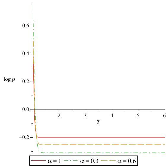
Figure 1: The energy density $\rho$ (see Eq. 16) is plotted against time $T$. Model parameters are fixed at $A=B=C=n=2$, $a_{o}=1$, $\gamma=-0.5$ and $\beta=1$.

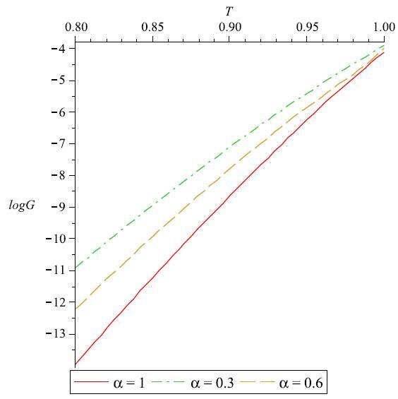
Figure 2: The parameterized Newton’s constant $G$ (see Eq. 17) is plotted against time parameter $T$ for different choices of $\alpha$. Model parameters are fixed as taken in Fig.1

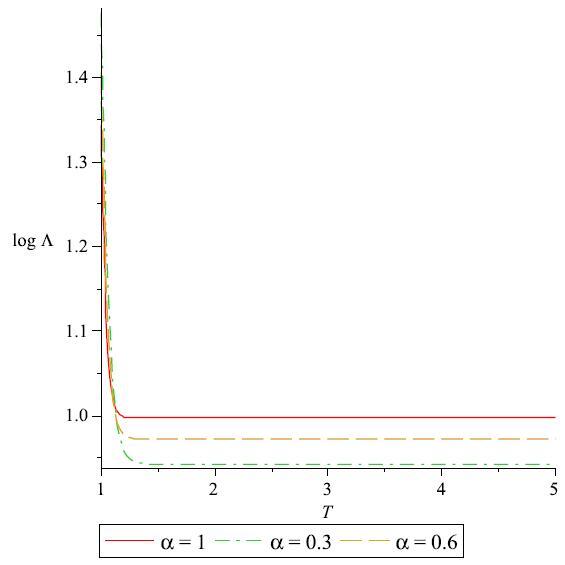
Figure 3: The cosmological constant $\Lambda$ (see Eq. 18) is plotted against time parameter $T$. Model parameters are fixed as taken in Fig.1

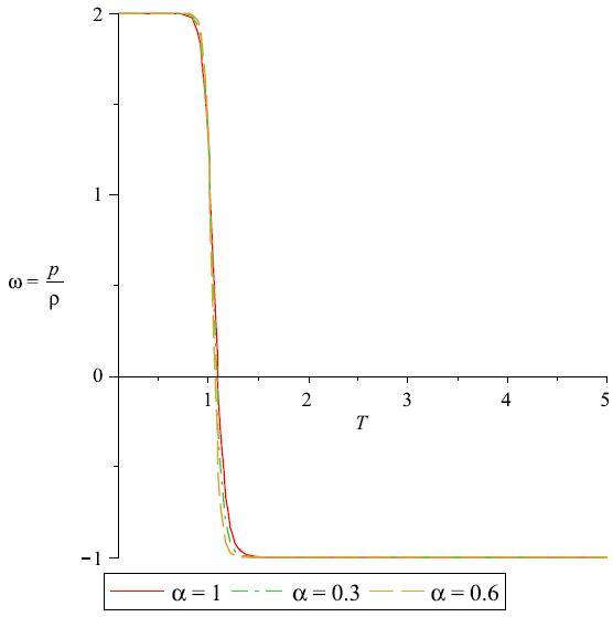
Figure 4: The EoS parameter $\omega=p/\rho$ (see Eq. 16 and 19) is plotted against the time parameter $T$. Model parameters are fixed as taken in Fig.1

3.2 Negative constant deceleration parameter

In this case, we consider constant deceleration parameter model defined by

$$-\frac{\ddot{a}}{aH^{2}}=constant=q.$$ (20)

Here the constant is taken to be negative i.e. it is an accelerating model of the universe [70]. The solution of equation (20) is

$$a\simeq(uT-v)^{\frac{1}{(1+q)}},$$ (21)

where, $u$ and $v$ are integration constants. This equation implies, the condition of expansion is $1+q>0$. Now, all the physical parameters will take the following forms as:

$$\rho \simeq \left(x+\frac{C}{(uT-v)^{\frac{y}{(1+q)}}}\right)^{\frac{1}{1+\alpha}},$$ (22)

$$G \simeq \frac{-3\beta\gamma C}{8\pi(\alpha+\gamma+2)}[\left(x+\frac{C}{(uT-v)^{\frac{y}{(1+q)}}}\right)^{-\delta}\left(1+x\frac{(uT-v)^{\frac{y}{(1+q)}}}{C}\right)^{\delta}$$ (23)

$$\times{{}_{2}F_{1}}\left(\delta,\delta,1+\delta,-x\frac{(uT-v)^{\frac{y}{(1+q)}}}{C}\right)],$$

$$\Lambda \simeq 3\beta\left(x+\frac{C}{(uT-v)^{\frac{y}{(1+q)}}}\right)^{\frac{-\gamma}{1+\alpha}},$$ (24)

$$p \simeq A\left[\left(x+\frac{C}{(uT-v)^{\frac{y}{(1+q)}}}\right)^{\frac{1}{1+\alpha}}\right]-\frac{B}{\left[\left(x+\frac{C}{(uT-v)^{\frac{y}{(1+q)}}}\right)^{\frac{1}{1+\alpha}}\right]^{\alpha}}.$$ (25)

The cosmological parameters obtained in this section are plotted in figures 5 to 8 against parameter $T$.

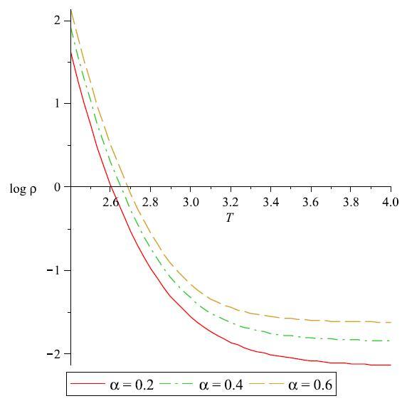
Figure 5: The density parameter $\rho$ (see Eq. 22) is plotted against time $T$. Model parameters are fixed at $A=B=C=0.08$, $u=1$, $v=2$, $q=\gamma=-0.2$ and $\beta=1$.

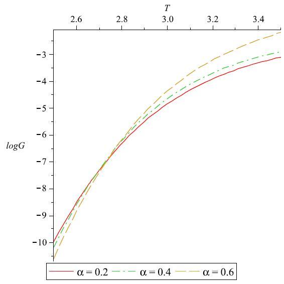
Figure 6: The Newton’s constant $G$ (see Eq. 23) is plotted against time parameter $T$ for different choices of $\alpha$. Other model parameters are fixed as in Fig.5

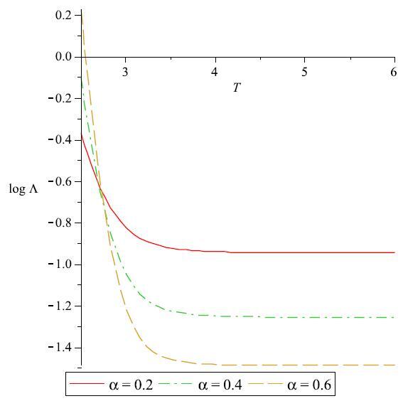
Figure 7: The cosmological constant $\Lambda$ (see Eq. 24) is plotted against time parameter $T$. Other model parameters are fixed as in Fig.5

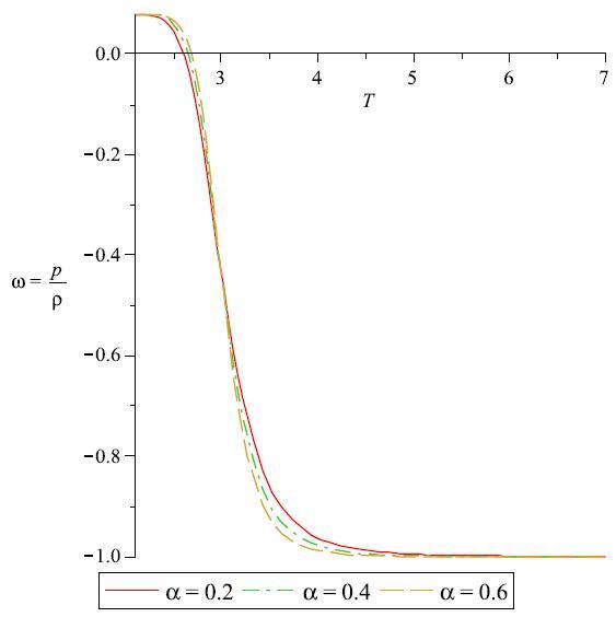
Figure 8: The parameter $p/\rho=\omega$ (see Eq. 22 and 25) is plotted against the time parameter $T$. Other model parameters are fixed as in Fig.5

3.3 Specific form of deceleration parameter

In this case, we consider specific form deceleration parameter model defined by [71]

$$-\frac{\ddot{a}}{aH^{2}}=-1-\frac{Pa^{P}}{1+a^{P}}.$$ (26)

Here $P$ is is a constant. This choice of deceleration parameter provides an early deceleration and late time acceleration of the universe. The solution of equation (26) is

$$a\simeq[e^{-DPT}-1]^{-\frac{1}{P}},$$ (27)

where $D$ is an integration constant. For negative values of $P$, we always get accelerated expansion of the universe. Now, all the physical parameters will take the following forms as:

$$\rho \simeq \left(x+\frac{C}{[e^{-DPT}-1]^{-\frac{y}{P}}}\right)^{\frac{1}{1+\alpha}},$$ (28)

$$G \simeq \frac{-3\beta\gamma C}{8\pi(\alpha+\gamma+2)}[\left(x+\frac{C}{[e^{-DPT}-1]^{-\frac{y}{P}}}\right)^{-\delta}\left(1+x\frac{[e^{-DPT}-1]^{-\frac{y}{P}}}{C}\right)^{\delta}$$ (29)

$$\times{{}_{2}F_{1}}\left(\delta,\delta,1+\delta,-x\frac{[e^{-DPT}-1]^{-\frac{y}{P}}}{C}\right)],$$

$$\Lambda \simeq 3\beta\left(x+\frac{C}{[e^{-DPT}-1]^{-\frac{y}{P}}}\right)^{\frac{-\gamma}{1+\alpha}},$$ (30)

$$p \simeq A\left(x+\frac{C}{[e^{-DPT}-1]^{-\frac{y}{P}}}\right)^{\frac{1}{1+\alpha}}-\frac{B}{\left[\left(x+\frac{C}{[e^{-DPT}-1]^{-\frac{y}{P}}}\right)^{\frac{1}{1+\alpha}}\right]^{\alpha}}.$$ (31)

The cosmological parameters obtained in this section are plotted in figures 9 to 12 against parameter $T$.

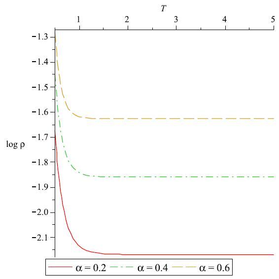
Figure 9: The density parameter $\rho$ (see Eq. 28) is plotted against time $T$. Model parameters are fixed at $A=B=C=0.08$, $P=1.5$, $D=1$ and $\gamma=-0.2$

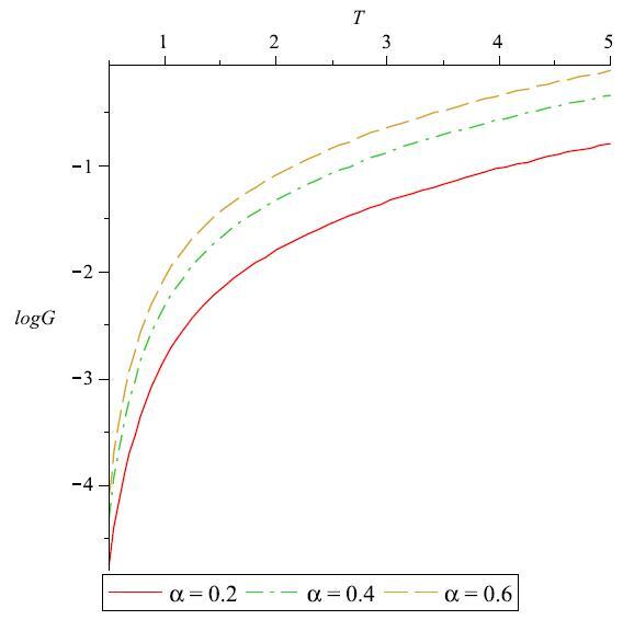
Figure 10: The Newton’s constant $G$ (see Eq. 29) is plotted against time parameter $T$ for different choices of $\alpha$. Other model parameters are fixed as in Fig.9

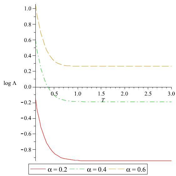
Figure 11: The cosmological constant $\Lambda$ (see Eq. 30) is plotted against time parameter $T$. Other model parameters are fixed as in Fig.9

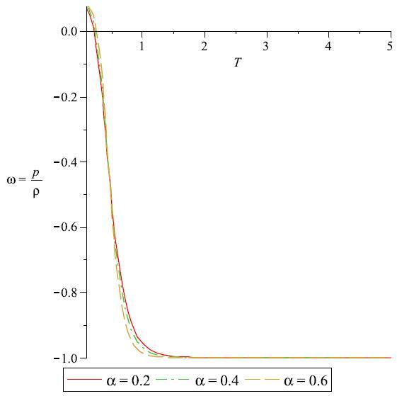
Figure 12: The parameter $p/\rho=\omega$ (see Eq. 28 and 31) is plotted against the time parameter $T$. Other model parameters are fixed as in Fig.9

4 Conclusion and discussion

In this section, we discuss the results of our paper. All the cosmological parameters with the exception of $\omega$ are plotted in figures in 1 to 12 in logarithmic scale against dimensionless time parameter $T$. The parameters in section 3.1 are shown in figures 1 to 4. The cosmological energy density decreases with time and then remains constant in far future. The cosmological constant was large in the past which resulted in inflation while now it is small to produce current accelerated expansion. The Newton’s gravitational constant steadily increased which caused structures to form. Also the dimensionless parameter $\omega$ varies from the positive to negative values and converging to $-1$ at current time $t=t_{o}(\sim 1.2H_{o})$ or $T\simeq 1$ showing that $\omega$ is inherently evolving over cosmic history, with $T=0$ corresponds to the big bang epoch (units are chosen to be meter, kilogram, sec). A similar behavior is obtained for parameters of section 3.2 and 3.3 shown in figures 5 to 8 and 9 to 12, respectively. In figures (13), (14) and (15), we have plotted the same parameters against redshift $z$.

The problem attempted in this paper can also be looked in the context of bulk viscous cosmology. The anisotropic stresses can be important at large scale and hence they should be incorporated in the MCG equation of state (see [72] for the basic formalism). It would also be interesting to extend our model using the modified $f(R)$ gravity theory as well [73].

Acknowledgment

One of us (MJ) would like to thank Asghar Qadir for sharing useful comments on this work. We would also thank the anonymous referee for his useful criticism on this work.

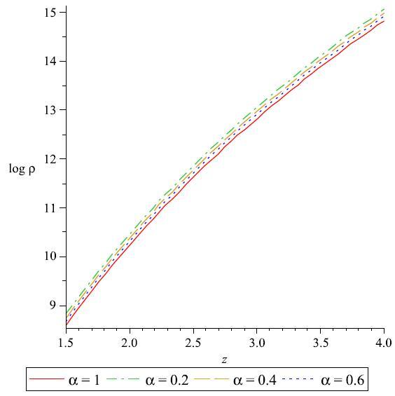
Figure 13: The energy density $\rho$ (see Eq. 16) is plotted against redshift parameter $z$. Model parameters are fixed as in Fig. 13

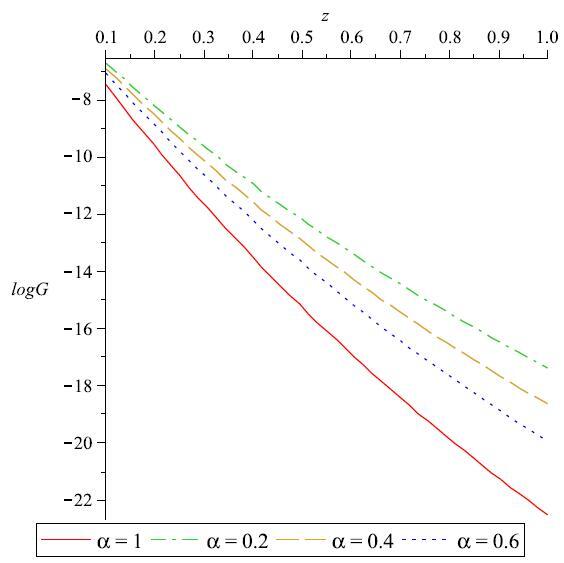
Figure 14: The Newton’s constant $G$ (see Eq. 17) is plotted against redshift parameter $z$. The model parameters are fixed at $A=B=C=2$, $\gamma=-0.2$ and $\beta=1$.

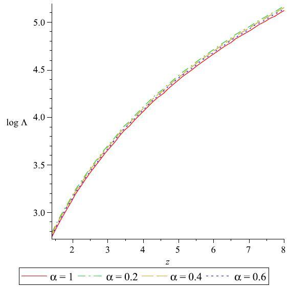
Figure 15: The cosmological constant $\Lambda$ (see Eq. 18) is plotted against redshift parameter $z$. Model parameters are fixed as in Fig. 13

References

- [1] S. Perlmutter et al, Ap. J. 517 (1999) 565.
- [2] A.G. Riess et al, Ast. J. 116 (1998) 1009.
- [3] J.L. Tonry et al, Ap. J. 594 (2003) 1.
- [4] Y. Wang and M. Tegmark, Phys. Rev. Lett. 92 (2004) 241302.
- [5] D.N. Spergel et al, Ap. J. Supp. 148 (2003) 175.
- [6] C.L. Bennett et al, Ap. J. Supp. 148 (2003) 1.
- [7] S. Perlmutter et al, Phys. Rev. Lett. 83 (1999) 670.
- [8] R.R. Caldwell, Phys. Lett. B 545 (2002) 23.
- [9] R.R. Caldwell et al, Phys. Rev. D 73 (2006) 023513.
- [10] V. Sahni, astro-ph/0403324.
- [11] I. Zlatev et al, Phys. Rev. Lett. 82 (1999) 896.
- [12] E. Babichev et al, Phys. Rev. Lett. 93 (2004) 021102.
- [13] M. Jamil et al, Eur. Phys. J. C 58 (2008) 325; astro-ph/0808.1152v1
- [14] A. Upadhye, Nuc. Phys. B (Proc. Suppl.) 173 (2007) 11.
- [15] J.C. Fabris and J. Martin, Phys. Rev. D 55 (1997) 55.
- [16] E.V. Linder, astro-ph/0610173v2.
- [17] S. Nojiri and S.D. Odintsov, hep-th/0505215v4.
- [18] R.A. Daly and S.G. Djogovski, Ap. J. 597 (2003) 9.
- [19] Y. Gong and C.K. Duan, Mon. Not. R. Astron. Soc. 352 (2004) 847.
- [20] K. Freese and M. Lewis, Phys. Lett. B 540 (2002) 1.
- [21] T. Padmanabhan, Phys. Rev. D 66 (2002) 021301.
- [22] P.F. Gonzalez-Diaz, hep-th/0408225v1
- [23] G.M. Kremer, Phys. Rev. D 68 (2003) 123507.
- [24] E.V. Linder, New Astron. Rev. 49 (2005) 93.
- [25] G.R. Dvali et al, Phys. Lett. B 485 (2000) 208.
- [26] L. Randall and R. Sundrum, Phys. Rev. Lett. 83 (1999) 4690.
- [27] J.A.S. Lima and J.S. Alcaniz, Phys. Lett. B 600 (2004) 191.
- [28] S. del Campo et al, Phys. Rev. D 78 (2008) 021302(R).
- [29] N. Dalal et al, Phys. Rev. Lett. 87 (2001) 141302.
- [30] S. Dodelson et al, Phys. Rev. Lett. 85 (2000) 5276.
- [31] M. Quartin et al, astro-ph/0802.0546
- [32] M. Jamil and M.A. Rashid, Eur. Phys. J. C 58 (2008) 111; astro-ph/0802.1146v3
- [33] M. Jamil and M.A. Rashid, Eur. Phys. J. C 56 (2008) 429; astro-ph/0803.3036v3
- [34] M. Jamil, gr-qc/0810.2896v2
- [35] M. Jamil and M.A. Rashid, astro-ph/0802.1144v3
- [36] A. Dev et al, Phys. Rev. D 67 (2003) 023515.
- [37] A. Kamenshchik et al, Phys. Lett. B 511 (2001) 265.
- [38] N. Bili et al, Phys. Lett. B 535 (2002) 17.
- [39] M.C. Bento et al, Phys. Rev. D 70 (2004) 083519.
- [40] S. Chattopadhyay and U. Denath, gr-qc/0805.0070v1.
- [41] U. Debnath, gr-qc/0710.1708v1.
- [42] W. Chakraborty, gr-qc/0711.0079v1
- [43] M.R. Setare, Phys. Lett. B 648 (2007) 329.
- [44] M.R. Setare, Phys. Lett. B 654 (2007) 1.
- [45] Z.K. Guo and Y.Z. Zong, astro-ph/0506091v3.
- [46] A.A. Sen and R.J. Scherrer, Phys. Rev. D 72 (2005) 063511.
- [47] H. Zhang and Z.H. Zhu, astro-ph/0704.3121v2.
- [48] M.C. Bento et al, Phys. Rev. D 66 (2002) 043507.
- [49] U. Mukhopadhay et al, gr-qc/0711.4800v1.
- [50] P.I. Fomin et al, gr-qc/0509042v1.
- [51] H. Liu and P.S. Wesson, gr-qc/0107093v1.
- [52] S. Ray and U. Mukhopadhyay, astro-ph/0411257v2.
- [53] G.S.B. Kogan, gr-qc/0511072v3.
- [54] D.B. Guenther, Phys. Lett. B 498 (1998) 871.
- [55] S. Ray and U. Mukhopadhyay, astro-ph/0510549v1.
- [56] J.A. Belinchon and I. Chakrabarty, gr-qc/0404046v1.
- [57] J.A. Belinchon, gr-qc/809.2412v1.
- [58] A. Pradhan et al, gr-qc/0608107v1.
- [59] R.G. Vishwakarma, gr-qc/0801.2973v1.
- [60] I. Goldman, Phys. Lett. B 281 (1992) 219.
- [61] O. Bertolami et al, Phys. Lett. B 311 (1993) 27.
- [62] A.I. Arbab, hep-th/0711.1465v1.
- [63] W. Chakraborty and U. Debnath, gr-qc/0705.4147v1.
- [64] H. Jing et al, Chin. Phys. Lett. 25 (2008) 347.
- [65] M.L. Bedran et al, Phys. Lett. B 659 (2008) 462.
- [66] O. Bertolami et al, Mon. Not. R. Ast. Soc. 353 (2004) 329.
- [67] M.C. Bento et al, Phys. Rev. D 71 (2005) 063501.
- [68] D.J. Liu and X.Z. Li, astro-ph/0501115v1.
- [69] G. Panotopoulos, Phys. Rev. D 77 (2008) 107303.
- [70] F. Rahaman et al, Astrophys. Space Sci. 299 (2005) 211.
- [71] N. Banerjee and S. Das, astro-ph/0505121.
- [72] M.K. Mak et al, gr-qc/0110119v1.
- [73] P.S. Denath and B.C. Paul, gr-qc/0508031v2.