Abstract

We investigate a modification in the action of inflaton due to noncommutativity leads to a nonstandard initial vacuum and oscillatory corrections in the initial power spectrum. We show that the presence of these oscillations causes a drop in the WMAP $\chi^{2}$ about $\Delta\chi^{2}\sim 8.5$. As a bonus, from the parameter estimation done in this work, we show that the noncommutative parameters can be precisely bound to $10^{16}$ GeV or $10^{4}$ GeV depending on the inflation scale.

1 Introduction

It has recently been emphasized that the effects of trans-Planckian physics might be observable on cosmological scales in the spectrum of Cosmic Microwave Background (CMB) radiation [1]-[18]. An especially intriguing theory that could makes this possible is inflation [19]-[23]. The mechanism of inflation answers several questions that can not be solved in the standard big bang cosmology. It is also the first predictive theory for the origin of structures in the Universe and these predictions have been verified to great accuracy using CMB anisotropy experiments.

The phase of inflation must have lasted about 60 e-foldings so that the observed structures in the Universe had enough time to be seeded from vacuum fluctuations. Consequently it can be possible that inflation is begun from scales with characterized wavelengths much shorter than the Planck length $l_{P}$. Therefore one can trace the trans-Planckian effects on the inflationary predictions. For instance, due to trans-Planckian effects on the vacuum fluctuations, the scale invariant primordial power spectrum $P_{0}$ could be modified to a power spectrum which contains superimposed oscillatory terms suppressed by the scale $\sigma_{n}=(\frac{H}{\Lambda})^{n+1}$ [12, 24, 25, 26]. Here, $H$ is the Hubble scale during inflation and $\Lambda$ is the scale associated with the trans-Planckian physics.

Although the power spectrum and CMB fluctuation can be influenced by the details of high energy scale physics, there is no agreement on the size of these effects and $n$ can be $n=0,1,2$ (see [12, 24, 25, 26]). For example using the low energy effective field theory and general decoupling arguments, Kaloper et al. [26] have shown a suppression of the order of $\sigma_{1}=(\frac{H}{\Lambda})^{2}$ and have discussed that it is too small to be observed during future CMB experiments. This result strongly violates the first conclusions that the deviation would be testable [1, 2]. The argument of [26] has been criticized by some authors [28, 29]. Brandenberger and Martin in [28] have shown that instead of [26], the trans-Planckian physics can leave imprints on the CMB anisotropy. This approach is the same as the Danielsson approach [12]. Both insist on this fact that the vacuum state must be modified due to trans-Planckian physics. Although the preliminary data analysis [30, 31, 32] showed that these oscillatory modifications decrease the WMAP $\chi^{2}$ but recently Groeneboom and Elgaroy, by investigating the Danielsson conclusion [12], have discussed that there is no significant evidence for the simulated data to prefer the trans-Planckian models [33]. We have also analyzed the Danielsson formula and observed no improvement in the $\chi^{2}$.

In this work we change the kinetic part of an inflaton action by assuming a harmonic oscillatory term which comes from noncommutativity to resolve the UV/IR mixing problem. This term plays the role of a barrier potential and makes the vacuum state to be a combination of negative and positive modes. We show that such modification of a vacuum state leads to a power spectrum containing oscillatory corrections similar to the Danielsson result but with an important difference. Using the cosmological Monte Carlo (CosmoMC) code, we will show that due to the presence of this difference, our model gives a drop in the $\chi^{2}$ in spite of the Groeneboom and Elgaroy’s negative conclusion. Having parameters estimated by CosmoMC, the noncommutativity scale $\Lambda_{NC}$ is determined as a function of inflation scale $H$. Knowing a variety of bounds on $H$, we find the scale of noncommutativity to be of the order of $10^{16}$ GeV or of the order of $10^{4}$ GeV depending on what scales for inflation are used.

The paper is organized as follows. In sections 2 and 3 we briefly review the standard calculation of the inflationary power spectrum when the trans-Planckian effects are taken into account. In section 4 we derive our modified formula for the power spectrum when an extra term is added to the free part of inflaton action due to noncommutativity. Comparison of our theoretical predictions with the WMAP data is given in section 5. In this section we bound the noncommutative scale using parameters estimated by CosmoMC.

2 Initial Vacuum State

The authors of [28] have suggested that the evolution of the inflaton modes can be separated into three phases I, II and III shown in Figure 1. During phase I, the physical wavelength $\lambda$ of modes is smaller than the scale $\Lambda\approx l_{P}$ and the effects of short distance physics are expected to be important. During phase II, the physical wavelength is larger than the Planck scale but smaller than the Hubble radius $H^{-1}$. Since during phase II the background is time-dependent, there is a nontrivial mixing between creation and annihilation operators at different times[34]. This kind of mixing takes place via Bogoliubov transformation which through it a mode $v(\eta)$ must be a linear combination of positive and negative frequency initial modes[34]

$$v(\eta)=\alpha_{k}v^{(in)}_{k}(\eta)+\beta_{k}v^{(in)\ast}_{k}(\eta)$$ (1)

where $\alpha_{k}$ and $\beta_{k}$ are the Bogoliubov coefficients which satisfy the normalization condition

$$|\alpha_{k}|^{2}-|\beta_{k}|^{2}=1$$ (2)

Finally in region III, modes cross the Hubble radius $H^{-1}$ and squeeze.

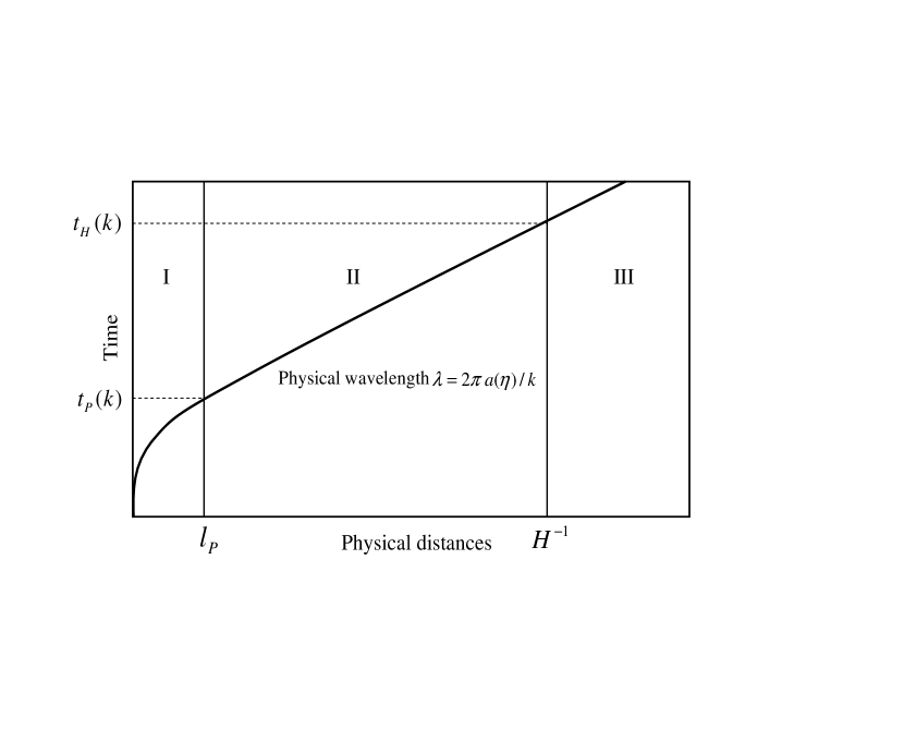
Figure 1: Periods

The coefficients $\alpha_{k}$ and $\beta_{k}$ are determined by matching (1) to the vacuum state. But in any expanding universe such as inflationary period, the notion of a vacuum is ambiguous [34]. The reason is that $H$ is time-dependent during inflation and so inflating space-time is not exactly a de Sitter space-time in which defining vacuum state is possible. This is a well-known problem in curved space-times where the concept of the vacuum state is quite ambiguous due to the absence of Killing vector fields [34].

A space-time such as de Sitter space-time, admits a timelike Killing vector field, then this provides a natural way to distinguish positive and negative frequency modes and then similar to the standard procedure in Minkowski space, associate these distinguished modes with annihilation and creation operators. By definition, the vacuum state of a de Sitter space-time, (known as the Bunch-Davies vacuum [35]), will be the state that is annihilated by all the annihilation operators. This vacuum state is invariant under the symmetry group of the space-time. For inflationary theories although $H$ is time dependent and consequently the Killing vector cannot be defined, this ambiguity can be ignored by choosing the adiabatic vacuum when the wavelength of a mode is much shorter than the curvature scale of space-time. This vacuum is known as the adiabatic vacuum [34].

In addition to this, there is also an extra ambiguity as the result of trans-Planckian physics below the certain cut-off $\Lambda$ through which the vacuum is ambiguous since the physics of region I (Planck scales) is unknown. Danielsson approach [12] tries to solve this kind of ambiguity. In this approach there is no explicit assumption about the trans-Planckian physics of region I and the emphasize is made only on the point that the wavefunctions of the fluctuation modes are not in their vacuum states when they enter into phase II [12]. Then for avoiding the ambiguity of region I which is the region of unknown physics, one defines the vacuum at the time $\eta_{0}$ when the physical momentum $p$ of a mode equals the scale of new physics i.e. $\Lambda$ [12]. The physical momentum $p$ and the comoving momentum $k$ are related through

$$k=ap=-\frac{p}{\eta H}.$$ (3)

By imposing the initial conditions when $p=\Lambda$, we find the conformal time $\eta_{0}$ as

$$\eta_{0}=-\frac{\Lambda}{Hk}.$$ (4)

Without knowledge of the physics beyond the scale $\Lambda$, in order to choose the vacuum it is not necessary to take the limit $\eta_{0}\rightarrow\infty$ but instead one had to stop at the value of conformal time given by (4). So the question about the trans-Planckian physics is that of choosing the vacuum state which clearly would be different from the adiabatic or Bunch-Davies vacuum. An alternative vacuum leads to the corrections of order $\sigma_{n}=(\frac{H}{\Lambda})^{n+1}$ in the power spectrum.

3 Region II

In this section we recall what happens in region II during the inflation. During inflation the action of the massless scalar inflaton field $\varphi$ minimally coupled to gravity is written as [19]-[23]

$$S=\int\>d^{4}x\>\sqrt{-g}\left(\frac{1}{2}g^{\mu\nu}\partial_{\mu}\varphi\partial_{\nu}\varphi-V(\varphi)\right)$$ (5)

where $g^{\mu\nu}$ is metric and $V(\varphi)$ is the inflaton potential. Usually one assumes a spatially flat, homogeneous and isotropic background with the metric

$$ds^{2}=a^{2}(\eta)\left(d\eta^{2}-d\textbf{x}\cdot d\textbf{x}\right)$$ (6)

where $\eta$ is the conformal time and $a(\eta)$ is the scale factor. Here we restrict our attention to the scalar perturbations in metric which will be gauge dependent. Hence the line element in the longitudinal gauge, takes the form

$$ds^{2}=a^{2}(\eta)\left[(1+2\Phi(\eta,\textbf{x}))d\eta^{2}-(1-2\Psi(\eta,\textbf{x}))d\textbf{x}\cdot d\textbf{x}\right]$$ (7)

where the space-time dependent functions $\Phi$ and $\Psi$ are the two physical metric degrees of freedom which describe the scalar metric fluctuations. In the absence of anisotropic stress, the two metric perturbation $\Phi$ and $\Psi$ coincide, $\Phi=\Psi$. During inflation the inflaton field can be separated into a classical background and a fluctuating part

$$\varphi(\eta,\textbf{x})=\varphi_{0}(\eta)+\delta\varphi(\eta,\textbf{x})$$ (8)

Because of the Einstein equation, the metric fluctuation $\Phi$ is determined by the matter fluctuation $\delta\varphi$. Thus every thing can be reduced to the study of a single gauge-invariant variable field [25, 28]

$$v=a\left(\delta\varphi+\frac{\varphi_{0}}{\mathcal{H}}\Phi\right)\equiv z\mathcal{R},$$ (9)

where $a^{\prime}=da/d\eta$, $\mathcal{H}=\frac{a^{\prime}}{a}$, $z\equiv a\frac{\varphi^{\prime}_{0}}{\mathcal{H}}$ and $\mathcal{R}$ denote the curvature perturbation in comoving gauge [25, 28]. It is convenient to work with the variable $\mu_{s}$ defined by $\mu_{s}\equiv-\sqrt{2\kappa}v$ where $\kappa=8\pi/m_{P}$. After quantizing the theory, in the Schrödinger picture, we can write $\mu_{s}(\eta,\textbf{x})$ as

$$\mu_{s}(\eta,\textbf{x})=\frac{1}{(2\pi)^{\frac{3}{2}}}\int d^{3}k\>\left[\>U^{II}_{k}(\eta)\>\hat{a}_{k}\>e^{i\textbf{k}\cdot\textbf{x}}\>+\>U^{II\>\ast}_{-k}(\eta)\>\hat{a}^{{\dagger}}_{-k}\>e^{-i\textbf{k}\cdot\textbf{x}}\>\right],$$ (10)

where $\hat{a}_{k}$ and $\hat{a}^{{\dagger}}_{-k}$ are respectively the creation and annihilation operators. The evolution of $U^{II}_{k}(\eta)$ is given by the Klein-Gordon equation of motion in Fourier space

$$U^{II\>^{\prime\prime}}_{k}(\eta)+\left(k^{2}-\frac{z^{\prime\prime}}{z}\right)U^{II}_{k}(\eta)=0.$$ (11)

In the case of slow-roll inflation limit the quantity $\frac{z^{\prime\prime}}{z}$ is reduced to [25]

$$\frac{z^{\prime\prime}}{z}\sim\frac{2+3\epsilon}{\eta^{2}},$$ (12)

in which $\epsilon$ is the slow roll parameter. The general solution for $U^{II}_{k}(\eta)$ is written in the form

$$U^{II}_{k}(\eta)=\frac{\sqrt{\pi}}{2}\left|\eta\right|^{\frac{1}{2}}\left(\>\alpha_{k}\>e^{-\frac{i\pi}{2}(\frac{1}{2}-\nu)}\>H_{\nu}(|k\eta|)+\beta_{k}\>e^{\frac{i\pi}{2}(\frac{1}{2}-\nu)}\>H^{\ast}_{\nu}(|k\eta|)\>\right),$$ (13)

where $H_{\nu}$ is the Henkel function of the first kind. In the above expression, $\nu$ is a function of $\epsilon$ in the slow roll case. The coefficients $\alpha_{k}$ and $\beta_{k}$ are the Bogoliubov coefficients which are fixed by the initial condition. Using the asymptotic form of the Hankel functions in the limit $k\eta\gg 1$[37]

$$H^{(1)}_{\nu}(k\eta\gg 1)\approx\sqrt{\frac{2}{\pi}|k\eta|}e^{i(k\eta-\pi\frac{\nu}{2}-\frac{\pi}{4})},$$ (14)

one can find the leading behavior of $U^{II}_{k}(\eta)$

$$U^{II}_{k}(\eta)\approx\frac{\alpha_{k}}{\sqrt{2k}}\>e^{-ik(\eta-\eta_{0})}+\frac{\beta_{k}}{\sqrt{2k}}\>e^{ik(\eta-\eta_{0})}+\cdot\cdot\cdot.$$ (15)

Naively, one can choose a boundary initial condition by simply stating that the modes in the limit $\eta\rightarrow-\infty$ are positive frequency modes of the kind of Bunch-Davis vacuum which leads to $\alpha=1$ and $\beta=0$. But as have been widely discussed recently [1, 2, 3], [7]-[18], by the trans-Planckian considerations, the vacuum state is not a Bunch-Davis one. To solve this ambiguity, Danielsson [12] assumed the following boundary condition

$$\frac{d}{d\eta}\left(U^{II}_{k}/a\right)(\eta_{0})=-ik\left(U^{II}_{k}/a\right)(\eta_{0})$$ (16)

which gives the coefficients $\alpha$ and $\beta$ and consequently the power spectrum $P(k)$ as

$$P(k)=P_{0}(k)\left(1+\xi\left(\frac{k}{k_{0}}\right)^{-\epsilon}\sin\left[\frac{2}{\xi}\left(\frac{k}{k_{0}}\right)^{\epsilon}+\phi\right]\right),$$ (17)

where $\xi\equiv\frac{H}{\Lambda}$ and $\phi$ is a phase factor. A similar result reported in [38] and also see [39] and [40] for another discussion and conclusion. In the following section we will drive such a formula for trans-Planckian power spectrum by considering an assumption about the physics in the region $I$ instead of boundary condition (16). Our result for the power spectrum will be different from (17) and the difference is that in our case two coefficients $\xi_{1}$ and $\xi_{2}$ appear instead of $\xi$.

4 Region I

Since in region I the complete theory of quantum gravity is still unknown, one way to tackle with it is to work with effective scenarios. For instance, it is possible to include the higher dimensional terms to the Lagrangian [26, 29, 36] or invoke the modified dispersion relation models [28]. Another possibility that has been greatly studied in recent years is the noncommutativity of space-time [3]. Noncommutative space-time emerges in string theory configuration and is an effective picture of the foamy space-time above the energy scale $\Lambda_{NC}$ (for review see [41, 42]). Field theories on a noncommutative space-time

$$\left[\>\hat{x}^{\mu},\>\hat{x}_{\nu}\>\right]=i\theta_{\mu\nu}$$ (18)

are defined by replacing the ordinary product of fields by the star product [43, 44]

$$\phi_{1}\star\phi_{2}(x)=\int\frac{d^{d}kd^{d}q}{(2\pi)^{d}}\tilde{\phi}_{1}(k)\tilde{\phi}_{2}(q)e^{ik_{\mu}\theta^{\mu\nu}q_{\nu}}e^{i(k+q)x}\;,$$ (19)

where the $\theta_{\mu\nu}$ is a real antisymmetric tensor which introduce a scale $\Lambda_{NC}=\frac{1}{\sqrt{\theta}}$. In Eq. (19) the tilde denotes the Fourier transform. Because of this star-product, a puzzling mixing of UV and IR scales known as UV/IR mixing appeared during performing loop calculations in noncommutative field theories [45]. The UV/IR mixing makes theories nonrenormalizable. Several attempts have been done in order to solve this problem [46, 47, 48]. For the case of scalar theories, Grosse and Wulkenhaar in [46], have shown that one can cancel out the UV/IR mixing problem by introducing a modification in the free part of the action. They assume a harmonic oscillatory term to the action such that the kinetic term becomes

$$S_{kin}[\phi]=\int\>d^{4}x\left(\>\frac{1}{2}\partial_{\mu}\phi\partial^{\mu}\phi+\frac{\Omega^{2}}{2}\tilde{x}^{2}\phi^{2}\right),$$ (20)

where $\Omega\in(\>0,1]$ and $\tilde{x}_{\mu}=2\theta^{-1}_{\mu\nu}x^{\nu}$. Furthermore in (20), for the case of $\Omega^{2}=1$ the action is expected to enjoy a duality transformation between position and momentum [49]

$$\hat{\phi}(p) \leftrightarrow\pi^{2}\sqrt{|\det\theta|}\;\phi(x)\;, p_{\mu} \leftrightarrow\tilde{x}_{\mu}\;,$$ (21)

where $\hat{\phi}(p_{a})=\int d^{4}x\;\mathrm{e}^{(-1)^{a}ip_{a,\mu}x_{a}^{\mu}}\phi(x_{a})$.

Inspired by this modification, we suggest that the kinetic term of an inflaton action must be modified due to quantum properties of space-time on the scales where trans-Planckian effects become important. Since the noncommutativity is one of effective pictures of the trans-Planckian physics, hence for the inflatons, a modified action such as (20) is considered. Therefor we consider the harmonic oscillator term $\frac{\Omega^{2}}{2}\varphi(x)\tilde{x}^{2}\varphi(x)$ as a correction to the kinetic part of the inflaton action (5), in region I. The noncommutative parameter $\theta_{\mu\nu}$ is also restricted to the following special case where as the result of it the equation of motion of the inflaton is simplified

$$\theta_{\mu\nu}=\left(\begin{array}[]{cccc}0&0&0&\theta\\ 0&0&\theta&0\\ 0&-\theta&0&0\\ -\theta&0&0&0\\ \end{array}\right)$$ (22)

Consequently under this assumption, $\tilde{x}^{2}$ is given by

$$\tilde{x}^{2}=\left(2\>\theta^{-1}_{\mu\nu}x^{\nu}\right)^{2}=4\frac{a^{2}}{\theta^{2}}\left[(x^{3})^{2}-(x^{1})^{2}-(x^{2})^{2}-(\eta)^{2}\right]$$ (23)

and the kinetic part of the inflaton action is written as

$$S_{\mathrm{kin}}=\int\>d^{4}x\>\sqrt{-g}\left(\frac{1}{2}\>g^{\mu\nu}\partial_{\mu}\varphi\>\partial_{\nu}\varphi\>+\>2\>\frac{a^{2}}{\theta^{2}}\left[(x^{3})^{2}-(x^{1})^{2}-(x^{2})^{2}-(\eta)^{2}\right]\varphi^{2}\right).$$ (24)

Now the variable $\mu_{s}(\eta,\textbf{x})$ is decomposed into the Fourier modes in the following general form

$$\mu_{s}(\eta,\textbf{x})=\frac{1}{(2\pi)^{\frac{3}{2}}}\int[d\textbf{k}]\big{(}\>\hat{a}_{k}\>U_{k}(\eta)\>V_{k}(\textbf{x})\>+\>\hat{a}^{{\dagger}}_{k}\>U^{\ast}_{k}\>V^{\ast}_{k}(\textbf{x})\>\big{)}\;,$$ (25)

where $[d\textbf{k}]$ is the measure of the integral and the $V_{k}(\textbf{x})$ is the eigenfunction of the three dimensional Laplace operator $\Delta_{3}$

$$\>\left(\Delta_{3}+(x^{3})^{2}-(x^{2})^{2}-(x^{1})^{2}\>\right)V_{k}(\textbf{x})\!\!\!\!\!\!\! =\frac{1}{\sqrt{-g}}\>\partial_{i}\left(\sqrt{-g}g^{ij}\partial_{j}\right)V_{k}(\textbf{x})$$ (26)

$$\>\>\>\>\>+\left((x^{3})^{2}-(x^{2})^{2}-(x^{1})^{2}\right)\>V_{k}(\textbf{x})$$

$$=k^{2}V_{k}(\textbf{x})\;,$$

in which the metric $g^{ij}$ has been defined in (6) and $k^{2}$ is the eigenvalue. Also in the expansion (25), $U_{k}(\eta)$ obeys the following equation

$$U^{\prime\prime}_{k}(\eta)+\left[\left(k^{2}-\frac{a^{\prime\prime}}{a}\right)+\frac{2}{\theta^{2}}\eta^{2}\right]U_{k}(\eta)=0.$$ (27)

In the case of the absence of the second term in equation (26), the $V_{k}(\textbf{x})$ are simply plane-wave $e^{i\textbf{k}\cdot\textbf{x}}$ and the integration measure in (25) for this case is $\int[d\textbf{k}]=\int d^{3}k$. The differential equation (26) can be solved by separating $V_{k}(\textbf{x})$ into

$$V_{k}(\textbf{x})=V_{k_{3}}(x_{3})V_{k_{1},k_{2}}(x_{1},x_{2})$$ (28)

The differential equation for the $V_{k_{3}}(x_{3})$ reduces to the harmonic oscillator differential equation, which its solution is given in terms of Hermite polynomials. Thus, the wave number $k_{3}$ takes discrete values which we label by positive integers $k\geq 1$. Also for the $V_{k_{1},k_{2}}(x_{1},x_{2})$ we find a differential equation, which its solution is known as parabolic cylinder functions [37]. The parabolic cylinder function, $D_{p}(z)$ with continues $p$, is a class of special functions defined as the solution to the following differential equation

$$\frac{d^{2}D_{p}(z)}{dz^{2}}+\left(\>z^{2}+\lambda(p)\>\right)D_{p}(z)=0,$$ (29)

together with the integral representation as

$$D_{p}(z)=\frac{e^{\frac{-z^{2}}{4}}}{\Gamma(-p)}\>\int_{0}^{\infty}e^{-xz-\frac{x^{2}}{2}}x^{-p-1}dx\>\>\>\>\>\>\>\>\>\>\>\>(\mathrm{Re\>p<0}).$$ (30)

Since $k_{3}$ is discrete and $k_{1}$ and $k_{2}$ are continuous, the integration measure in (25) is given by

$$\int[d\textbf{k}]=\int_{0}^{\infty}\int_{0}^{\infty}d^{3}k_{1}d^{3}k_{2}\sum_{k_{3}=1}^{\infty}.$$ (31)

Because the modes are in region I, one expects $\frac{a^{\prime\prime}}{a}\rightarrow 0$ for the time-dependent part of modes in (27). Hence equation (27) is simplified to

$$U^{\prime\prime}_{\kappa}(\tau)+\big{(}\kappa^{2}+\tau^{2}\big{)}U_{\kappa}(\tau)=0\;,$$ (32)

in which $U_{k}(\eta)$, $\eta$ and $k$ have been redefined as follows,

$$U_{\kappa}(\tau)=\left(\frac{\sqrt{2}}{\theta}\right)^{\frac{1}{4}}U_{k}(\eta),\>\>\>\>\>\>\>\>\>\>\>\tau=\frac{(2)^{\frac{1}{4}}}{\sqrt{\theta}}\eta,\>\>\>\>\>\>\>\>\>\>\>\kappa^{2}=\sqrt{2}\theta k^{2}.$$ (33)

The time evolution of modes in (32) is equivalent to the following situation. Consider a scalar inflaton on a non-static background

$$ds^{2}=C(\eta)\big{(}d\eta^{2}-d\textbf{x}\cdot d\textbf{x}\big{)}.$$ (34)

It can be shown that with a conformal scale factor representing a bouncing universe

$$C(\eta)=a^{2}+b^{2}\eta^{2}\>\>\>\>\>\>\>\>-\infty<\eta<\infty,$$ (35)

one obtains the same equation for the evolution of time-dependent modes [34]. The exact solution to the equation (32) is then given in terms of parabolic cylinder functions [37]

$$U^{I}_{\kappa}(\tau)\equiv U_{\kappa}(\tau)=D_{-\frac{1+i\kappa^{2}}{2}}(\>(1+i)\tau\>).$$ (36)

Now we study the asymptotic behavior of $U^{I}_{\kappa}(\tau)\equiv U_{\kappa}(\tau)$ modes living in region I in order to match them with $U^{II}_{\kappa}(\tau)$ modes living in region II at the boundary $\eta_{0}$. This helps us to obtain coefficients $\alpha_{k}$ and $\beta_{k}$. The parabolic cylinder function $D_{p}(z)$ has the following linear relation [37]

$$D_{p}(z)=e^{-p\pi i}\>D_{p}(-z)\>+\>\frac{\sqrt{2\pi}}{\Gamma(-p)}\>e^{-\frac{(p+1)\pi i}{2}}\>D_{-p-1}(iz)\;,$$ (37)

where $z=(1+i)\tau$ and $p=-\frac{1+i\kappa^{2}}{2}$. This relation is a useful relation in order to rewrite the modes $U^{I}_{\kappa}(\tau)$ as a combination of positive and negative modes. The asymptotic behavior of $D_{p}(z)$ for the large values of $p$ is [37]

$$D_{p}(z)\approx\frac{2^{\frac{-1}{4}+\frac{p}{2}}}{\left(8(-\frac{1}{4}-\frac{p}{2})\right)^{\frac{1}{4}}}\>\exp\left(\left(\frac{1}{4}+\frac{p}{2}\right)\ln\left(\frac{1}{4}-\frac{p}{2}\right)-2\sqrt{-\left(\frac{1}{4}+\frac{p}{2}\right)\frac{z^{2}}{2}}\>\right).$$ (38)

Substituting (38) into the relation (37) with $p=-\frac{1+i\kappa^{2}}{2}$, we find

$$D_{-\frac{1+i\kappa^{2}}{2}}((1+i)\tau)\approx \!\!\!\!\!\!\!\!\frac{2^{-\frac{i\kappa^{2}}{4}}\>e^{\left(\frac{1}{2}+\frac{i\kappa^{2}}{4}\right)\pi i-i\frac{\kappa^{2}}{4}\ln\frac{i\kappa^{2}}{4}}}{\left(2e^{\frac{i\pi}{2}}\kappa^{2}\right)^{\frac{1}{4}}}\>e^{-i\kappa\tau}$$ (39)

$$\!\!\!\!\!\!\!\!\!\!+\frac{\sqrt{2\pi}}{\Gamma\left(\frac{1}{2}+i\frac{\kappa^{2}}{2}\right)}\frac{2^{\frac{i\kappa^{2}}{4}}\>e^{\left(\frac{1}{2}-\frac{i\kappa^{2}}{4}\right)\frac{-\pi i}{2}+i\frac{\kappa^{2}}{4}\ln\frac{-i\kappa^{2}}{4}}}{\left(2e^{\frac{-i\pi}{2}}\kappa^{2}\right)^{\frac{1}{4}}}\>e^{i\kappa\tau}$$

$$\!\!\!\!\!\!\!\!\!\!\!\!\!\approx\frac{i}{(2\kappa^{2})^{\frac{1}{4}}}\exp\left(-\frac{i\pi}{8}-\frac{\kappa^{2}\pi}{2}\right)\>e^{-i\kappa\tau}$$

$$\!\!\!\!\!\!\!\!\!\!-\frac{i\sqrt{2\pi}}{\Gamma\left(\frac{1}{2}+i\frac{\kappa^{2}}{2}\right)(2\kappa^{2})^{\frac{1}{4}}}\exp\left(\frac{i3\pi}{8}-\frac{\kappa^{2}\pi}{4}\right)\>e^{i\kappa\tau}.\>$$

Thus $U^{I}_{k}(\eta)$ can be written as

$$U^{I}_{k}(\eta)\approx\frac{1}{\sqrt{2k}}\>\alpha_{k}\>e^{-ik\eta}+\frac{1}{\sqrt{2k}}\>\beta_{k}\>e^{ik\eta},$$ (40)

where the coefficients $\alpha_{k}$ and $\beta_{k}$ are found by matching the solution (39) with $U^{II}_{k}(\eta)$ in (15) at $\eta=\eta_{0}$ as

$$\alpha_{k}=ie^{-\frac{i\pi}{8}-\frac{k^{2}\pi\theta}{2\sqrt{2}}}e^{ik\eta_{0}},$$ (41)

and

$$\beta_{k}=\frac{-i\sqrt{2\pi}}{\Gamma\left(\frac{1}{2}+i\frac{\theta k^{2}}{2\sqrt{2}}\right)}\>e^{-\frac{3\pi i}{8}-\frac{k^{2}\pi\theta}{4\sqrt{2}}}e^{-ik\eta_{0}}.$$ (42)

Using the identify [37]

$$\left|\Gamma\left(\frac{1}{2}+iy\right)\right|^{2}=\frac{\pi}{\cosh\pi y}$$ (43)

one can verify the normalization relation

$$|\alpha|^{2}-|\beta|^{2}=1$$ (44)

In general the gamma function can be represented in the following form

$$\Gamma\left(\frac{1}{2}+ik^{2}\theta\right)=\left|\Gamma\left(\frac{1}{2}+ik^{2}\theta\right)\right|\>e^{i\varphi(k^{2}\theta)}=\frac{\sqrt{\pi}}{\cosh^{1/2}\pi k^{2}\theta}\>e^{i\varphi(k^{2}\theta)}\;,$$ (45)

where $\varphi(k^{2}\theta)$ is a phase factor. We will employ this relation for the next calculations of $P(k)$.

Using equations (41) and (42), one can calculate the corresponding energy density and pressure by the mean value of energy-momentum tensor $\left<T_{\mu\nu}\right>$ in the trans-Planckian region [27]

$$\left<\rho\right>=\frac{1}{4\pi^{2}a^{4}}\int dkk^{2}\left(a^{2}\left|\left(\frac{U_{k}^{I}}{a}\right)^{\prime}\right|^{2}+k^{2}\left|U_{k}^{I}\right|^{2}\right)$$ (46)

$$\left<p\right>=\frac{1}{4\pi^{2}a^{4}}\int dkk^{2}\left(a^{2}\left|\left(\frac{U_{k}^{I}}{a}\right)^{\prime}\right|^{2}-\frac{k^{2}}{3}\left|U_{k}^{I}\right|^{2}\right)$$ (47)

Inserting the mode function $U_{k}^{I}(\eta)$ into the vacuum expressions of the energy density and pressure and using the normalization condition (44), one finds

$$\left<\rho\right>=\frac{1}{4\pi^{2}a^{4}}\int dkk^{3}\left|\beta_{k}\right|^{2}$$ (48)

$$\left<p\right>=\frac{-1}{4\pi^{2}a^{4}}\int dkk^{3}\left(\frac{2}{3}+\frac{1}{3}\left|\beta_{k}\right|^{2}\right)$$ (49)

in the trans-Planckian region. Now at this stage we turn to the superhorizon scales ($k\eta\ll 1$) and start to compute the power spectrum. First we substitute (41) and (42) in (13) and take the superhorizon limit. Since in this limit the Hankel functions take the following form

$$H_{\nu}(k\eta\ll 1)\approx\sqrt{\frac{2}{\pi}}\>e^{-i\frac{\pi}{2}}2^{\nu-\frac{3}{2}}\frac{\Gamma(\nu)}{\Gamma(\frac{3}{2})}(k\eta)^{-\nu}$$ (50)

The amplitude of $U^{II}_{k}$ modes is given by

$$|U^{II}_{k}|\approx\frac{2^{\nu-\frac{3}{2}}}{\sqrt{2k}}\frac{\Gamma(\nu)}{\Gamma(\frac{3}{2})}\>|\alpha_{k}+\beta_{k}|(k\eta)^{-\nu}$$ (51)

which gives the scalar power spectrum as

$$P(k)\!\!\!\!\!\!\!\!\! =\frac{k^{3}}{2\pi^{2}}\left|\frac{U^{II}_{k}}{a}\right|^{2}=P_{0}(k)\>|\alpha_{k}|^{2}\left(1+2Re\left(\frac{-\beta}{\alpha}\right)+\frac{|\beta|^{2}}{|\alpha|^{2}}\right)\;,$$ (52)

where $P_{0}$ is the ordinary power spectrum for the scalar modes given by [28]

$$P_{0}\approx\left(\frac{H}{2\pi}\right)^{2}\left(\frac{k}{aH}\right)^{3-2\nu}.$$ (53)

Usually $P_{0}$ is parameterized by

$$P_{0}=A_{s}\left(\frac{k}{k_{\star}}\right)^{n_{s}-1},$$ (54)

in which $n_{s}$ is the conventional definition of spectral index and $A_{s}$ is the spectral amplitude for the scalar perturbation. $k_{\star}$ is a scale which is fixed to be $0.05\>Mpc^{-1}$ [50]. For the case of slow roll inflation, the Hubble parameter $H$ is $k$-dependent with the form [51]

$$\frac{H}{H_{0}}\sim\left(\frac{k}{k_{\star}}\right)^{-\varepsilon},$$ (55)

where $\varepsilon$ is slow-roll parameter. Then the quantity $k\eta$ varies as

$$k\eta=\frac{\Lambda_{NC}}{H}\sim\frac{\Lambda_{NC}}{H_{0}}\>\left(\frac{k}{k_{\star}}\right)^{\varepsilon}.$$ (56)

Similarly, the quantity $k^{2}\theta$ varies as

$$k^{2}\theta=\frac{a^{2}p^{2}}{\Lambda_{NC}}=\left[\>\frac{\Lambda_{NC}}{H_{0}}\>\left(\frac{k}{k_{\star}}\right)^{-\varepsilon}\>\right]^{2}.$$ (57)

We now substitute (41) and (42) in (52) and use (56), (57) and (45) to find $P(k)$ as

$$P(k) \!\!\!\!\!\!\!\!=A_{s}\left(\frac{k}{k_{\star}}\right)^{n_{s}-1}$$ (58)

$$\!\!\!\!\!\!\!\!\times\left(\>e^{-\frac{k^{2}\theta\pi}{\sqrt{2}}}+\sqrt{2}\>e^{-\frac{3}{4\sqrt{2}}k^{2}\theta\pi}\>\cosh^{1/2}\left(\frac{k^{2}\theta\pi}{2\sqrt{2}}\right)\cos(\pi/4+2k\eta)+1+e^{-\frac{k^{2}\theta\pi}{\sqrt{2}}}\right)$$

where

$$e^{-c\>k^{2}\theta}=e^{-c\>\left(\frac{\Lambda_{NC}}{H_{0}}\right)^{2}\>\left(\frac{k}{k_{\star}}\right)^{-2\varepsilon}}.$$ (59)

Since the $k^{2}\theta$ is large in value, the exponential terms decay very fast. Thus it is possible to approximate the exponentials with a polynomial function as follows

$$e^{-c\>k^{2}\theta} \!\!\!\!\!\!\!\!=e^{-c\>\left(\frac{\Lambda_{NC}}{H_{0}}\right)^{2}\>\left(\frac{k}{k_{\star}}\right)^{-2\varepsilon}}$$ (60)

$$\!\!\!\!\!\!\!=c_{1}\times\left(\frac{H_{0}}{\Lambda_{NC}}\right)^{2}\left(\frac{k}{k_{\star}}\right)^{-2\varepsilon}+\>c_{2}\times\left(\frac{H_{0}}{\Lambda_{NC}}\right)^{4}\left(\frac{k}{k_{\star}}\right)^{-4\varepsilon}+\cdot\cdot\cdot\>\>.$$

Keeping only terms up to order $\frac{H_{0}}{\Lambda_{NC}}$ and redefining the coefficient $c_{1}\frac{H_{0}}{\Lambda_{NC}}$ as a new parameter $\xi_{1}$ we will find

$$P(k)=A_{s}\left(\frac{k}{k_{\star}}\right)^{n_{s}-1}\times\left(1+\>\xi_{1}\>\big{(}\frac{k}{k_{\star}}\big{)}^{-\varepsilon}\cos\left(\>\pi/4+\frac{2}{\xi_{2}}\>\big{(}\frac{k}{k_{\star}}\big{)}^{\varepsilon}\right)+\cdot\cdot\cdot\right),$$ (61)

where $\xi_{2}=\sigma_{0}=\frac{H_{0}}{\Lambda_{NC}}$. This result that the coefficients $\xi_{1}$ and $\xi_{2}$ in the power spectrum formula are not equal, is the difference between our result and Danielsson formula and will play a crucial role in CMB data analysis.

We saw that by considering noncommutativity corrections to the free part of the action of inflatons in region $I$, the power spectrum receives oscillation corrections. This result has a simple physical interpretation. With a suitable changing of variables, equation (32) for the primordial modes is similar to the Schrödinger equation for a wave function $\psi(x)$ of a quantum mechanical particle in a one dimensional barrier potential $V(x)=x^{2}$

$$\frac{d^{2}\psi}{dx^{2}}+(E-V(x))\psi=0.$$ (62)

Because of this kind of barrier potential we expect modes in region I be a superposition of the incoming modes and the reflected modes which have been scattered off the barrier.

5 Effects on CMB Temperature Fluctuations

In this section a CMB data analysis is provided in order to show that the agreement of our modified power spectrum with the CMB data is better than the standard one. The fluctuations in the temperature of CMB radiation can be expanded in spherical harmonics [19, 20]

$$\frac{\Delta T(\theta,\phi)}{T}=\sum_{l=2}^{\infty}\sum_{m=-l}^{m=l}\>a_{lm}Y_{lm}(\theta,\phi)$$ (63)

for convenience, we have excluded the monopole and dipole terms. The initial power spectrum $P(k)$ given in (61) is related to the CMB anisotropy through the angular power spectrum $C_{l}$ which is defined by two-point correlation function of the temperature fluctuation

$$\left<\frac{\Delta T}{T}(\hat{n}_{1})\>\frac{\Delta T}{T}(\hat{n}_{2})\right>\>=\sum_{l=2}^{\infty}\>\frac{2l+1}{4\pi}\>C_{l}\>P_{l}(\cos\>\theta),$$ (64)

where $P_{l}(cos\>\theta)$ is the Legendre polynomials and $cos\>\theta=\hat{n}_{1}\cdot\hat{n}_{2}$. The $\hat{n}_{1}$ and $\hat{n}_{2}$ are unit vectors pointing to arbitrary direction on the sky. The angular power spectrum $C_{l}$ can be related to $P(k)$ through

$$C_{l}=4\pi\int_{0}^{\infty}\>T^{2}(k)P(k)\>\frac{dk}{k}$$ (65)

in which $T(k)$ is the transfer function. Since Thomson scattering polarizes light [52], there are also angular power spectrum coming from the polarization. The polarization can be divided into a curl (B) and curl-free (E) component which yields four independent angular power spectrums as $C^{TT}_{l}$,$C^{EE}_{l}$, $C^{BB}_{l}$ and the $T-E$ cross correlation $C^{TE}_{l}$ [52]. The WMAP experiment has reported data only on $C^{TT}_{l}$ and $C^{TE}_{l}$ [52]. The previous data analysis has reported different conclusions about the signatures of trans-Planckian modification of power spectrum [30]-[33] and [53]-[59]. The analysis of [30, 31, 32] shows that the presence of oscillations in power spectrum causes an important drop in the WMAP $\chi^{2}$ of about $\Delta\chi^{2}\approx 10$. $\chi^{2}$ is defined as $\chi^{2}=-2\log\mathcal{L}(x|p)$ in which $\mathcal{L}(x|p)$ denotes the likelihood which is a conditional probability function that allows us to estimate unknown cosmological parameters $p$ based on CMB data $x$ and satisfies the normalization condition $\int\mathcal{L}(x|p)dx=1$. In spite of the conclusion of [30, 31, 32], the recent analysis of [33] claims no evidence for trans-Planckian oscillations especially in the Danielsson model. Now we are going to verify our prediction for the trans-Planckian power spectrum by analyzing the WMAP data. In the previous section we found trans-Planckian oscillatory corrections to the power spectrum (61) in which the coefficients $\xi_{1}$ and $\xi_{2}$ are not equal in comparison to the Danielsson formula [12]. In order to compare our result (61) with the recent WMAP data, we present a Bayesian model selection analysis data using the CosmoMC (Cosmological Monte Carlo) code developed in [50] which makes use of the CAMB program [60]. This program employs a Markov-Chain Monte Carlo (MCMC) sampling procedure to explore the posterior distribution. A Bayesian analysis provides a coherent approach to estimating the values of the parameters, $p$, and their errors and a method for determining which model, $M$, best describes the data $x$. Bayes theorem states that

$$P(p|x,M)=\frac{P(x|p,M)P(p|M)}{P(x|M)},$$ (66)

where $P(p|x,M)$ is the posterior, $P(x|p,M)$ is the likelihood, $P(p|M)$ is the prior and $P(x|M)$ is the Bayesian evidence. Conventionally, the result of a Bayesian parameter estimation is the posterior probability distribution given by the product of the likelihood and prior. The parameter space we consider is $h$ (the dimensionless Hubble constant), $\Omega_{b}$ (the amount of baryons), $\Omega_{c}$ (the amount of cold dark matter), $\Omega_{\Lambda}$ (the amount of dark energy), $\tau$ (the redshift of reionization), $n_{s}$, $A_{s}$, $\xi_{1}$, $\xi_{2}$ and $\epsilon$. We altered the CosmoMC to include the new parameters $\xi_{1}$, $\xi_{2}$ and $\epsilon$. To find the best-fit values for the parameters, we use the recent five-year WMAP (WMAP5) dataset [61]. We find that our model gives a better fit with $\Delta\chi^{2}\sim 8.5$ as compared to the standard inflationary model without trans-Planckian corrections. This improvement in the value of WMAP $\chi^{2}$ has been obtained because of the difference in the $\xi_{1}$ and $\xi_{2}$ coefficients. We also checked that there is no improvement in $\chi^{2}$ in the Danielsson model with equal coefficients $\xi_{1}=\xi_{2}$. In Fig. (2) we have plotted the 1D marginalized posterior probability and the normalized mean likelihood for all of the primordial parameters of our model. In Fig. (3) the contours of the 2D marginalized posterior probability and the normalized mean likelihoods are displayed for each parameters pairs. The shading shows the mean likelihood of the samples and helps to demonstrate when the marginalized probability is enhanced by a longer parameter space rather than by a better fit to the data. Using CAMB [60] we have plotted the TT and TE angular power spectrum in Fig. (4) and the matter power spectrum in Fig. (5), corresponding to our trans-Planckian model. The presence of small oscillations in the trans-Planckian angular TT power spectrum for $l<200$, is the reason that we obtain a smaller value for the likelihood $\chi^{2}$.

$\xi_{1}$	$\xi_{2}\times 10^{4}$	$h$	$\Omega_{b}h^{2}$	$\Omega_{c}h^{2}$	$\Omega_{\Lambda}$	$\tau$	$A_{s}\times 10^{10}$	$\epsilon$	$n_{s}$	$\chi^{2}$/d.o.f.
$0$	$-$	$0.71$	$0.023$	$0.11$	$0.73$	$0.083$	$21.32$	$-$	$0.96$	$2658.48/1453$
$0.309$	$8.14$	$0.72$	$0.022$	$0.11$	$0.75$	$0.089$	$21.03$	$0.0798$	$0.95$	$2649.96/1456$

Table 1: Best fit parameters from the WMAP data for the standard model of inflation compared to the best fit parameters obtained for our trans-Planckian model.

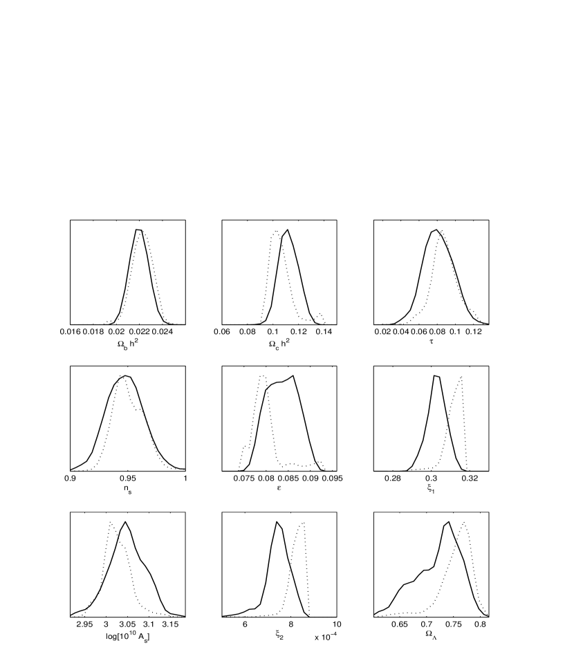
Figure 2: One dimensional marginalized posterior probability distribution (solid lines) and mean likelihood (dotted lines) for the cosmological parameters.

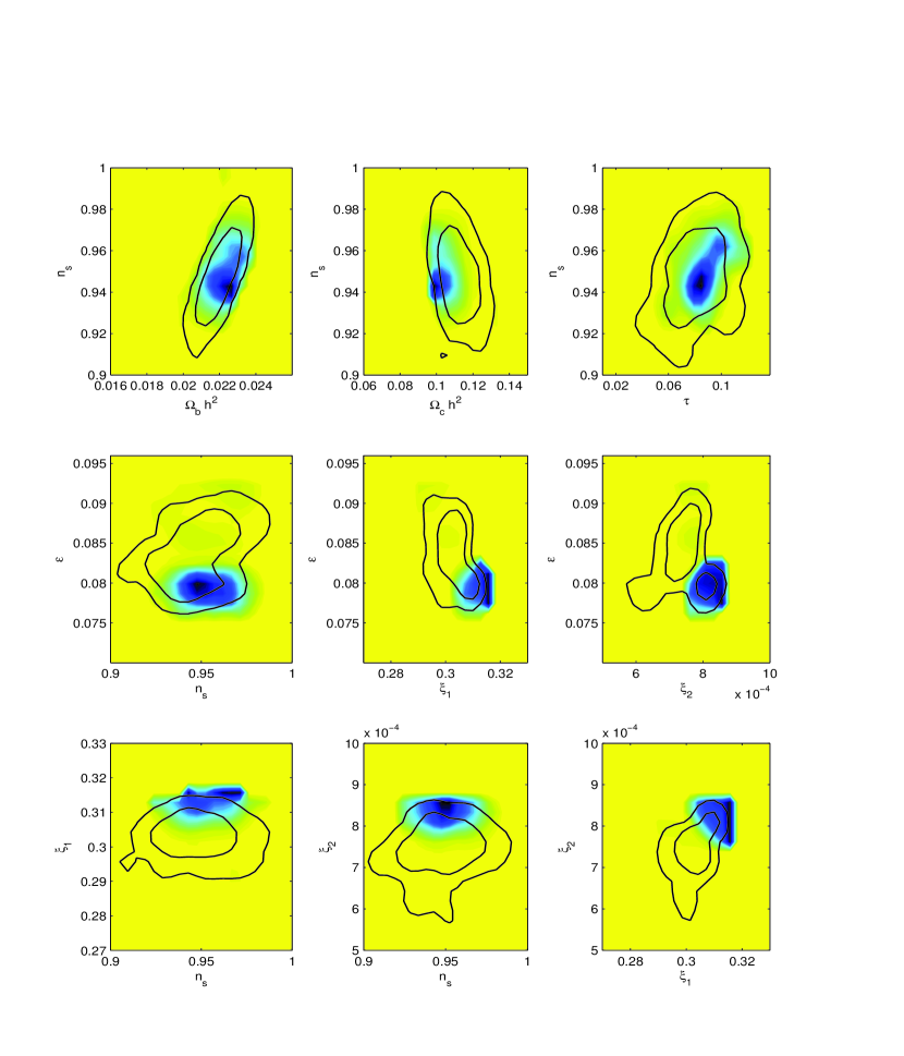
Figure 3: Posterior constraint for our model. The contours show the 68 % and 95 % confidence limits from the marginalized distribution.

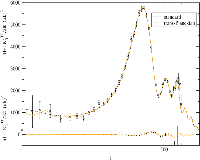
Figure 4: The best fit obtained for our trans-Planckian angular TT (up) and TE (down) power spectrum compared to the best fit standard inflationary power spectrum and five years WMAP data.

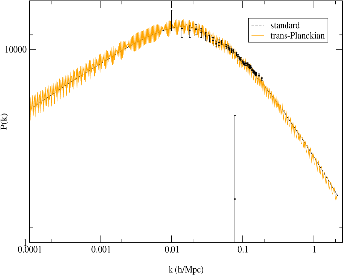
Figure 5: Predicted matter power spectrum for our trans-Planckian model compared to the 2dF data[70].

Table 1 shows the best fit parameters found by CosmoMC for the case $\xi_{1}=0$ (standard inflationary model) and $\xi_{1}\neq 0$ (trans-Planckian model). For the case of $\xi_{1}=0$ the standard values for the cosmological parameters [62] are recovered. We can estimate the scale of noncommutativity, $\frac{1}{\sqrt{\theta}}=\Lambda_{NC}$, from the trans-Planckian parameter $\xi_{2}=H/\Lambda_{NC}\approx 10^{-4}$. If the scale of $H$ during inflation is approximated to be of the order of $H\geq 10^{12}$ GeV [63], then the noncommutative scale is estimated as $\Lambda_{NC}\geq 10^{16}$ GeV. On the other hand as Refs. [64, 65, 66, 67] have demonstrated, the Minimal Supersymmetric Standard Model (MSSM) has all the ingredients to give rise to successful inflation. The MSSM inflation occurs at low scales i.e. $H\geq 1$ GeV. Then this put a bound on the scale of noncommutativity as $\Lambda_{NC}\geq 10^{4}$ GeV. Similar bounds on noncommutative scale, has reported in [68] using the investigation of Lorentz symmetry violation due to noncommutativity during experiments and also in [69] by studying of hydrogen atom spectrum and the Lamb-shift effect on a noncommutative space which is $\Lambda_{NC}\geq 10$ TeV.

6 Conclusion

We showed that a modification in the action of one inflaton due to noncommutativity, leads to a nonzero Bogoliubov coefficient $\beta_{k}$ which affects the power spectrum to have oscillatory corrections. Using CosmoMC code we showed that these corrections cause a drop in the WMAP $\chi^{2}$ of about $\Delta\chi^{2}\sim 8.5$. We also derived the noncommutative scale using parameters estimated by CosmoMC. Tacking the scale of inflation to be $H\geq 10^{12}$ GeV, we can estimate the scale of noncommutativity which yields $\Lambda_{NC}\geq 10^{16}$ GeV and with the scale of inflation $H\geq 1$ GeV, we get $\Lambda_{NC}\geq 10^{4}$ GeV.

References

- [1] J. Martin and R. H. Brandenberger, The Trans-Planckian problem of inflationary cosmology, Phys. Rev. D63 (2001) 123501, [hep-th/0005209].
- [2] J. Martin and R. H. Brandenberger, A cosmological window on trans-Planckian physics , [astro-ph/0012031].
- [3] S. Tsujikawa, R. Maartens and R. Brandenberger, Non-commutative inflation and the CMB , Phys. Lett. B574 (2003) 141, [astro-ph/0308169].
- [4] R. Easther, B. R. Greene, W. H. Kinney and G. Shiu, Imprints of short distance physics on inflationary cosmology , Phys. Rev. D67 (2003) 063508, [hep-th/0110226]; S. Shankaranarayanan, Is there an imprint of Planck scale physics on inflationary cosmology?, Class. Quant. Grav. 20 (2003) 75, [gr-qc/0203060]; A. Ashoorioon, J. L. Hovdebo and R. B. Mann, Running of the spectral index and violation of the consistency relation between tensor and scalar spectra from trans-Planckian physics, Nucl. Phys. B 727, 63 (2005), [arXiv:gr-qc/0504135].
- [5] R. Easther, B. R. Greene, W. H. Kinney and G. Shiu, A generic estimate of trans-Planckian modifications to the primordial power spectrum in inflation , Phys. Rev. D66 (2002) 023518, [hep-th/0204129].
- [6] B. Greene, M. Parikh and J. P. van der Schaar, Universal correction to the inflationary vacuum, JHEP 0604 (2006) 057, [hep-th/0512243].
- [7] T. Tanaka, A comment on trans-Planckian physics in inflationary universe , [astro-ph/0012431].
- [8] J. C. Niemeyer and R. Parentani, Trans-Planckian dispersion and scale-invariance of inflationary perturbations , Phys. Rev. D64 (2001) 101301, [astro-ph/0101451].
- [9] A. Kempf and J. C. Niemeyer, Perturbation spectrum in inflation with cutoff , Phys. Rev. D64 (2001) 103501, [astro-ph/0103225].
- [10] D. Campo, J. Niemeyer and R. Parentani, Damped corrections to inflationary spectra from a fluctuating cutoff , arXiv:0705.0747v1 [hep-th].
- [11] A. A. Starobinsky, Robustness of the inflationary perturbation spectrum to trans-Planckian physics , Pisma Zh. Eksp. Teor. Fiz. 73 (2001) 415; JETP Lett. 73 (2001) 371, [astro-ph/0104043].
- [12] U. H. Danielsson, A note on inflation and transplanckian physics , Phys. Rev. D66 (2002) 023511, [hep-th/0203198].
- [13] K. Goldstein and D. A. Lowe, Initial state effects on the cosmic microwave background and trans-planckian physics , Phys. Rev. D67 (2003) 063502, [hep-th/0208167].
- [14] C. P. Burgess, J. M. Cline, F. Lemieux and R. Holman, Are inflationary predictions sensitive to very high energy physics?, JHEP 0302 (2003) 048, [hep-th/0210233].
- [15] J. Macher and R. Parentani, Signatures of trans-Planckian dispersion in inflationary spectra, arXiv:0804.1920v3 [hep-th].
- [16] P. R. Anderson, C. Molina-Paris and E. Mottola, Short distance and initial state effects in inflation: stress tensor and decoherence , Phys. Rev. D72 (2005) 043515, [hep-th/0504134].
- [17] C. Armendariz-Picon and E. A. Lim, Vacuum choices and the predictions of inflation , JCAP 0312 (2003) 006, [hep-th/0303103].
- [18] H. Collins and R. Holman, Trans-planckian signals from the breaking of local Lorentz invariance , arXiv: 0705.4666v1 [hep-ph].
- [19] A. R. Liddle and D. H. Lyth, Cosmological inflation and large-scale structure, Cambridge University Press (2000).
- [20] V. Mukhanov, Physical foundations of cosmology, Cambridge University Press (2005).
- [21] C. P. Burgess, Lectures on cosmic inflation and its potential stringy realizations , arXiv: 0708.2865v1 [hep-th].
- [22] A. Linde, Inflationary cosmology, arXiv: 0705.0164v2 [hep-th].
- [23] J. Garcia-Bellido, Cosmology and astrophysics , [astro-ph/0502139].
- [24] J. Niemeyer, R. Parentani and D. Campo, Minimal modifications of the primordial power spectrum from an adiabatic short distance cutoff , arXiv: 0705.0747v1 [hep-th].
- [25] J. Martin and R. H. Brandenberger, On the dependence of the spectra of fluctuations in inflationary cosmology on trans-Planckian physics , Phys. Rev. D68 (2003) 063513, [hep-th/0305161].
- [26] N. Kaloper, M. Kleban, A. E. Lawrence and S. Shenker, Signatures of short distance physics in the Cosmic Microwave Background Phys. Rev. D 66, 123510 (2002) [hep-th/0201158].
- [27] R. H. Brandenberger and J. Martin, Back-Reaction and the Trans-Planckian problem of inflation revisited , Phys. Rev. D71 (2005) 023504, [hep-th/0410223]; M. Lemoine, M. Lubo, J. Martin and J. P. Uzan, The stress-energy tensor for trans-Planckian cosmology, Phys. Rev. D 65 (2002) 023510, [arXiv:hep-th/0109128].
- [28] R. H. Brandenberger and J. Martin, On Signatures of short distance physics in the Cosmic Microwave Background , Int. J. Mod. Phys. A17 (2002) 3663, [hep-th/0202142].
- [29] S. Weinberg, Effective field theory for inflation, arXiv:0804.4291v2 [hep-th].
- [30] J. Martin and C. Ringeval, superimposed oscillations in the WMAP data?, Phys. Rev. D69 (2004) 083515, [astro-ph/0310382].
- [31] J. Martin and C. Ringeval, Addendum to ”Superimposed oscillations in the WMAP data?” , Phys. Rev. D69 (2004) 127303, [astro-ph/0402609].
- [32] J. Martin and C. Ringeval, Exploring the Superimposed Oscillations Parameter Space, JCAP 0501 (2005) 007, [hep-ph/0405249].
- [33] N. E. Groeneboom and O. Elgaroy, Detection of transplanckian effects in the cosmic microwave background, Phys. Rev. D 77, 043522 (2008), arXiv: 0711.1793v4 [astro-ph]
- [34] N. D. Birrell and P. C. W. Davies, Quantum fields in curved space, Cambridge University Press, 1982.
- [35] T. S. Bunch and P. C. Davies, Proc. Roy. Soc. Lond. A360 (1978) 117.
- [36] K. Schalm, G. Shiu, J. P. van der Schaar, The cosmological vacuum ambiguity, effective actions, and transplanckian effects in inflation, [hep-th/0412288].
- [37] I. S. Gradshteyn and I. M. Ryzhik, Table of Integrals, Series, and Products , Fifth edition, Academic Press Inc., London, (1994).
- [38] L. Sriramkumar and T. Padmanabhan, Initial state of matter fields and trans-Planckian physics: Can CMB observations disentangle the two? Phys. Rev. D71 (2005) 103512, [gr-qc/0408034].
- [39] Yi-Fu Cai, Tao-tao Qiu, Jun-Qing Xia, Xinmin Zhang, A Model Of Inflationary Cosmology Without Singularity, arXiv:0808.0819 [astro-ph].
- [40] Yi-fu Cai and Yun-Song Piao, Probing noncommutativity with inflationary gravitational waves, Phys. Lett. B657 (2007) 1, [gr-qc/0701114].
- [41] M. R. douglas and N. A. Nekrasov, Noncommutative field theory, Rev. Mod. Phys. 73 (2001) 977, [hep-th/0106048].
- [42] R. J. Szabo, Quantum field theory on noncommutative space, Phys. Rept. 378 (2003) 207, [hep-th/0109162].
- [43] M. R. douglas and N. A. Nekrasov, Noncommutative field theory, Rev. Mod. Phys. 73 (2001) 977, [hep-th/0106048].
- [44] R. J. Szabo, Quantum field theory on noncommutative space, Phys. Rept. 378 (2003) 207, [hep-th/0109162].
- [45] S. Minwalla, M. V. Raamsdonk and N. Seiberg, Noncommutative perturbative dynamics, JHEP 02 (2000) 020, [hep-th/9912072].
- [46] H. Grosse and R. Wulkenhaar, Renormalisation of -theory on noncommutative in the matrix base , Commun. Math. Phys. 256 (2005) 305, [hep-th/0401128].
- [47] R. Gurau, J. Magnen, V. Rivasseau and A. Tanasa, A translation-invariant renormalizable non-commutative scalar model , arXiv: 0802.0791v1 [math-ph].
- [48] B. Mirza, M. Zarei, Effective field theory of a locally noncommutative space-time and extra dimensions , arXiv: 0803.0232v1 [hep-th].
- [49] E. Langmann, R. J. Szabo, Duality in Scalar Field Theory on Noncommutative Phase Spaces, Phys. Lett. B533 (2001) 168, [hep-th/0202039].
- [50] A. Lewis and S. Bridle, Phys. Rev. D66, 103511 (2002), [astro-ph/0205436], http://cosmologist.info/cosmomc.
- [51] L. Bergstrom and U .H. Danielsson, Can MAP and Planck map Planck physics?, JHEP 0212 (2002) 038, [hep-th/0211006].
- [52] W. Hu and S. Dodelson, Cosmic Microwave Background Anisotropies, Ann. Rev. Astron. Astrophys. 40 (2002) 171, [astro-ph/0110414].
- [53] J. M. Cline, P. Crotty and J. Lesgourgues, Does the small CMB quadrupole moment suggest new physics? , JCAP 0309 (2003) 010, [astro-ph/0304558].
- [54] S. Hannestad and L. Mersini-Houghton, A first glimpse of string theory in the sky? , Phys. Rev. D71 (2005) 123504, [hep-ph/0405218].
- [55] C. R. Contaldi, M. Peloso, L. Kofman and A. Linde, Suppressing the lower Multipoles in the CMB Anisotropies , JCAP 0307 (2003) 002, [astro-ph/0303636].
- [56] R. Easther, W. H. Kinney and H. Peiris, Boundary Effective Field Theory and Trans-Planckian Perturbations: Astrophysical Implications, JCAP 0508 (2005) 001, [astro-ph/0505426].
- [57] N. E. Groeneboom and O. Elgaroy, Detection of transplanckian effects in the cosmic microwave background, Phys. Rev. D77 043522 (2008), arXiv:0711.1793v4 [astro-ph].
- [58] O. Elgaroy and S. Hannestad, Can Planck-scale physics be seen in the cosmic microwave background ?, Phys.Rev. D68 (2003) 123513, [astro-ph/0307011].
- [59] J. Hamann, S. Hannestad, M. S. Sloth and Y. Y. Y. Wong, Observing trans-Planckian ripples in the primordial power spectrum with future large scale structure probes, arXiv: 0807.4528v1 [astro-ph].
- [60] A. Lewis, A. Challinor and A. Lasenby, Astrophys. J. 538, 473 (2000), [astro-ph/9911177], http://camb.info.
- [61] http://lambda.gsfc.nasa.gov
- [62] E. Komatsu et al., Five-Year Wilkinson Microwave Anisotropy Probe (WMAP) Observations: Cosmological Interpretation, arXiv:0803.0547 [astro-ph].
- [63] N. Bartolo, E. Komatsu, S. Matarrese and A. Riotto, Non-Gaussianity from Inflation: Theory and Observations, Phys. Rept. 402 (2004) 103, [astro-ph/0406398].
- [64] R. Allahverdi, J. Garcia-Bellido, K. Enqvist and A. Mazumdar, Gauge invariant MSSM inflaton, Phys. Rev. Lett. 97 (2006) 191304, [hep-ph/0605035].
- [65] R. Allahverdi, A. Kusenko and A. Mazumdar, A-term inflation and the smallness of the neutrino masses, [hep-ph/0608138].
- [66] R. Allahverdi, K. Enqvist, J. Garcia-Bellido, A. Jokinen and A. Mazumdar, MSSM flat direction inflation: slow roll, stability, fine tunning and reheating, [hep-ph/0610134].
- [67] R. Allahverdi, B. Dutta and A. Mazumdar, Unifying inflation and dark matter with neutrino masses , arXiv: 0708.3983 [hep-ph].
- [68] S. M. Carroll, J. A. Harvey, V. A. Kostelecky, C. D. Lane, T. Okamoto, Noncommutative Field Theory and Lorentz Violation, Phys. Rev. Lett. 87 (2001) 141601, [hep-th/0105082].
- [69] M. Chaichian, M. M. Sheikh-Jabbari, A. Tureanu, Hydrogen atom spectrum and the Lamb shift in noncommutative QED, Phys. Rev. Lett. 86 (2001) 2716, [hep-th/0010175].
- [70] S. Cole and et al., The 2dF Galaxy Redshift Survey: Power-spectrum analysis of the final dataset and cosmological implications Mon. Not. Roy. Astron. Soc. 362 (2005) 505, [astro-ph/0501174].