Pinning down the Invisible Sneutrino

Abstract:

For points in SUSY parameter space where the sneutrino is lighter than the lightest chargino and next-to-lightest neutralino, its direct mass determination from sneutrino pair production process at $e^{+}e^{-}$ collider is impossible since it decays invisibly. In such a scenario the sneutrino can be discovered and its mass determined from measurements of two-body decays of charginos produced in pairs at the ILC. Using the event generator WHIZARD we study the prospects of measuring sneutrino properties in a realistic ILC environment. In our analysis we include beamstrahlung, initial state radiation, a complete account of reducible backgrounds from SM and SUSY processes, and a complete matrix-element calculation of the SUSY signal which encompasses all irreducible background and interference contributions. We also simulate photon induced background processes using exact matrix elements. Radiation effects and the cuts to reduce background strongly modify the edges of the lepton energy spectra from which the sneutrino and chargino mass are determined. We discuss possible approaches to measure the sneutrino mass with optimal precision.

1 Introduction

Supersymmetry (SUSY) [1] is one of the best-motivated extensions of the Standard Model (SM): it stabilizes the hierarchy between the electroweak (EW) scale and the Planck scale and naturally explains EW symmetry breaking by a radiative mechanism. The naturalness of the scale of electroweak symmetry breaking and the Higgs mass places a rough upper bound on the superpartner masses of several TeV. This gives the Large Hadron Collider (LHC) the opportunity to discover the superpartners within the next years [2]. Due to the LHC’s hadronic environment, mostly strongly interacting sparticles will be produced with light sleptons and weakly interacting gauginos appearing in decay cascades of squarks and gluinos. Heavy weakly interacting states will be especially hard to detect at the LHC and their high-precision spectroscopy will only be possible at a future high-energy International Linear Collider (ILC) [3].

In this paper we focus on scenarios within the Minimal Supersymmetric Standard Model (MSSM), in which sneutrinos are lighter than the lightest chargino and next-to-lightest neutralino. Sneutrino decays to charged particles in the final state are then of higher order and therefore strongly suppressed (e.g. a 4-body decay is suppressed by an off-shell intermediate propagator and two additional powers of the weak coupling constant). As a result, sneutrinos decay completely invisibly into a neutrino and the lightest supersymmetric particle (LSP, the lightest neutralino in the considered case). A sneutrino appearing in a cascade at the LHC is hence lost and cannot be reconstructed. An ILC threshold scan is precluded for the very same reason. The only possibility to access the sneutrino mass in such a case is to select a well-reconstructible process where the sneutrino is exchanged in a $t$-channel or shows up as a part of a cascade decay. The precise determination of kinematic distributions gives then access to the sneutrino mass. This idea has been proposed in Ref. [4], where it was argued that background effects are sufficiently under control, so a precise mass determination is possible.

Here we study the prospects for determining sneutrino properties in a realistic ILC environment. We include beamstrahlung, initial-state radiation, a complete account of reducible backgrounds from SM and SUSY processes, and a complete matrix-element calculation of the SUSY signal which encompasses all irreducible background and interference contributions. Radiation, background and interference do have considerable effect on spectrum shapes and edges, and we discuss the possible approaches to nevertheless determine the sneutrino mass with optimal precision. An interesting question is how well this can be done in a scenario with nearly degenerate charginos and sleptons, where the corresponding decay leptons are fairly soft and are in danger of being swamped by photon-induced background. We restrict ourselves to areas in SUSY parameter space where charginos are within reach of a 500 GeV ILC.

As a working point we take the SPS1a’ scenario [6] which has been widely in use for phenomenological studies. It is derived from the SPS1a point [7] by lowering the universal scalar mass parameter in order to satisfy the cold dark matter constraint. Such a shift leads to lower sfermion masses and, as a result, predicts sneutrinos that decay invisibly. The SPS1a’ satisfies all experimental constraints from precision data and cosmology.

The paper is organized as follows. In Sec. 2 we discuss in detail the signal and background processes, especially investigating whether they are experimentally distinguishable or not. Effects coming from the inclusion of initial state radiation (ISR) as well as beamstrahlung are discussed. The cut-based strategy to enhance the signal-to-background ratio is developed in Sec. 3, where we discuss the influence of the cut procedure on the quality of the measurement of several observables. The crucial observation here is the distortion of the lepton energy spectra due to ISR and photon-induced processes as decay leptons are quite soft in almost degenerate scenarios like SPS1a’. All analyses in this Section have been done for a $500$ GeV center-of-mass (CM) energy apart from Sec. 3.3, where important differences for an 800 GeV ILC are discussed. In Sec. 4, we present different approaches to the sneutrino mass determination in our framework. Finally, we conclude as well as give an outlook.

For reader’s convenience, Appendix A recapitulates masses and branching ratios (BRs) of supersymmetric particles for the SPS1a’ parameter point that are important for our analysis. Appendix B is devoted to the comparison of the effective photon approximation (EPA) with the exact matrix element method employed in our calculations.

2 Signal and background processes

After SUSY will have been found and identified at the LHC, the goal of the ILC will be the precision determination of the masses, quantum numbers and coupling constants in order to get access to the high-energy theory and possibly the SUSY breaking mechanism [6]. Especially challenging are measurements of sneutrino parameters in scenarios in which they decay invisibly, as in e.g. the SPS1a’ parameter point. The difficulty lies not only in an inability of exploiting the sneutrino pair production process, but also in particularly many background processes, both of SUSY and SM origin, contributing to the signal signature as discussed below.

2.1 Sneutrino signal and signature

One of the standard candle processes is the pair production of the lightest chargino,

$$e^{+}e^{-}\,\rightarrow\,\widetilde{\chi}^{+}_{1}\widetilde{\chi}^{-}_{1}\,\,.$$ (1)

The chargino mass can be measured either by a threshold scan or in the continuum from the edges of the decay spectra [4]. In the SPS1a’ scenario the light charginos $\widetilde{\chi}^{+}_{1}$ decay predominantly to $\widetilde{\tau}^{+}_{1}\nu_{\tau}$ with a branching ratio BR($\widetilde{\chi}^{+}_{1}\to\widetilde{\tau}^{+}_{1}\nu_{\tau}$)=53.6% (see Table A.1 in Appendix A), followed by $\widetilde{\tau}^{+}_{1}\to\tau^{+}\widetilde{\chi}^{0}_{1}$. This cascade produces a final state similar to that of stau pair production. Using two tau jets in the opposite hemispheres and missing energy as the signature for $\widetilde{\chi}^{\pm}_{1}\widetilde{\chi}^{\mp}_{1}$ production, the measurement of the chargino mass has been simulated for the SPS1a scenario, and the expected accuracy is $0.55$ GeV [8, 9]. Detailed simulations showed that also the stau mass in SPS1a can be measured with an uncertainty of $0.30$ GeV [10, 11]. A similar precision for the SPS1a’ point can be expected, since – in addition – chargino decays to electron (or muon) and sneutrino can be exploited.

The main objective of our work, however, is to measure the sneutrino mass, where we assume the first and second generation sneutrinos ($\widetilde{\nu}_{e}$ and $\widetilde{\nu}_{\mu}$) to be mass degenerate. This can be done by investigating the chargino decay modes $\widetilde{\chi}^{+}_{1}\to\widetilde{\nu}_{\ell}\ell^{+}$, $\ell=e,\mu$, in chargino pair production process [4]. With a BR($\widetilde{\chi}^{+}_{1}\to\widetilde{\nu}_{\ell}\ell^{+}$)=13% a large sample of events can be expected in this channel. The two-body chargino decay leads to a uniform decay lepton energy spectrum with edges determined by the chargino and sneutrino masses, which provides a method for their experimental determination.

In order to avoid large backgrounds from same-flavor lepton and slepton production, it is advantageous to select events with leptons of different flavor, i.e. one of the charginos decays to an electron, the other to a muon. So, we search for (semi-)exclusive final states:

$$e^{+}e^{-}\,\rightarrow\,\widetilde{\chi}^{+}_{1}\widetilde{\chi}^{-}_{1}\,\rightarrow\,\widetilde{\nu}_{e}^{*}e^{-}\widetilde{\nu}_{\mu}\mu^{+}\,\rightarrow\,e^{-}\,\mu^{+}\,\bar{\nu}_{e}\,\nu_{\mu}\,\widetilde{\chi}^{0}_{1}\,\widetilde{\chi}^{0}_{1}\,.$$ (2)

There are also other channels that contribute to the (semi-)exclusive final state as in Eq. (2),

$$e^{+}e^{-}\,\rightarrow\,X\rightarrow\,e^{-}\,\mu^{+}\,\bar{\nu}_{e}\,\nu_{\mu}\,\widetilde{\chi}^{0}_{1}\,\widetilde{\chi}^{0}_{1}\,,$$ (3)

with the intermediate state $X$ that includes different production processes as well as interference terms, e.g. multi-peripheral diagrams, chargino decays into neutralino and $W$, smuon $\widetilde{\mu}^{+}_{i}\widetilde{\mu}_{j}^{-}$ and selectron $\widetilde{e}^{+}_{i}\widetilde{e}_{j}^{-}$ pair production, and single-resonant SM di-boson production. In the following, we will distinguish between the “proper” signal, where the final state products come from chargino pairs decaying to electron and muon sneutrinos as in Eq. (2), and the signal including irreducible background, Eq. (3). If not mentioned otherwise, numbers and cross sections labeled “signal” always include these irreducible background processes. The mixed chargino decay modes, where one chargino decays as $\widetilde{\chi}^{+}_{1}\to\widetilde{\nu}_{\ell}\ell^{+}$ and the other $\widetilde{\chi}^{-}_{1}\to\widetilde{\tau}^{-}_{1}\bar{\nu}_{\tau}$ followed by the cascade of $\widetilde{\tau}$ and leptonic $\tau$ decays, will have additional neutrinos in the final state. Such processes are considered as reducible background. All reducible SUSY backgrounds that contain additional neutrinos in the final state will be treated in Sec. 2.2.

At the ILC, for the SUSY spectrum of SPS1a’, the Born cross section for $\widetilde{\chi}_{1}^{\pm}$ pair production without initial-state radiation or beamstrahlung is $173.56$ fb at a CM energy of 500 GeV. The cross section reaches its maximum of $\sim$200 fb near $\sqrt{s}=600$ GeV, and then decreases to $181.30$ fb at 800 GeV, and falls further to $141$ fb at 1 TeV, see Fig. 1 (tree level result shown together with the 1-loop corrections calculated in [5, 12, 13]). The chargino partial width for the decay into sneutrino and lepton is 10.2 MeV for each of the first two generations, which constitutes 13.3% of the total decay width each; branching fractions for other decay modes are 18.5% for tau sneutrino and tau, and the dominant decay with 53.6% is into stau and tau-neutrino. At 500 GeV the cross section for the proper signal $\sigma(e^{+}e^{-}\,\rightarrow\,\widetilde{\chi}^{+}_{1}\widetilde{\chi}^{-}_{1})\times BR(\widetilde{\chi}^{-}_{1}\,\rightarrow\,\widetilde{\nu}_{e}^{*}e^{-})\times BR(\widetilde{\chi}^{+}_{1}\,\rightarrow\,\widetilde{\nu}_{\mu}\mu^{+})$ is $3.06$ fb, whereas for the six-fermion final state, Eq. (3), it is 4.69 fb. This shows that there are considerable off-shell and interference effects from other non-resonant SUSY processes contributing to the same six-fermion final state (cf. also [14]). These effects are additionally smeared when ISR and beamstrahlung are taken into account; we then obtain 2.50 fb for the proper signal (i.e. when forcing the final state to come from chargino pairs decaying to sneutrinos) and 3.94 fb for the signal. As expected, both values are slightly lower when ISR and beamstrahlung are taken into account, as the emitted photons drive the process to slightly lower values of the effective CM energy and hence lower chargino cross section. For a CM energy of 800 GeV, the respective numbers including initial state radiation and beamstrahlung are 6.60 fb for the signal and 3.23 fb for the proper signal. Here, the discrepancy between full matrix elements and narrow-width approximation is even more severe since more SUSY processes can contribute to the exclusive final state.

Figure 1: Total cross section for chargino pair production for the point SPS1a’, at LO (medium grey, red). The NLO curves show a fixed order approach (black, blue) and with photon resummation (light grey, green) (from [5, 12]).

Experimentally, the signature for the signal process is one electron and one anti-muon and missing energy,

$$e^{+}e^{-}\,\rightarrow\,e^{-}\mu^{+}\,+\,\mathchoice{\ooalign{$\hfil\displaystyle\mkern 0.0mu/\hfil$\crcr$\displaystyle E$}}{\ooalign{$\hfil\textstyle\mkern 0.0mu/\hfil$\crcr$\textstyle E$}}{\ooalign{$\hfil\scriptstyle\mkern 0.0mu/\hfil$\crcr$\scriptstyle E$}}{\ooalign{$\hfil\scriptscriptstyle\mkern 0.0mu/\hfil$\crcr$\scriptscriptstyle E$}}\;.$$ (4)

Such final states with two visible leptons and missing energy, however, are generated by many other processes, both with supersymmetric and Standard Model particles in the intermediate states. Many of these processes should be suppressed both by phase space and higher orders in the electroweak coupling constant. On the other hand, photon-induced processes – enhanced by large collinear logarithms – give by their sheer cross sections the most severe background at the ILC. In the following, we will classify the reducible and irreducible background processes from SM as well as SUSY productions.

2.2 Reducible SUSY background

Contamination from other SUSY processes comes from any process with the generic signature

$$e^{+}e^{-}\rightarrow\mbox{any SUSY particles}\,\rightarrow\,\widetilde{\chi}^{0}_{1}\,\widetilde{\chi}^{0}_{1}\,e^{-}\,\mu^{+}\,+n\nu\;,$$ (5)

with $n\geq 4$. Especially severe contaminations come from processes that lead to two leptonically decaying $\tau$’s. They mainly originate from the production of mixed neutralino pairs $\widetilde{\chi}^{0}_{i}\widetilde{\chi}^{0}_{j}$, stau pairs as well as chargino pairs. The latter then undergo the subsequent decays to stau and LSP or tau and sneutrino.

In listing the contributing processes, there is a tension between describing them signature-driven or considering them according to their exclusive production mechanisms. Since there are big off-shell and interference effects among several contributing weak amplitudes, as was shown above from the cross section considerations, it is difficult and dangerous to split processes completely into their corresponding production channels. (Also at the ILC, SUSY processes appear to have a generic cascade chain structure, but due to their production being electroweak, a lot more interference among different chains is possible and actually sizable). On the other hand, an experimental description which takes into account only visible particles and missing energy is not much discriminating. We here pursue the convention to classify processes as SUSY or SM according to whether they come from SUSY or SM production, which is apparent from the LSP’s in the final state.

Process	500 GeV	$\sigma$ [fb], presel.	$\sigma^{\text{cut}}$ [fb]
Signal	$ee\to e\mu\bar{\nu}_{e}\nu_{\mu}\tilde{\chi}_{1}^{0}\tilde{\chi}_{1}^{0}$	$3.940(\phantom{3}8)$	$1.639(3)$
SUSY $\tau$ Bkgd.	$ee\to\tau\tau\tilde{\chi}_{1}^{0}\tilde{\chi}_{1}^{0}\to e\mu\tilde{\chi}_{1}^{0}\tilde{\chi}_{1}^{0}4\nu$	$4.107(\phantom{3}7)$	$0.978(2)$
SUSY $\tau\nu$ Bkgd.	$ee\to\tau\tau\tilde{\chi}_{1}^{0}\tilde{\chi}_{1}^{0}2\nu\to e\mu\tilde{\chi}_{1}^{0}\tilde{\chi}_{1}^{0}6\nu$	$3.245(10)$	$0.818(3)$
SUSY $\tau e$ Bkgd.	$ee\to e\tau\bar{\nu}_{e}\nu_{\tau}\tilde{\chi}_{1}^{0}\tilde{\chi}_{1}^{0}\to e\mu\tilde{\chi}_{1}^{0}\tilde{\chi}_{1}^{0}4\nu$	$3.691(\phantom{3}9)$	$1.102(8)$
SUSY $\tau\mu$ Bkgd.	$ee\to\mu\tau\nu_{\mu}\bar{\nu}_{\tau}\tilde{\chi}_{1}^{0}\tilde{\chi}_{1}^{0}\to e\mu\tilde{\chi}_{1}^{0}\tilde{\chi}_{1}^{0}4\nu$	$2.617(10)$	$0.966(8)$
SM $WW$ Bkgd.	$ee\to e\mu 2\nu$	$152.42(25)\phantom{3}$	$0.736(2)$
SM $e\tau$ Bkgd.	$ee\to e\tau 2\nu\to e\mu 4\nu$	$26.522(12)$	$0.317(1)$
SM $\mu\tau$ Bkgd.	$ee\to\mu\tau 2\nu\to e\mu 4\nu$	$15.569(54)$	$0.174(1)$
SM $\nu$ Bkgd.	$ee\to e\mu 4\nu$	$0.145(\phantom{3}1)$	$0.016(3)$
SM $\tau$ Bkgd.	$ee\to\tau\tau\to e\mu 4\nu$	$32.679(98)$	$<0.001$
SM $\tau\nu$ Bkgd.	$ee\to\tau\tau 2\nu\to e\mu 6\nu$	$3.852(10)$	$0.335(9)$
SM $\gamma\to\tau$ Bkgd.	$\gamma^{*}\gamma^{*}\to\tau\tau\to e\mu 2\nu$	$21392(70)\phantom{3}\phantom{3}\phantom{3}$	$0.273(2)$
SM $\gamma\to c$ Bkgd.	$\gamma^{*}\gamma^{*}\to c\bar{c}\to e\mu jj2\nu$	$1089(\phantom{3}4)\phantom{3}\phantom{3}\phantom{3}$	$<0.001$
SM $\gamma\to W$ Bkgd.	$\gamma^{*}\gamma^{*}\to WW\to e\mu 2\nu$	$1.094(\phantom{3}6)$	$0.079(1)$
SM $\gamma\to\tau\nu_{\tau}$ Bkgd.	$\gamma^{*}\gamma^{*}\to\tau\tau 2\nu\to e\mu 8\nu$	$0.077(\phantom{3}1)$	$<0.001$
SM $\gamma\to\ell\tau$ Bkgd.	$\gamma^{*}\gamma^{*}\to(e,\mu)\tau 2\nu\to e\mu 4\nu$	$0.404(\phantom{3}2)$	$0.055(2)$

Table 1: Cross sections for all signal and background processes for an ILC energy of 500 GeV. ISR and beamstrahlung are always included. Note that the final states $e$ always means electron and $\mu$ always anti-muon. For more details about the processes confer the text. The “presel.” column always includes a $5^{\circ}$ cut for the final electron to cut out collinear regions, and for the $\gamma$-induced processes a $1^{\circ}$ cut for particles vanishing in the beampipe. The last column shows cross sections after the cuts discussed in Sec. 3. In parentheses are the WHIZARD integration errors.

In the following we classify signal and background according to the production mechanism if it is clearly identifiable (especially for the SM processes), or specifically for the SUSY processes we use the SM particles that appear together with the LSP in the final state (before a final leptonic $\tau$ decay).

In our analyses we consider as (reducible) SUSY background all processes that produce final states with $e^{-}\mu^{+}$, two lightest neutralinos (LSP) and four or six neutrinos. For the parameter point SPS1a’, the sum of these SUSY processes gives event numbers for the signal signature that are bigger than the signal typically by a factor three to four.

We distinguish the following SUSY background processes in our study, according to the number of intermediate state $\tau$’s and $\nu_{\tau}$’s, because $\tau$ decays are technically treated differently (see below, Sec. 2.4). Furthermore, the $\tau$’s are considerably long-lived such that there is no interference with non-resonant diagrams, and the processes can be well split here. The largest contribution comes from two LSP’s together with a tau pair, giving rise to the two tagged leptons $e\mu$, four neutrinos and two LSP’s: $e^{+}e^{-}\to X\to\tau^{+}\tau^{-}\widetilde{\chi}^{0}_{1}\widetilde{\chi}^{0}_{1}\to\widetilde{\chi}^{0}_{1}\,\widetilde{\chi}^{0}_{1}e^{-}\mu^{+}\nu_{\mu}\bar{\nu}_{e}\nu_{\tau}\bar{\nu}_{\tau}$. The main contribution to this final state – which we call SUSY $\tau$ background – comes from on-shell stau pair production $\widetilde{\tau}^{+}_{i}\widetilde{\tau}^{-}_{j}$, as well as from neutralino pair $\widetilde{\chi}^{0}_{1}\widetilde{\chi}^{0}_{2}$ production in the intermediate state $X$. This process receives also smaller contributions from other intermediate $X$: neutralino pairs $\widetilde{\chi}^{0}_{i}\widetilde{\chi}^{0}_{j}$ (especially $\widetilde{\chi}^{0}_{1}\widetilde{\chi}^{0}_{3}$), production of heavy chargino $\widetilde{\chi}^{+}_{1}\widetilde{\chi}^{-}_{2}$ (on-shell only at 800 GeV), and even Higgstrahlung or SM di-boson production with (partial) decay into SUSY particles.

Since we are exclusively looking into positively charged muons and negatively charged electrons, there are processes with two different intermediate states containing a single $\tau$: $e^{+}e^{-}\to X\to\mu^{+}\nu_{\mu}\tau^{-}\bar{\nu}_{\tau}\widetilde{\chi}^{0}_{1}\widetilde{\chi}^{0}_{1}\to\widetilde{\chi}^{0}_{1}\,\widetilde{\chi}^{0}_{1}e^{-}\mu^{+}\nu_{\mu}\bar{\nu}_{e}\nu_{\tau}\bar{\nu}_{\tau}$, and $e^{+}e^{-}\to X\to e^{-}\bar{\nu}_{e}\tau^{+}\nu_{\tau}\widetilde{\chi}^{0}_{1}\widetilde{\chi}^{0}_{1}\to\widetilde{\chi}^{0}_{1}\widetilde{\chi}^{0}_{1}e^{-}\mu^{+}\nu_{\mu}\bar{\nu}_{e}\nu_{\tau}\bar{\nu}_{\tau}$. For both of these processes, the main contributing intermediate states are chargino pairs $\widetilde{\chi}^{+}_{1}\widetilde{\chi}_{1}^{-}$ with one of the charginos decaying directly to electron or muon and the other decaying to $\tau$. The other possible double-resonant contributions are, for example, production of neutralino pairs $\widetilde{\chi}^{0}_{1}\widetilde{\chi}_{3,4}^{0}$, stau pairs $\widetilde{\tau}^{+}_{i}\widetilde{\tau}_{j}^{-}$, and smuon $\widetilde{\mu}^{+}_{i}\widetilde{\mu}_{j}^{-}$ or selectron pairs $\widetilde{e}^{+}_{i}\widetilde{e}_{j}^{-}$, respectively. Single-resonant contributions include SM $W$ pairs, production of heavy charginos $\widetilde{\chi}^{+}_{1}\widetilde{\chi}^{-}_{2}$, the supersymmetrized version of vector boson fusion processes (VBF) (e.g. replacing the VBF final state $e^{+}W^{-}\nu$ by $e^{+}\widetilde{\chi}^{-}_{i}\widetilde{\nu}$) and tri-boson production. Because of the electron in the final state of the second process, there are many more VBF processes and peripheral $t$-channel topologies.

The most complex process – the SUSY $\tau\nu$ background – is the one which contains in addition to the SUSY $\tau$ background also two neutrinos in the intermediate state: $e^{+}e^{-}\to X\to\tau^{+}\tau^{-}\nu_{i}\bar{\nu}_{i}\widetilde{\chi}^{0}_{1}\widetilde{\chi}^{0}_{1}\to\widetilde{\chi}^{0}_{1}\widetilde{\chi}^{0}_{1}e^{-}\mu^{+}\nu_{\mu}\bar{\nu}_{e}\nu_{\tau}\bar{\nu}_{\tau}\nu_{i}\bar{\nu}_{i}$, $i=e,\mu,\tau$, which yields 60,000 Feynman diagrams before the final $\tau$ decays. The leading contribution is again due to production of chargino pairs $\widetilde{\chi}^{+}_{1}\widetilde{\chi}^{-}_{1}$ and the following decays to $\tau$ leptons. The other possibility is production of neutralino pair $\widetilde{\chi}^{0}_{1}\widetilde{\chi}_{2}^{0}$ and processes similar to SUSY $\tau$ background with additional bremsstrahlung of electromagnetic and weak gauge bosons. By far the highest number of diagrams is for a heavy neutralino pair production with their subsequent decays (it becomes important at 800 GeV, where heavy neutralinos can be produced on-shell).

For the photon-induced SUSY processes, the largest contribution comes from stau pairs with a cross section of 0.028 fb at a 500 GeV ILC. Since it can be easily cut out, we do not consider any $\gamma$-induced SUSY background from now on.

2.3 Standard Model background processes

The SM backgrounds leading to the same signature of a different-flavor opposite-sign lepton pair and missing energy (carried away by neutrinos in the SM), mainly come from $WW$ pairs, single $W$ production and $\tau^{+}\tau^{-}$ pairs. Leptonic decays of the $W$’s and $\tau$’s lead in all these cases to the signal signature, Eq. (4).

Pair-produced and leptonically decaying $W$’s are the most severe background with a cross section of roughly 200 fb, which is an order of magnitude larger than all SUSY processes. Apart from cases where the $W$’s decay directly to an electron and an anti-muon, it includes also processes in which one of the $W$’s or both decay to tau(s), which then decay leptonically yielding our signature. Since the lepton energy spectra from the $W$’s peak at half their masses, we will later veto against very hard leptons.

Process	800 GeV	$\sigma$ [fb], presel.	$\sigma^{\text{cut}}$ [fb]
Signal	$ee\to e\mu\bar{\nu}_{e}\nu_{\mu}\tilde{\chi}_{1}^{0}\tilde{\chi}_{1}^{0}$	$6.595(17)$	$1.603(20)$
SUSY $\tau$ Bkgd.	$ee\to\tau\tau\tilde{\chi}_{1}^{0}\tilde{\chi}_{1}^{0}\to e\mu\tilde{\chi}_{1}^{0}\tilde{\chi}_{1}^{0}4\nu$	$3.007(\phantom{3}6)$	$0.731(\phantom{3}1)$
SUSY $\tau\nu$ Bkgd.	$ee\to\tau\tau\nu_{i}\bar{\nu}_{i}\tilde{\chi}_{1}^{0}\tilde{\chi}_{1}^{0}\to e\mu\tilde{\chi}_{1}^{0}\tilde{\chi}_{1}^{0}6\nu$	$4.324(16)$	$1.147(\phantom{3}4)$
SUSY $\tau e$ Bkgd.	$ee\to e\tau\bar{\nu}_{e}\nu_{\tau}\tilde{\chi}_{1}^{0}\tilde{\chi}_{1}^{0}$	$5.458(\phantom{3}9)$	$1.098(\phantom{3}6)$
SUSY $\tau\mu$ Bkgd.	$ee\to\mu\tau\nu_{\mu}\bar{\nu}_{\tau}\tilde{\chi}_{1}^{0}\tilde{\chi}_{1}^{0}$	$3.639(\phantom{3}9)$	$0.974(\phantom{3}8)$
SM $WW$ Bkgd.	$ee\to e\mu\bar{\nu}_{e}\nu_{\mu}$	$140.49(26)$	$0.338(\phantom{3}5)$
SM $e\tau$ Bkgd.	$ee\to e\tau 2\nu\to e\mu 4\nu$	$24.330(13)$	$0.193(\phantom{3}1)$
SM $\mu\tau$ Bkgd.	$ee\to\mu\tau 2\nu\to e\mu 4\nu$	$8.245(\phantom{3}9)$	$0.084(\phantom{3}1)$
SM $\nu$ Bkgd.	$ee\to e\mu\bar{\nu}_{e}\nu_{\mu}\nu_{i}\bar{\nu}_{i}$	$0.214(\phantom{3}1)$	$0.060(\phantom{3}4)$
SM $\tau$ Bkgd.	$ee\to\tau\tau\to e\mu 4\nu$	$13.74\phantom{3}(18)$	$0.005(\phantom{3}0)$
SM $\tau\nu_{\tau}$ Bkgd.	$ee\to\tau\tau 2\nu\to e\mu 6\nu$	$2.981(\phantom{3}9)$	$0.670(\phantom{3}3)$
SM $\gamma\to\tau$ Bkgd.	$\gamma^{*}\gamma^{*}\to\tau\tau\to e^{-}\mu^{+}2\nu$	$28076(168)\phantom{2.2}$	$3.088(18)$
SM $\gamma\to c$ Bkgd.	$\gamma^{*}\gamma^{*}\to c\bar{c}\to e^{-}\mu^{+}jj2\nu$	$1568(\phantom{16}6)\phantom{11}\,$	$<0.001$
SM $\gamma\to W$ Bkgd.	$\gamma^{*}\gamma^{*}\to WW\to e\mu 2\nu$	$3.458(21)$	$0.620(\phantom{3}4)$
SM $\gamma\to\tau\nu_{\tau}$ Bkgd.	$\gamma^{*}\gamma^{*}\to\tau\tau 2\nu\to e\mu 8\nu$	$0.116(\phantom{3}1)$	$0.0410(\phantom{3}2)$
SM $\gamma\to\ell\tau$ Bkgd.	$\gamma^{*}\gamma^{*}\to e^{-}\tau^{+}2\nu\to e^{-}\mu^{+}4\nu$	$1.256(\phantom{3}6)$	$0.356(\phantom{3}1)$

Table 2: The same as in Table 1 but for an ILC energy of 800 GeV.

As a second severe SM background, we have leptonically decaying $\tau$ pairs. Their cross section is 32.7 fb, being an order of magnitude larger than the SUSY signal, and still a factor three larger than all SUSY processes. Since the leptons originating from tau decays have a genuine back-to-back structure, this enables one to identify the tau background with a thrust-like variable.

At the ILC there are also photon-induced SM processes that constitute a severe background [11, 15, 16]. This background is usually two to four orders of magnitude larger than the corresponding signal one is interested in. The background stems from collinear photon radiation off the incoming electrons and positrons, which do not get a large $p_{\perp}$ kick and vanish in the beampipe. The collinear photons then trigger very much the same SM background processes, but compared to the genuine electroproduction the cross sections – although reduced by the square of the electromagnetic coupling constant – are enhanced by large collinear logarithms.

Although the designated electromagnetic calorimeters at the ILC will have a spectacular resolution in the extreme forward and backward directions, we demand the detected electron in all cases to have a polar angle $\theta_{e}\,>5^{\circ}$ with respect to the beam axis. This cuts out the collinear singular region, where perturbation theory is no longer reliable. For the photon induced processes, particles with a polar angle $<\,1^{\circ}$ with respect to the beam direction will be treated as lost in the beampipe. Therefore, we preselect events by requiring $\theta_{e}\,>\,5^{\circ}$, while for other charged particles considered to be lost in the beampipe – jets and additional leptons – we demand $\theta\,<\,1^{\circ}$.

While the total cross section for photon induced processes is huge (about 12 nb in total, about 900 pb for charm, 300 pb for tau, and 90 fb for $W$ pair production), it greatly reduces with the decay branching fractions to the required final state folded in, and after preselection. Nevertheless, these processes are still very large, amounting to roughly 23 pb at a 500 GeV ILC. By far the most dominating background is from photon-induced tau pairs decaying to the tagged leptons with a cross section of 21.4 pb. Their broad spectrum at low energies together with soft leptonic decays distorts the shapes of the low-energy edges of the electron and muon distributions that are important for the chargino and sneutrino mass determination.

Photon-induced charm pairs have even larger total cross section than the $\tau$’s, but vetoing against jet activity in the central detector from their semi-leptonic decays cuts this down to a value of 1.1 pb, which is still a factor 250 larger than the signal. Leptonically decaying $W$s contribute another 1.1 fb.

The cross sections for the signal, the SUSY and SM backgrounds after preselection for $\sqrt{s}=500$ GeV ILC are collected in Table 1. The right-most column in Table 1 shows the change in cross sections after applying suitably chosen cuts which will be discussed in detail in Sec. 3. The corresponding values for $\sqrt{s}=800$ GeV are given in Table 2.

2.4 Event simulation

For the simulation of the SUSY signal and SUSY/SM background processes, we take the multi-purpose event generator WHIZARD [17], which is especially suited for beyond the SM applications and well-established for SUSY simulations [18]. It allows for the usage of full matrix elements for exclusive final state particles, and automatically generates all contributing intermediate (on- and off-shell) states. Hence, intermediate resonances as well as interferences from off-shell continua are considered on equal footing. For ILC, the inclusion of off-shell states in full matrix elements is mandatory, especially when cuts have to be taken into account [14].

Since the process considered here (as most electroweak SUSY processes and SUSY decay cascades) are dominated by tau leptons, it is crucial to simulate leptonic decays of taus. Since taus are very narrow resonances, a multi-channel adaptive phase space routine has difficulties finding the corresponding poles. In that case, a narrow-width approximation for the tau decays is appropriate [19]. We simulated the energy and angular distributions of the leptonically decaying $\tau$’s and the semi-leptonically decaying charm quarks by extending the WHIZARD program accordingly.

As mentioned above, the most severe background at a high-energy lepton collider comes from photon-induced processes. Such contributions are commonly accounted for by using the equivalent photon approximation (EPA) [20, 21], which approximates the collinear radiation by a structure function approach of on-shell photons inside the electrons. However, the EPA tweaks the kinematics and results in deviations in total cross sections as well as in the shapes of differential distributions. This is particularly important when kinematic cuts are used to select the desired signal. Taking the photon-induced tau-pair production process as an example, in Appendix B we compare EPA with the exact treatment exposing the difference in the lepton energy spectra before and after cuts. In WHIZARD, the approximation of on-shell intermediate photons is avoided by using exact matrix elements for collinearly radiating electrons that vanish in the beam pipe. However, it is necessary to run WHIZARD in a higher (quadruple) floating point precision for taking properly into account the large $p_{\perp}$ logarithms of the radiating electrons.

Since all distributions at the ILC are heavily dependent on photon initial state radiation as well as beamstrahlung effects, it is absolutely mandatory to include these effects. This is done using the setup inside the WHIZARD generator, which employs an ISR structure function that resums all leading soft- and soft-collinear logarithms and takes into account hard-collinear terms up to the third order [22]. The beamstrahlung is simulated online using the CIRCE package [23] that comes with the WHIZARD distribution. In [14] it has been shown that ISR and beamstrahlung can heavily distort the box-shaped spectra of energies from decay products of heavy states whose mass one wants to determine. Since at 500 GeV the collider energy is at the rising shoulder of the production cross section for charginos in the SPS1a’ scenario, the radiative return slightly reduces the number of signal events, bringing the signal process closer back to the threshold. On the other hand, the SM background, dominated by the $WW$ production, is slightly enhanced by the radiation effects. Therefore in the following, beamstrahlung and ISR are always taken into account.

Although we did not study effects of final state radiation (FSR), we briefly want to comment on its possible effects. From fast quasi-massless fermions like electrons and muons, final state collinear photon radiation could be enhanced by $\log\left(E_{\ell}/\delta_{\ell}\right)$, where $\delta_{\ell}$ is the energy resolution for collinear photons. Since for the near-degenerate SPS1a’ spectrum the decay leptons are rather low-energetic, we do not expect this to be a sizable effect.

3 Cut-based strategy for enhancing the signal to background ratio

Since the final state $e^{-}\mu^{+}\,+\,\mathchoice{\ooalign{$\hfil\displaystyle\mkern 0.0mu/\hfil$\crcr$\displaystyle E$}}{\ooalign{$\hfil\textstyle\mkern 0.0mu/\hfil$\crcr$\textstyle E$}}{\ooalign{$\hfil\scriptstyle\mkern 0.0mu/\hfil$\crcr$\scriptstyle E$}}{\ooalign{$\hfil\scriptscriptstyle\mkern 0.0mu/\hfil$\crcr$\scriptscriptstyle E$}}$ contains only two visible particles, it might seem to provide only a limited amount of experimental information. Nevertheless, several experimental observables can be exploited to enhance the signal to background (S/B) ratio by applying suitable cuts on the lepton polar angle $\theta(\ell)$ (measured from the $e^{-}$ beam direction), on energy $E(\ell)$ and transverse momentum $p_{\perp}(\ell)$ distributions, on azimuthal angular separation of outgoing leptons $\Delta\phi(e,\mu)$, as well as on missing energy and momentum.

3.1 Cutting out the SM and SUSY background

The cuts to enhance the S/B ratio have been optimized for a CM energy of 500 GeV, with slight modification for 800 GeV (cf. Sec. 3.3).

As was discussed in Sec. 2.3, after preselection the most severe background comes from photon-induced SM processes which are larger than the signal by a factor $10^{4}$. Enhanced by large collinear logarithms, these processes contribute to the final state leptons from the leptonic $\tau$ and semi-leptonic charm decays. Hence, $e$ and $\mu$ appear soft and along a thrust-like axis parallel to the beam with a large azimuthal separation. Therefore, a cut on the total transverse momentum $|\vec{p}_{\perp}(e)+\vec{p}_{\perp}(\mu)|>4$ GeV (and also on the separate $p_{\perp}(e,\mu)>2$ GeV) together with a cut on the azimuthal separation of the leptons $|\Delta\phi(e,\mu)|<150^{\circ}$ provide a very powerful means to reduce the gamma-induced background by roughly two to three orders of magnitude. [Note, that a different strategy was followed by the LEP experiments, namely to determine the gamma-induced background from a control sample by tagging the emission of an additional hard photon [24].] In addition, the azimuthal correlation cut on the $e,\mu$ system eliminates the SM $\tau$ background, since the $\tau$’s are heavily boosted.

Background from $W$-pair production contributes to the higher-energy parts of lepton spectra, since the decay leptons shape a Jacobian peak at approximately half of the $W$ mass. The considerable boost of the $W$’s shifts this peak further up. This argument applies to both direct leptons as well as to $e,\mu$ coming from $W$’s going into leptonically decaying $\tau$’s. Therefore, constraining final state leptons to the energy window 1 $<E(e,\mu)<$ 40 GeV reduces the $W$ backgrounds (which is the largest SM background after cuts), by two orders of magnitude.

Furthermore, we require two well-visible leptons in the central part of the detector, i.e. $15^{\circ}<\theta(e^{-})<155^{\circ}$ and $25^{\circ}<\theta(\mu^{+})<165^{\circ}$. The complete set of cuts reduces the SM backgrounds by four orders of magnitude, yielding a S/B ratio of order 1. All cuts are summarized in Tab. 3, and their effects on signal and background processes are collected in Tab. 4. In the latter table cross sections are shown in units of fb. In the second column cross sections after preselection are shown, in the following columns when relaxing the corresponding cut(s). The most efficient cuts for the individual processes are indicated by shading the corresponding entry in grey. The last column shows the result after applying all cuts. Note that a cut on missing energy or missing transverse momentum does not help in enhancing further the SUSY to SM ratio since there is severe background from $Z\to\nu\bar{\nu}$ and vector boson fusion.

$\sqrt{s}$,           Cut	500, lower	500, upper	800, lower	800, upper
$E(e^{-})$, $E(\mu^{+})$	1 GeV	40 GeV	1 GeV	60 GeV
$\theta(e^{-})$	$15\,^{\circ}$	$155\,^{\circ}$	$25\,^{\circ}$	$165\,^{\circ}$
$\theta(\mu^{+})$	$25\,^{\circ}$	$165\,^{\circ}$	$10\,^{\circ}$	$165\,^{\circ}$
$\Delta\phi(e^{-},\mu^{+})$	$-150\,^{\circ}$	$150\,^{\circ}$	$-150\,^{\circ}$	$150\,^{\circ}$
$p_{\perp}(e^{-})$, $p_{\perp}(\mu^{+})$	2 GeV		2 GeV
$|\vec{p}_{\perp}(e^{-})+\vec{p}_{\perp}(\mu^{+})|$	4 GeV		4 GeV

Table 3: Cuts used in the analysis for an ILC with 500 GeV and 800 GeV CM energy, respectively.

Table 4: Effects of cuts on the signal and background processes at CM energy 500 GeV. All values are given in fb. Description of columns is given in the text; the last column corresponds to the cuts of Tab. 3. The most important cuts for the individual processes are shaded in grey.

Next, we investigate how the cuts affect the SUSY processes. There are two issues here: one is the separation of the signal process from reducible SUSY backgrounds, the other is a desired enhancement of the rate of proper signal over irreducible SUSY backgrounds. The latter is important, since we want to apply kinematic analysis to determine sneutrino and chargino parameters, which mostly rely on the on-shell kinematics of the proper signal process (cf. Sec. 4).

SUSY cascade decays for parameter points with an almost degenerate spectrum of weakly interacting states, like SPS1a’, generate relatively soft leptons with an energy of a few up to few tens of GeV. Since the leptons here originate from decays of quite heavy states, they are radially distributed in the detector, and electron and muon are almost angular uncorrelated. Due to the complexity of electroweak SUSY amplitudes and their corresponding phase space configurations, there is in general no single well-motivated cut for reducible SUSY background. Interfering cascades, especially semi-resonant processes, with only small differences in kinematics are difficult to cut out. Nevertheless, with the set of our cuts these backgrounds are reduced by a factor of three to four.

The irreducible SUSY background is also reduced, although to a lesser extent: a 40 % contamination from non-resonant or partly resonant contributions is brought down to a mere 13 %. This is more pronounced for the muon distribution (Fig. 2) than for electrons in the energy range left over after the cuts. Most of the irreducible background, which comes from multi-peripheral $t$-channel diagrams, is cut out by the upper energy cut of the $e^{-}$. The rate of the proper signal itself suffers mostly from the $\Delta\phi$, but only moderately. Nevertheless, after all cuts we have a clearly visible SUSY signal with S/B $\sim$ 3/1.

Figure 2: Electron (upper row) and muon (lower row) energy distributions for the proper signal (dark grey, blue) and full signal with irreducible SUSY background (dark+medium grey, blue+green). Left panels show histograms after preselection, and right panels after all cuts. In the muon distribution, the ratio of proper over full signal is considerably enhanced by the cuts.

3.2 Cut effects on lepton energy distributions

For determination of sneutrino and chargino masses from kinematic variables at the ILC, the energy distributions of the decay leptons are crucial. It is important to realize that these are distorted by ISR, beamstrahlung and selection cuts, as well as by contributions from background events that survive cuts. The aim of this section is to discuss the consequences of these distortions. When plotting only the proper signal (i.e. restricting to intermediate charginos decaying to sneutrinos), the famous on-shell box shape of the lepton spectrum is clearly visible, Fig. 2. The cuts applied to enhance the S/B ratio do not do much harm to this feature: although smeared to a certain degree (more for electrons than for muons) the box character is still visible.

Figure 3: Lepton energy distributions after applying the cuts of Tab. 3: SM background (light grey), SUSY background (medium grey, red) signal (dark grey, blue) for the electrons (left panel) and muons (right panel).

Figure 4: Lepton energy distributions for the signal (dark grey, blue) and reducible SUSY $\tau e$ background (medium grey, red). Upper row: electrons after preselection (left panel) and with all cuts (right panel). Remaining plots are for muons: after preselection (middle, left), after energy and angle cuts (middle, right), after energy, angle and $p_{\perp}$ cuts (lower, left), and after all cuts (lower, right). The low-energy edge of the box-type energy distribution of muons is no longer visible after the $p_{\perp}$ cut. Note different vertical scales in these plots.

The lepton spectrum from the SM background after cuts is rather flat, the light grey histograms in Fig. 3, which allows one to subtract it in the analysis. The SUSY signal sits nicely on top of it, making a distinction between SUSY and SM quite easy. On the other hand, it is not possible to discriminate between SUSY background (reducible and irreducible) and the proper signal with any kind of cuts. Especially the similarities in the kinematic set-up of SUSY $\tau$ and SUSY $\tau\ell+\tau\nu$ backgrounds make it difficult.

To expose our point better, let us consider a specific SUSY $\tau e$ background process

$$e^{+}e^{-}\longrightarrow\widetilde{\chi}^{+}_{1}\widetilde{\chi}^{-}_{1}\longrightarrow e^{-}\widetilde{\nu}^{*}_{e}\tau^{+}\widetilde{\nu}_{\tau}\longrightarrow e^{-}\bar{\nu}_{e}\mu^{+}\nu_{\mu}\nu_{\tau}\bar{\nu}_{\tau}\widetilde{\chi}^{0}_{1}\widetilde{\chi}^{0}_{1}\;,$$ (6)

where one of the charginos decays directly into $e$ and $\widetilde{\nu}_{e}$, while the final muon is the decay product of the tau coming from the other chargino. The same discussion applies to the case with $e,\mu$ flavors exchanged, and for the other $\tau$-induced SM or SUSY background processes.

Figure 4 shows the lepton spectra for the full signal, Eq. (3) (dark grey, blue), and for the SUSY $\tau e$ background, Eq. (6), (medium grey, red); in these plots SM background has been removed. For the electron spectrum the SUSY $\tau e$ background does not impair the edges. On the contrary, it enhances the number of signal-like events, see the first line of Fig. 4. This should not be astonishing since the SUSY $\tau e$ (and $\tau\mu$) background processes share in one hemisphere the same chargino cascade decay chain with the signal process. As a result, for electrons the kinematics in both cases is almost identical.

For the muons in this particular process the situation is quite different. Here the spectrum at the lower edge of the box eats into the raising infrared tail of the SUSY $\tau e$ background. The middle and lower lines of Fig. 4 show the successive application of the cuts listed in the previous section to eliminate the SM backgrounds. After the $p_{\perp}$ and $\Delta\phi$ cuts, the lower edge of the muon spectrum is extinct; releasing the $p_{\perp}$ cut, however, reintroduces a large SM background (cf. Sec. 3.1).

The complete lepton spectra with signal, remaining SUSY background as well as SM backgrounds are shown in Fig. 3. The lower edge, which in the signal is due to the sneutrino decay, is essentially smeared out. The upper edge is more pronounced. We will discuss how to determine the sneutrino mass with this complication in Section 4.1.

3.3 Increasing the collider energy

It is interesting to investigate possible benefits of increasing the collider CM energy to 800 GeV. In this case, the SPS1a’ scenario exposes different phenomenological features than at lower CM energy. On the one hand, the chargino pair production is bigger by a factor of about 1.5 with respect to 500 GeV, see Fig. 1, which increases the signal statistics. At the same time, however, the irreducible background is also bigger, since now many new SUSY intermediate states are either above or close to their thresholds. The same argument applies to most of the reducible SUSY background, while the $\tilde{\tau}$ pair production is slightly smaller. The SM background is also reduced: the $WW$ cross section falls by 10%, $\tau\mu$ by a factor 2, while the $\tau$ pair production cross section is smaller by a factor of three. On the other hand, we are now on the falling shoulder of the chargino pair production cross section, so we experience larger effects of beamstrahlung and ISR similar to a radiative return effect. The radiative return also enhances the photon-induced $\tau\tau$ by 30% and $WW$ roughly by a factor 3.

The result for all SUSY signal and background processes for a center of mass energy of $800\,{\rm GeV}$ before and after cuts can be found in Table 2. Note that the cuts here are adapted to the higher energy: the upper edge of the lepton energies was raised to 60 GeV, since the upper edge at this energy is at $E\sim 45$ GeV. Also less restrictive polar angle cuts for muons have been applied, see Table 3 for details. Comparison of last columns of Tables 1 and 2 shows that increasing the ILC energy does not change cross sections after cuts by a large factor. They are of similar order.

Figure 5: Lepton energy distributions for electrons (left panel) and muons (right panel) after applying the cuts of Tab. 3 for $\sqrt{s}\,=\,800\,{\rm GeV}$; SM background (light grey), SUSY background (medium grey, red) and the signal (dark grey, blue).

Figure 6: Muon energy distribution for the proper signal (dark grey, blue) and irreducible background (medium grey, green) at $\sqrt{s}=800$ GeV; left: without cuts, right: with cuts. It is clearly visible that the ratio of the irreducible background to proper signal is greatly reduced.

More dramatic change, however, is observed in the lepton energy distributions. With increased collider energy the infrared and collinear logarithms are much more pronounced. As a result, the low-energy tails are basically parallel for SM and SUSY, which means especially that the SM background from photon-induced $\tau$’s is no longer flat. As can be seen in Fig. 5, after the cuts from Tab. 3 all spectra look quite similar. Although after cuts the background is reduced by a factor $10^{4}$ and the S/B ratio is still quite good $\sim 1$, the shapes of the distributions are much less favorable. The exponentially rising low energy structure from leptonic $\tau$ decays overlap with the crucial lower edge region. Moreover, not only the lower, but also the upper edge is no longer clearly detectable.

To understand the origin of stronger smearing effect for the upper edge of energy distribution, let us assume that the SM background can be measured well enough (presumably from continuum measurements below/far away from SUSY thresholds) and subtracted. The muon energy distributions for SUSY processes only are shown in Fig. 6. Before cuts the box-shape character is still visible although the upper edge is less pronounced than at 500 GeV. Roughly half of the signal consists of irreducible background, which goes down to about 25% after applying cuts to suppress the SM background. However, at the same time the upper edge is killed. This is mainly due to the $\Delta\phi$ cut. With increased collider energy charginos are more boosted producing more events with back-to-back leptons. Such events are removed by the $\Delta\phi$ cut, which however cannot be relaxed because of the necessary suppression of the huge background from photon induced $\tau$ pair production. A similar effect, however not that strong, is visible in Fig. 4 at CM energy 500 GeV.

The above discussion shows the importance of adjusting the collider energy to the spectrum. Increasing the ILC energy is more desirable to detailed studies of heavier SUSY particles.

4 Sneutrino mass determination

4.1 Sneutrino mass determination from total cross sections

In the chargino production and decay process $e^{+}e^{-}\to\tilde{\chi}^{+}_{1}\tilde{\chi}^{-}_{1}\to e^{-}\mu^{+}+\mathchoice{\ooalign{$\hfil\displaystyle\mkern 0.0mu/\hfil$\crcr$\displaystyle E$}}{\ooalign{$\hfil\textstyle\mkern 0.0mu/\hfil$\crcr$\textstyle E$}}{\ooalign{$\hfil\scriptstyle\mkern 0.0mu/\hfil$\crcr$\scriptstyle E$}}{\ooalign{$\hfil\scriptscriptstyle\mkern 0.0mu/\hfil$\crcr$\scriptscriptstyle E$}}$ the dependence on the sneutrino mass enters both in the production and decay matrix elements. In the production process the electron sneutrino is exchanged in $t$-channel. For SPS1a’ point this leads to moderate dependence of the cross section on this parameter, which amounts to a $1\%$ change of the cross section for a 1 GeV change in the sneutrino mass at $\sqrt{s}=500$ GeV. At the same time the sneutrino mass enters the decay matrix element, since the two-body decay channel $\widetilde{\chi}_{1}^{+}\to\widetilde{\nu}_{\ell}\ell^{+}$ is open. For the SPS1a’ scenario approximately $50\%$ of charginos decay to one of the sneutrinos (cf. Appendix A).

Specifically, in the current analysis we concentrate on chargino decays to electron and muon sneutrinos. We find that for this particular final state, Eq. (2), the sensitivity of the production cross section (together with irreducible background) on the sneutrino mass amounts to $\sim 25\%/$GeV, which is much stronger comparing to the sole production process of charginos. This is the consequence of strong kinematic effects in the decay amplitude when the parent and daugther particles, chargino and sneutrino, are close in mass. Therefore looking at this particular channel gives a very good opportunity to determine the sneutrino mass.

Since experimentally we cannot distinguish chargino production and decay process from the reducible and irreducible SUSY background, the latter also have to be included in the analysis. This will dilute the strong effect coming from the signal. However, since some of these background processes (e.g. SUSY $\tau e$, $\tau\mu$ and $\tau\nu$) also involve chargino decays mediated by on-shell sneutrinos, we can still expect quite strong dependence. Another major source of uncertainty that has to be taken into account in determining the value of the cross section, apart from the sneutrino mass, comes from the error on chargino mass. Assuming that the chargino mass can be measured elsewhere with a precision of 1 GeV, it gives an uncertainty of signal and SUSY background cross section after cuts of order $0.7$ fb (i.e. $\sim 17\%/$GeV). This high sensitivity can again be attributed to the kinematic effects appearing in the chargino decay matrix element.

Figure 7: Total number of events after cuts as a function of sneutrino mass for signal only (left) and with SUSY backgrounds included (right). The horizontal lines give 1-sigma statistical error for the nominal SPS1a’ sneutrino mass (172.52 GeV) and for the integrated luminosity $\mathcal{L}=1\,{\rm ab}^{-1}$.

A fit of the collider data to different samples of Monte Carlo data for varying (electron and muon) sneutrino masses can thus be used to get an estimate of the sneutrino mass. Figure 7 shows the number of events after all cuts for the signal (left) and for signal and SUSY background (right). We assume that the SM background, which is flat, is understood well enough and can be subtracted. Our “collider data” are the MC sample for the nominal SPS1a’ mass. The characteristic dependence on the sneutrino mass is apparent, although the curve becomes flatter when including the SUSY background. The SUSY background has been generated with a varying sneutrino mass as well. Taking into account statistical error and the uncertainty due to the chargino mass error, this simple method allows to determine the sneutrino mass range of roughly

$$m_{\tilde{\nu}}\sim 172.50\pm 0.75\mbox{ GeV}\;.$$ (7)

No other systematic or parametric errors have been included here. In principle, generation of the MC samples with varying sneutrino masses demands the knowledge of considerable parts of the SUSY parameters. This inverse problem can be solved by fitting the experimental data in global fits to the corresponding models [26, 27]. Nevertheless, our simplified method already allows us to narrow down the possible region of the sneutrino mass. A more spectrum-/model-independent way of sneutrino mass determination using kinematic methods is discussed in the next subsections.

4.2 Sneutrino mass determination from on-shell kinematics

Pure kinematic relations can be exploited to determine the masses of sneutrino and, eventually, chargino in a model-independent way. Masses of these two superpartners can be determined from kinematics of on-shell chargino production followed by the on-shell 2-body $\widetilde{\chi}^{\pm}_{1}\to\widetilde{\nu}_{\ell}\ell$ decay [4, 28]. For the given incoming $e^{+}e^{-}$ energy the lepton decay spectra are uniform between the two energies $E_{\rm min}$ and $E_{\rm max}$, given by:

$$E_{\rm min,max}=E^{*}_{\ell}\frac{1\pm\beta}{\sqrt{1-\beta^{2}}}\;,$$ (8)

where $E^{*}_{\ell}=(m_{\widetilde{\chi}}^{2}-m_{\widetilde{\nu}}^{2})/(2m_{\widetilde{\chi}})$ is the lepton energy in the chargino rest frame and $\beta=(1-4m^{2}_{\widetilde{\chi}}/s)^{1/2}$ is the chargino velocity in the CM system. Inverting, we get

$$m_{\widetilde{\chi}^{\pm}_{1}}=\sqrt{s}\frac{\sqrt{E_{\text{min}}E_{\text{max}}}}{E_{\text{min}}+E_{\text{max}}}\;,\qquad m_{\widetilde{\nu}_{\ell}}=m_{\widetilde{\chi}^{\pm}_{1}}\sqrt{1-\tfrac{2(E_{\text{min}}+E_{\text{max}})}{\sqrt{s}}}\;.$$ (9)

The chargino polarization effects [4, 28, 29], which are all included in our calculations, affect the uniform distributions and their response to kinematical cuts. Beam- and bremsstrahlung also modify the shape of the energy distributions. Other sources of smearing come from off-shell and interference effects, which however are not overwhelmingly important since for the SPS1a’ point charginos and sneutrinos are very narrow. Finally, irreducible SUSY and SM backgrounds, as discussed in the previous section, make the determination of the edges of lepton energy spectra more difficult.

A naive estimate of the position of the edges (or a corresponding fitting to the box-shape) could only be reliably performed if the feature is significantly distinct. Including all backgrounds, this is not the case. While the position of $E_{\rm max}$ is rather well visible, reading off $E_{\rm min}$ is questionable since the low edge is essentially smeared out by the SUSY background. The main culprit is the irreducible SUSY background processes, where one of the observed leptons ($e$ or $\mu$) comes directly from chargino decays into $\ell\widetilde{\nu}_{\ell}$ and the other from the $\tau$ that is the decay product of the chargino or even the stau, i.e. $\tilde{\chi}^{+}_{1}\to\tau^{+}\tilde{\nu}_{\tau}$ or $\tilde{\chi}^{+}_{1}\to\tilde{\tau}^{+}\nu_{\tau}\to\tau^{+}\nu_{\tau}\tilde{\chi}^{0}_{1}$ (see the discussion in Sec. 3.2). The energy spectrum of the tau decay leptons is peaked at low energy. The transverse momentum cuts, which are necessary to suppress the huge photon-induced SM background, tweak these low-energy distributions in such a way that the $E_{\rm min}$ edge becomes completely swamped.

If the chargino mass, however, was determined elsewhere (from e.g. the threshold scan in a clearly visible and distinguishable channel), the $E_{\rm max}$ can be used to derive the sneutrino mass with the help of

$$m^{2}_{\widetilde{\nu}_{\ell}}=m_{\widetilde{\chi}^{\pm}_{1}}^{2}\left(1-\frac{4\,E_{\text{max}}}{\sqrt{s}}\,\frac{1}{1+\beta}\right)\;.$$ (10)

Taking the chargino mass as an input with a conservative estimate on its error, $m_{\widetilde{\chi}^{\pm}_{1}}\,=\,184\,\pm\,1\,{\rm GeV}$, as well as a rough estimate for the upper lepton edge, $E_{\text{max}}=24\pm 2$ GeV, we obtain

$$m_{\tilde{\nu}}\,=\,173.1\,\pm\,1.3\,{\rm GeV},$$ (11)

which agrees within large error with the input value of the sneutrino mass $m_{\widetilde{\nu}}=172.52$ GeV. The large error is the direct consequence of the large error for $E_{\rm max}$.

For the purpose of the above analysis the edge $E_{\text{max}}$ and its error has been determined “by eye” [30]. It is common when extracting the observed edges from plots, such as those above, to fit a function to the endpoint in order to determine both the precision and the accurate position. However, when taking into account ISR, beamstrahlung, background processes, off-shell and interference effects and their response to kinematic cuts, the form of fitting function is impossible to determine analytically. As stressed in Ref. [31], even in favorable cases applying analytic functions too readily may lead to inaccurate measurements and underestimated errors, since endpoints can often exhibit tails or get smeared. Therefore, in the next subsection we develop a different experimental method of determining $E_{\rm max}$ that allows for a more precise measurement of $m_{\widetilde{\nu}}$.

4.3 Sneutrino mass determination from $\chi^{2}$ bin by bin fitting

In order to use maximum information from energy distributions of the final state leptons, we apply another method of determining the sneutrino mass at $\sqrt{s}=500$ GeV, where we perform a binned $\chi^{2}$ fit. This is accomplished by using the MC true sample for SPS1a’ as the “experimental data” and generating MC control samples for varying sneutrino masses within the range $171\leq m_{\tilde{\nu}}\leq 174$ GeV in a small window around the true value. For this, we assume knowledge of the approximate sneutrino mass range from one of the methods presented in the previous two sections. Despite the fact, that this method can also be used in the case of non-degeneracy in the first two generation sneutrinos, we keep that assumption for the following analysis. In a non-degenerate case, the fitting had to be applied for each lepton energy distribution separately. Here, however, we combine the information from both histogram fits. The tau sneutrino mass is left at its nominal SPS1a’ value. For the histograms, we use a conservative value for the binning of 1 GeV. The signal and all SUSY backgrounds are considered for the analysis.

Figure 8: $\chi^{2}$/dof distributions for the sneutrino mass determination. Left: fitting the whole energy spectra of both $e$ and $\mu$, right: fitting the bins around the upper edges. Dashed line are with, solid lines without rescaling (see text for explanations). Horizontal lines denote a significance level of $10\%$.

Mathematically, $\chi^{2}$ is the best estimator whenever the uncertainties of each bin are Gaussian. Since this is the case (Poisson statistics from Monte Carlo with large enough event numbers), we use a $\chi^{2}$ fit for the mass determination. We are aware of the fact that matrix element methods give the best statistical means for a particle mass determination (as e.g. for the top mass determination at Tevatron and LHC). However, such an analysis is beyond the scope of the present paper. The $\chi^{2}$ statistics used in our fit has the following form

$$\chi^{2}(m_{\widetilde{\nu}})=\sum_{i}\frac{(N_{i}^{\mathrm{tr}}-N_{i}^{\mathrm{con}}(m_{\widetilde{\nu}}))^{2}}{N_{i}^{\mathrm{tr}}+N_{i}^{\mathrm{con}}(m_{\widetilde{\nu}})}\;,$$ (12)

where the sum runs over bins in energy distributions of electron and muon, $N_{i}^{\mathrm{con}}(m_{\tilde{\nu}})$ is the number of expected events in the $i$-th bin from our control sample as a function of the sneutrino mass, and $N_{i}^{\mathrm{tr}}$ is the number of observed events in the $i$-th bin for the true SPS1a’ sneutrino mass; statistical errors are added in quadrature. Using Eq. (12), we calculate $\chi^{2}$ statistics for each of the control sample histograms.

We perform two types of fits. In the first, we use all bins in the full energy range $2-40$ GeV, yielding 76 degrees of freedom (dof) when combining electron and muon data. In the second, we use only bins in the vicinity of the upper edge, which is assumed to be experimentally determined – at least approximately – by e.g. a total cross section measurement (see Sec. 4.1). As a window, we use $\pm 4$ GeV around the expected upper energy edge of the decay leptons. The second method amounts to 18 dof for the $\chi^{2}$ statistics. We perform each of the two fits in two variants: using the absolute numbers of events per bin in the control sample, and in a rescaled version. In the latter we normalize the control sample to the number of true events, i.e. we define for each bin

$$N_{i}^{\mathrm{con,rescaled}}=N_{i}^{\mathrm{con}}\frac{N_{\mathrm{tot}}^{\mathrm{tr}}}{N_{\mathrm{tot}}^{\mathrm{con}}}\;,$$ (13)

where $N_{\mathrm{tot}}^{\mathrm{tr}}$ and $N_{\mathrm{tot}}^{\mathrm{con}}$ are the total number of events in the true and control samples, respectively. Since the normalization to the true sample imposes an additional constraint, it decreases effectively the number of dof by one. In this case the $\chi^{2}$ is sensitive only to the shape of energy distributions which does not rely much on the knowledge of the rest of the SUSY spectrum. Therefore, the error for the sneutrino mass determination is dominated by statistics, and does not suffer too much from parametric uncertainties.

Figure 9: $\chi^{2}$/dof distributions for the sneutrino mass determination. Fits for the complete energy spectra (solid) and in the window around the $e$ and $\mu$ edges (dashed lines). Left panel for rescaled number of events in the bins, right panel without rescaling (see text for explanations). Horizontal lines denote significance level of $10\%$ for 76 (solid, full range) and 18 (dashed, restricted window) dof, respectively.

The plots in Fig. 8 for the $\chi^{2}$/dof calculated according to Eq. (12) compare the two methods with and without rescaling the number of events in each bin. On the left hand side, the fits over the whole energy range are shown, whereas the right plot shows the result of restricting the fit to the window around the edge. The horizontal lines denote a $10\%$ significance level for the $\chi^{2}$/dof. In Fig. 9 we illustrate the difference between $\chi^{2}$/dof in the full energy range versus the restricted energy window fits with (left panel) and without (right panel) rescaling.

As can be seen from both Figures 8 and 9, the $\chi^{2}$ distributions show significant statistical fluctuations, especially around their minima. These arise due to statistical fluctuations in the generation of the MC control samples, as well as those in the true MC sample, where the latter would correspond to the true experimental statistical uncertainty.

In order to assess the possible accuracy in the sneutrino mass determination, we test the hypothesis whether the control sample for a given $m_{\widetilde{\nu}}$ coincides with the MC true (“experimental”) data. We define the compatibility region for the sneutrino mass as the range where the null hypothesis cannot be rejected at the significance level of $10\%$. Note, that this approach does not directly translate to a confidence level (CL) interval for the sneutrino mass, but rather gives a conservative estimate. Since we did not include any systematic and parametric uncertainties, we consider such a conservative estimate a reasonable alternative to the usual procedure of taking the respective region around the minimum of the $\chi^{2}$ distribution.

method $\rightarrow$	full range	full range	edge	edge
limit $\downarrow$	rescaled	not rescaled	rescaled	not rescaled
lower	171.9	172.1	172.1	172.2
upper	173.1	173.0	172.9	172.8

Table 5: Upper and lower limits of the compatibility range for the sneutrino mass (in GeV) corresponding to the significance level of $10\%$ of testing the null hypothesis using different methods for $\chi^{2}$ fits. The true value for the sneutrino mass is $m_{\widetilde{\nu}}=172.52$ GeV.

The results of $\chi^{2}$ fits using different approaches discussed above are collected in Table 5. In general, the resulting accuracy is of the order of $0.5$ GeV. The best precision is obtained for edge fitting without rescaling samples. Edge fitting quite generically gives better results. Although, when using the full range of all 76 bins in the fit, we utilize more information about the distribution, a lot of it is irrelevant for sneutrino mass determination, hence giving a somewhat broader minimum of the $\chi^{2}$ function. As mentioned before, since we loose some information concerning the total cross section (or, on the contrary, dependence on the SUSY model) when rescaling data, therefore – as expected – in this case the fits give lower precision. On the other hand, rescaling minimizes effects which can result from parametric uncertainties on the SUSY model.

In summary, we studied three different methods of sneutrino mass determination, including all SM and SUSY backgrounds. A first estimate, assuming the rest of the spectrum is known, can be obtained from the total number of SUSY events (signal and all backgrounds) after the application of cuts.

Alternatively, we can use purely kinematic information from the two subsequent two-body decays of the chargino and the sneutrino; in that case, the error is twice as large as the one obtained from the total cross section, but does not depend as strongly on the specific SUSY model. The main difficulty of this approach is defining the position of the upper edge, which is smeared by cut effects, ISR and beamstrahlung.

The most sophisticated method that we developed employs a fit of the “experimental” lepton energy spectra by template distributions generated with varying sneutrino mass. The method allows one to include or exclude additional knowledge on the SUSY model. Here, the precision of the sneutrino mass determination can be reduced to $\pm 0.4\;(\pm 0.3)\,{\rm GeV}$, when performing edge fits without (with) additional information on the SUSY spectrum, respectively. We used the simplest version of this method; a full analysis would require matrix element reweighting for a correct treatment of the statistical properties of “true data” and “control samples” with varied sneutrino masses. On top of that, a treatment of systematic uncertainties (like detector effects) is mandatory to get a decisive answer on the final precision of the sneutrino mass determination. This should be a part of an accompanying experimental study.

5 Conclusions and Outlook

In this paper we have investigated the problem of the discovery of the invisibly decaying sneutrino and its mass determination in a realistic ILC environment. We considered the SPS1a’ scenario in which sneutrinos are lighter than the lightest chargino and next-to-lightest neutralino. Since decay modes with charged particles in the final state are of higher order, and thus strongly suppressed, sneutrinos decay invisibly via a tree-level process into the lightest neutralino and neutrino. As a result, sneutrino masses cannot be measured by a threshold scan. Therefore we have analyzed the opportunity to measure sneutrino masses from the kinematics of the chargino pair production at the ILC followed by two-body chargino decays $\tilde{\chi}^{\pm}_{1}\to\ell^{\pm}\tilde{\nu}_{\ell}^{(*)}$ (with $\ell=e,\,\mu$).

The two-body chargino decays generate sharp edges in the lepton energy spectra which depend on chargino and sneutrino masses. The edges, however, get smeared by ISR and beamstrahlung. Moreover, the signal process is overwhelmed by a plethora of background processes generated by both SUSY and SM mechanisms. Since the selection procedure required to enhance the signal/background ratio distorts the lepton spectra from the signal and from various background processes in different manners, particular attention has been paid to the pollution coming from these effects.

We have considered all SUSY and SM background processes that could be of relevance to the analysis. The main observation is that the leptons coming from the leptonic decays of the final $\tau$’s (copiously produced by SUSY and SM processes) practically wash out the lepton low-energy edge preventing precise determination of both the chargino and sneutrino masses. If the chargino mass, however, is predetermined from a different observable, the high-energy edge alone is sufficient to measure the sneutrino mass with an accuracy of order a GeV. Using a $\chi^{2}$ fit of control samples generated for varying sneutrino mass to the “experimental” one at the nominal value we find that the error can be further reduced by a factor 4.

The calculation has been performed at tree-level, demonstrating the capability of WHIZARD to generate exclusive final states using full matrix elements for production and decay, including off-shell and interference effects. The expected high experimental precision at the ILC, however, calls for more precise theoretical methods. Recently the chargino pair production process at one-loop has been incorporated into WHIZARD [12]. One-loop calculations of the chargino decay process are also available [32], so a full NLO calculation of the signal process, which has to be incorporated in the simulation, is a possible future improvement of the present study.

Acknowledgements

The authors are grateful to Philip Bechtle, Seong Youl Choi, Klaus Desch, Ayres Freitas, Hans-Ulrich Martyn, and Peter Zerwas for fruitful discussions. Special thanks go to Malgorzata Worek and Zbigniew Was for their help concerning tau decays. JR thanks the Aspen Center of Physics for their hospitality, and JK and KR acknowledge warm hospitality extended to them at the NORDITA program “TeV scale physics and dark matter”.

JR was partially supported by the Bundesministerium für Bildung und Forschung, Germany, under Grant No. 05HA6VFB. TR was supported by the DFG SFB/TR9 “Computational Particle Physics”. JK and KR were supported by the Polish Ministry of Science and Higher Education Grant No 1 P03B 108 30. This research was supported by the Helmholtz-Alliance “Physics at the Terascale”, the EU Network MRTN-CT-2006-035505 “Tools and Precision Calculations for Physics Discoveries at Colliders”, the EC Programme MTKD–CT–2005–029466 “Particle Physics and Cosmology: the Interface”, as well as by the Helmholtz-Gemeinschaft under Grant No. VH-NG-005 at an early stage of the work.

Appendix A The SPS1a’ parameter point

In this appendix we collect the features of the SPS1a’ parameter point which are relevant for our analysis. The spectrum of supersymmetric particles is given in Fig. A.1. The masses and decay branching fractions, generated using SPHENO [33] and Sdecay [34], are given in Tab. A.1. The consistency with low-energy constraints has been checked with SPHENO [33] and the cold dark matter constraint with MicrOmegas [35].

Parameter	Value	Parameter	Value	Decay	BR
		$m_{h}$	116.0 GeV	$\widetilde{\chi}_{1}^{+}\to\widetilde{\tau}_{1}^{+}\nu_{\tau}$	53.6 %
		$m_{A}$	424.9 GeV	$\widetilde{\chi}_{1}^{+}\to\widetilde{\nu}_{\ell}\ell^{+}$	13.3 %
$m_{0}$	70 GeV	$m_{\widetilde{\chi}_{1}^{0}}$	97.7 GeV	$\widetilde{\chi}_{1}^{+}\to\widetilde{\nu}_{\tau}\tau^{+}$	18.5 %
$m_{1/2}$	250 GeV	$m_{\widetilde{\chi}_{2}^{0}}$	183.9 GeV	$\widetilde{\chi}_{1}^{+}\to\widetilde{\chi}^{0}_{1}W^{+}$	1.3 %
$\tan\beta$	10	$m_{\widetilde{\chi}_{1}^{\pm}}$	183.7 GeV	$\widetilde{\ell}^{-}_{R}\to\widetilde{\chi}_{1}^{0}\ell^{-}$	100.0 %
$\operatorname{sgn}\mu$	+	$m_{\widetilde{\chi}_{2}^{\pm}}$	415.4 GeV	$\widetilde{\ell}^{-}_{L}\to\widetilde{\chi}_{1}^{0}\ell^{-}$	92.5 %
$A_{0}$	$-300$ GeV	$m_{\widetilde{\ell}_{R}}$	125.3 GeV	$\widetilde{\ell}^{-}_{L}\to\widetilde{\chi}_{1}^{-}\nu_{\ell}$	4.9 %
		$m_{\widetilde{\ell}_{L}}$	189.9 GeV	$\widetilde{\ell}^{-}_{L}\to\widetilde{\chi}_{2}^{0}\ell^{-}$	2.6 %
		$m_{\widetilde{\nu}_{\ell}}$	172.5 GeV	$\widetilde{\chi}_{2}^{0}\to\widetilde{\tau}_{1}^{\pm}\tau^{\mp}$	57.8 %
BR($b\to s\gamma$)	$4.69\cdot 10^{-4}$	$m_{\widetilde{\tau}_{1}}$	107.9 GeV	$\widetilde{\chi}_{2}^{0}\to\widetilde{\nu}_{\tau}\bar{\nu}_{\tau}$ + cc.	15.2 %
$(g-2)_{\mu}$	$8.041\cdot 10^{-9}$	$m_{\widetilde{\tau}_{2}}$	194.9 GeV	$\widetilde{\chi}_{2}^{0}\to\widetilde{\nu}_{\ell}\bar{\nu}_{\ell}$ + cc.	11.1 %
$\Delta\rho$	$1.87\cdot 10^{-4}$	$m_{\widetilde{\nu}_{\tau}}$	170.5 GeV	$\widetilde{\chi}_{2}^{0}\to\widetilde{\ell}^{\pm}\ell^{\mp}$	2.4 %
$\Omega h^{2}$	0.10	$\Gamma(\widetilde{\chi}^{\pm}_{1})$	77.3 MeV	$\widetilde{\tau}^{-}_{2}\to\widetilde{\chi}^{0}_{1}\tau^{-}$	86.8%
		$\Gamma(\widetilde{\nu}_{\ell})$	121.5 MeV	$\widetilde{\tau}^{-}_{2}\to\widetilde{\chi}^{0}_{2}\tau^{-}$	4.6%
		$\Gamma(\widetilde{\nu}_{\tau})$	117.4 MeV	$\widetilde{\tau}^{-}_{2}\to\widetilde{\chi}^{-}_{1}\nu_{\tau}$	8.6%

Table A.1: Details of the SPS1a’ parameter point. $\ell$ stands for $e$ or $\mu$.

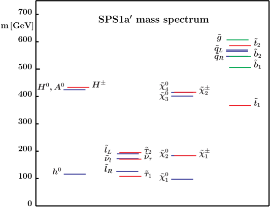
Figure A.1: Particle spectrum of the SPS1a’ parameter point.

Appendix B Comparison of EPA with the exact matrix element calculation

Photon-induced processes at linear colliders are commonly simulated using the equivalent photon approximation (EPA) [21]. The WHIZARD code allows one to use the exactly generated matrix element (cf. Sec. 2.4) and therefore provides means to test the quality of EPA. In the following we will expose the main differences between EPA and the exact matrix element calculations (EME). As an example we take the photon-induced tau-pair production process with successive leptonic tau decays.

Figure B.1: Lepton energy distributions from the photon-induced $\tau$ pair production processes (left: electron, right: muon) using the equivalent photon approximation (solid, black) and the exact matrix element (dotted, red).

Figure B.2: As Fig. B.1, but now plotting the difference between the EME and the rescaled EPA, $N^{\rm EME}_{i}-N_{i}^{\rm res}$. The 1-$\sigma$ error from the exact result is also given (dotted, red).

Process	preselno	no $p_{\perp}$3.33	no $E$3.33	no $\theta$3.33	no $\Delta\phi$no	all cuts
exact	787927	22685	10	14	867	10
EPA	767322	27974	–	–	1546	–

Table B.1: Comparison of cut efficiencies as in Table 4 for both EPA and exactly generated photon-induced $\tau$’s, normalized to 1 million events before preselection cuts.

The total cross section for photon-induced taus with their successive decay after preselection at 500 GeVare as follows:

$$\sigma_{\gamma\tau}^{\text{EPA}}\,=\,25.495(4)\,{\rm pb},\qquad\sigma_{\gamma\tau}^{\text{EME}}\,=\,21.392(70)\,{\rm pb},$$ (14)

so the EPA overestimates the number of generated taus. Figure B.1 shows the difference between lepton energy spectra generated with EPA and EME for electrons (left) and muons (right). The shapes of the distributions are roughly the same, so one may be tempted to account for the larger EPA distribution by a simple rescaling factor $K=\sigma^{\rm EME}/\sigma^{\rm EPA}$, i.e. taking $N_{i}^{\rm res}=K\,N_{i}^{\rm EPA}$ in the $i$-th bin. Figure B.2 shows the difference between EME and such rescaled EPA distributions demonstrating that the rescaled EPA clearly underestimates the number of low energy leptons. For investigations that rely on the lepton spectra at low energies this feature becomes crucial. In our analysis, some of the cuts were tailored to remove the low-energy leptons from photon-induced background, in particular the $p_{\perp}$ and $\Delta\phi$ cuts. Table B.1 shows the response of a sample of 10⁶ EPA and EME events each to the cuts. Employing the EPA instead of EME calculations would lead to an artificial reduction of the SM background by roughly 13%; for an integrated luminosity of 1 ab^-1 this corresponds to a 5$\sigma$ deviation from the expected SM background. It is therefore crucial to use the exact matrix elements in calculations of photon-induced processes.

References

- [1] Yu. A. Golfand and E. P. Likhtman, JETP Lett. 13, 323 (1971) [Pisma Zh. Eksp. Teor. Fiz. 13, 452 (1971)]; D. V. Volkov and V. P. Akulov, Phys. Lett. B 46, 109 (1973); J. Wess and B. Zumino, Phys. Lett. B 49, 52 (1974); Nucl. Phys. B 70, 39 (1974); for reviews see e.g. H. P. Nilles, Phys. Rept. 110, 1 (1984); H. E. Haber and G. L. Kane, Phys. Rept. 117, 75 (1985); D. J. H. Chung, L. L. Everett, G. L. Kane, S. F. King, J. D. Lykken and L. T. Wang, Phys. Rept. 407, 1 (2005) [arXiv:hep-ph/0312378].
- [2] G. L. Bayatian et al. [CMS Collaboration], CMS physics: Technical design report; J. Phys. G 34, 995 (2007); ATLAS detector and physics performance. Technical design report. Vol. 1+2; I. Hinchliffe, F. E. Paige, M. D. Shapiro, J. Soderqvist and W. Yao, Phys. Rev. D 55, 5520 (1997) [arXiv:hep-ph/9610544].
- [3] J. A. Aguilar-Saavedra et al. [ECFA/DESY LC Physics Working Group], arXiv:hep-ph/0106315; T. Abe et al. [American Linear Collider Working Group], Proc. of the APS/DPF/DPB Summer Study on the Future of Particle Physics (Snowmass 2001) ed. N. Graf, arXiv:hep-ex/0106056; K. Abe et al. [ACFA Linear Collider Working Group], arXiv:hep-ph/0109166; J. Brau et al., International Linear Collider reference design report, ILC-REPORT-2007-001, CERN-2007-006 (2007).
- [4] A. Freitas, W. Porod and P. M. Zerwas, Phys. Rev. D 72, 115002 (2005) [arXiv:hep-ph/0509056].
- [5] T. Robens, J. Kalinowski, K. Rolbiecki, W. Kilian and J. Reuter, Acta Phys. Pol. B 39, 1705 (2008) [arXiv:0803.4161 [hep-ph]].
- [6] J. A. Aguilar-Saavedra et al., Eur. Phys. J. C 46, 43 (2006) [arXiv:hep-ph/0511344].
- [7] B. C. Allanach et al., Eur. Phys. J. C 25, 113 (2002) [arXiv:hep-ph/0202233].
- [8] Y. Kato, K. Fujii, T. Kamon, V. Khotilovich and M. M. Nojiri, Phys. Lett. B 611, 223 (2005).
- [9] G. Weiglein et al. [LHC/LC Study Group], Phys. Rept. 426, 47 (2006) [arXiv:hep-ph/0410364].
- [10] E. Boos, G. A. Moortgat-Pick, H. U. Martyn, M. Sachwitz and A. Vologdin, arXiv:hep-ph/0211040; E. Boos, H. U. Martyn, G. A. Moortgat-Pick, M. Sachwitz, A. Sherstnev and P. M. Zerwas, Eur. Phys. J. C 30, 395 (2003).
- [11] H.U. Martyn, talk given at the ECFA/DESY Linear Collider workshop, Prague, November 2002, http://www-hep2.fzu.cz/ecfadesy/Talks/SUSY/, and LC-note LC-PHSM-2003-071; M. Dima et al., Phys. Rev. D 65, 071701 (2002).
- [12] W. Kilian, J. Reuter and T. Robens, Eur. Phys. J. C 48, 389 (2006); T. Robens, PhD thesis, 2006, arXiv:hep-ph/0610401.
- [13] T. Fritzsche and W. Hollik, Nucl. Phys. Proc. Suppl. 135, 102 (2004) [arXiv:hep-ph/0407095]; W. Oeller, H. Eberl and W. Majerotto, Phys. Rev. D 71, 115002 (2005) [arXiv:hep-ph/0504109].
- [14] K. Hagiwara et al., Phys. Rev. D 73, 055005 (2006); J. Reuter et al., arXiv:hep-ph/0512012; J. Reuter, arXiv:0709.0068 [hep-ph]; arXiv:0709.4638 [hep-ph].
- [15] J. A. Aguilar-Saavedra et al. [ECFA/DESY LC Physics Working Group], arXiv:hep-ph/0106315.
- [16] Z. Zhang, arXiv:0801.4888 [hep-ph].
- [17] http://whizard.event-generator.org; M. Moretti, T. Ohl, J. Reuter, hep-ph/0102195; W. Kilian, LC-TOOL-2001-039; W. Kilian, T. Ohl, J. Reuter, to appear in JHEP, arXiv:0708.4233 [hep-ph].
- [18] M. Beyer et al., Eur. Phys. J. C 48, 353 (2006); J. Reuter et al., arXiv:hep-ph/0512012; W. Kilian and J. Reuter, In the Proceedings of 2005 International Linear Collider Workshop (LCWS 2005), Stanford, California, 18-22 Mar 2005, pp 0311 [arXiv:hep-ph/0507099]. J. Reuter, PhD thesis, arXiv:hep-th/0212154; T. Ohl and J. Reuter, Eur. Phys. J. C 30, 525 (2003)
- [19] S. Jadach, Z. Was, R. Decker and J. H. Kuhn, Comput. Phys. Commun. 76, 361 (1993).
- [20] C. F. von Weizsäcker, Z. Phys. 88, 612 (1934); E. J. Williams, Phys. Rev. 45, 729 (1934).
- [21] V. M. Budnev, I. F. Ginzburg, G. V. Meledin and V. G. Serbo, Phys. Rept. 15, 181 (1974).
- [22] M. Skrzypek and S. Jadach, Z. Phys. C 49, 577 (1991).
- [23] T. Ohl, Comput. Phys. Commun. 101, 269 (1997) [arXiv:hep-ph/9607454].
- [24] LEPSUSYWG, ALEPH, DELPHI, L3 and OPAL experiments, note LEPSUSYWG/02-04.1, http://lepsusy.web.cern.ch/lepsusy/Welcome.html.
- [25] K. Desch, J. Kalinowski, G. Moortgat-Pick, K. Rolbiecki and W. J. Stirling, JHEP 0612, 007 (2006) [arXiv:hep-ph/0607104].
- [26] M. Rauch, R. Lafaye, T. Plehn and D. Zerwas, arXiv:0710.2822 [hep-ph]; R. Lafaye, T. Plehn and D. Zerwas, arXiv:hep-ph/0404282.
- [27] P. Bechtle, K. Desch and P. Wienemann, arXiv:hep-ph/0511137; P. Bechtle, K. Desch and P. Wienemann, In the Proceedings of 2005 International Linear Collider Workshop (LCWS 2005), Stanford, California, 18-22 Mar 2005, pp 0202 [arXiv:hep-ph/0506244]; P. Bechtle, K. Desch and P. Wienemann, Comput. Phys. Commun. 174, 47 (2006) [arXiv:hep-ph/0412012].
- [28] A. Datta, M. Guchhait and B. Mukhopadhyaya, Mod. Phys. Lett. A 10, 1011 (1995); A. Datta, M. Guchhait and M. Drees, Z. Phys. C 69, 347 (1996).
- [29] S. Y. Choi, A. Djouadi, M. Guchait, J. Kalinowski, H. S. Song and P. M. Zerwas, Eur. Phys. J. C 14, 535 (2000) [arXiv:hep-ph/0002033].
- [30] C. G. Lester, M. A. Parker and M. J. White, JHEP 0601, 080 (2006) [arXiv:hep-ph/0508143].
- [31] B. K. Gjelsten, D. J. Miller and P. Osland, JHEP 0412, 003 (2004) [arXiv:hep-ph/0410303].
- [32] J. Fujimoto, T. Ishikawa, Y. Kurihara, M. Jimbo, T. Kon and M. Kuroda, Phys. Rev. D 75, 113002 (2007); K. Rolbiecki, arXiv:0710.1748 [hep-ph]; K. Rolbiecki, PhD thesis, University of Warsaw 2008 (unpublished).
- [33] W. Porod, Comput. Phys. Commun. 153, 275 (2003) [arXiv:hep-ph/0301101].
- [34] M. Muhlleitner, A. Djouadi and Y. Mambrini, Comput. Phys. Commun. 168, 46 (2005) [arXiv:hep-ph/0311167].
- [35] G. Belanger, F. Boudjema, A. Pukhov and A. Semenov, Comput. Phys. Commun. 176, 367 (2007) [arXiv:hep-ph/0607059]; Comput. Phys. Commun. 174, 577 (2006) [arXiv:hep-ph/0405253]; Comput. Phys. Commun. 149, 103 (2002) [arXiv:hep-ph/0112278].