A non-Markovian decoherence theory for double dot charge qubit

Abstract

In this paper, we develop a non-perturbation theory for describing decoherence dynamics of electron charges in a double quantum dot gated by electrodes. We extend the Feynman-Vernon influence functional theory to fermionic environments and derive an exact master equation for the reduced density matrix of electrons in the double dot for a general spectral density at arbitrary temperature and bias. We then investigate the decoherence dynamics of the double dot charge qubit with back-action of the reservoirs being fully taken into account. Time-dependent fluctuations and leakage effects induced from the dot-reservoir coupling are explicitly explored. The charge qubit dynamics from the Markovian to non-Markovian regime is systematically studied under various manipulating conditions. The decay behavior of charge qubit coherence and the corresponding relaxation time $T_{1}$ and dephasing time $T_{2}$ are analyzed in details.

I Introduction

Double quantum dot systems have been attracting much attention because of their intriguing properties and their potential applications in nanotechnology and quantum information processing prs ; rmp . The basic structure of a double quantum dot system can be viewed as electrons confined in an electrostatic potential of double wells created by the fabricated gates, source and drain electrodes in the heterostructure of a semiconductor. The heterostructure of GaAs/AlGaAs is a typical example for the realization of gate-defined double dots. The tunability of various couplings and energy levels in the dots makes it a promising a quantum device (see, for examples, Elzerman ; hayashi ; petta ; Ludwig ; Gorman ). Maintaining electron coherence in a double quantum dot is an important ingredient in making it part of a quantum information processor. However, fluctuations and dissipations brought up by quantum operations of manipulations and measurements as well as various features of the material enrich the physics of double dot systems more than perfect coherent evolution. Thus a lot of attentions have been paid to investigate how various noises and interactions with the surroundings attenuate the coherent evolution of electrons in the double dot.

In this paper, we will concentrate on a non-perturbative dynamical theory for charge qubit manipulation with a double dot system gated by electrodes. In the quantum computing scheme in terms of double dots where the electron charge degree of freedom is exploited, the effects in deviating the coherency of charge dynamics are summarized in the fluctuations of the inter-dot coupling and energy splitting between the two local charge states as well as the dissipation induced damping effects. The amplitudes of these fluctuations can be estimated from measurements of the noise spectrum of electron currents and the minimum line width of elastic current peak prs . Parallel theoretical works have been developed with different approaches in the literature for the purposes of both simulating the experimental results and understanding the physical mechanisms living in the double dot. In the present work, we shall extend the Feynman-Vernon influence functional theory fv63 to fermionic environments and derive an exact master equation describing the coherent and decoherent dynamics of the electron charges in the double dot with the back-action effects of the reservoirs being fully taken into account.

Stochastic noise processes resulted in a time dependent Hamiltonian for the double dot have been widely analyzed in simulating the charge dynamics under noise influences. The Bloch-type rate equations for describing the double dot transport properties have been investigated by Gurvitz and co-worker Gurvitz used the many-body Schr$\ddot{\mbox{o}}$dinger equation approach which is further applied to study decoherence of double dot charge qubit in Fujisawa04 . The phonon assisted processes have been investigated within the Born-Markov regime by Brandes et al. using Born-Markov typed master equation tb . A general expression of the qubit density matrix in case of pure dephasing Palma was used by Fedichkin and Fedorov Fedorov to study the error rate of the charge qubit. Stavrou and Hu Stavrou considered in details the wavefunctions of the double dot charge qubit for decoherence analysis. Karrasch, et al. come with the functional renormalization group approach in dealing with the transport aspects of the multiple coupled dots ck . The non-Markovian dynamics has also recently been studied by a suitable spin-boson model considering the acoustic phonons by Thorwart, et al. using numerical quasiadiabatic propagator path integral scheme mt ; Liang . Without Born-Markov approximation, Wu et al. had devised an analytical expression for the dynamical tunneling current using a perturbation treatment based on a unitary transformation Wu ; xf . Effects from Coulomb interaction between the dots and the gate electrodes with the formulation of kinetic equations have been presented by Woodford et al. sr . The diversity in the methodologies and issues concerned in the literature show the physical richness of this novel system.

As we can see there are many factors competing to play the consequent physics in the double quantum dot system. To single out one factor from the others on the resulted dynamical properties of this charge device, we shall first concentrate in this paper on the effects induced by dot-reservoir coupling, where the double dot is designed in the strong Coulomb blockade regime such that each dot only contains one energy level. The reservoirs consist of the source and drain electrodes which are controllable through the bias voltage. A schematic plot of the system is shown in Fig. 1.

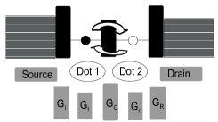
Figure 1: A schematic plot for the double quantum dot system

Thus the total Hamiltonian of the system we concern in this work is given by

$$H =E_{1}a^{\dagger}_{1}a_{1}+E_{2}a^{\dagger}_{2}a_{2}+T_{c}(a_{2}^{\dagger}a_{1}+a_{1}^{\dagger}a_{2})$$

$$~{}~{}~{}~{}~{}+\sum_{k}(\varepsilon_{Lk}a^{\dagger}_{Lk}a_{Lk}+\varepsilon_{Rk}a^{\dagger}_{Rk}a_{Rk})$$

$$~{}~{}~{}~{}~{}+\sum_{k}(t_{1Lk}a^{{\dagger}}_{1}a_{Lk}+t_{2Rk}a^{{\dagger}}_{Rk}a_{2}+{\rm H.c})$$ (1)

which contains the Hamiltonians of the double dot, the source and drain electrodes plus the interaction (electron tunneling processes) between them. The notations follow the convention and will be specified in details later.

Our treatment is based on the exact master equation we derived for a general spectral density of the electron reservoirs at arbitrary temperature and bias:

$$\dot{\rho}= -i[H^{\prime}(t),\rho]+\Gamma^{0}(t)\rho$$

$$+\sum_{ij}\Gamma_{ij}(t)(2a_{j}\rho a^{{\dagger}}_{i}-a^{{\dagger}}_{i}a_{j}\rho-\rho a^{{\dagger}}_{i}a_{j})$$

$$+\sum_{ij}\Gamma^{\beta}_{ij}(t)(a_{j}\rho a^{{\dagger}}_{i}-a^{{\dagger}}_{i}\rho a_{j}-a^{{\dagger}}_{i}a_{j}\rho-\rho a^{{\dagger}}_{i}a_{j}),$$ (2)

where $\rho$ is the reduced density matrix of the double dot obtained from the full density matrix of the double dot plus the reservoirs by tracing out the environmental degrees of freedom, and

$$H^{\prime}(t) =E^{\prime}_{1}(t)a^{{\dagger}}_{1}a_{1}+E^{\prime}_{2}(t)a^{{\dagger}}_{2}a_{2}+T^{\prime}_{c}(t)a^{{\dagger}}_{1}a_{2}+T^{\prime*}_{c}(t)a^{{\dagger}}_{2}a_{1}$$ (3)

is the corresponding effective Hamiltonian. All the time-dependent coefficients in the above equations will be derived explicitly and non-perturbatively in Sec. III. The time-dependent fluctuations of the energy levels, $E^{\prime}_{i}(t)$, and the inter-dot transition amplitude, $T^{\prime}_{c}(t)$, are the renormalization effects risen from the electron tunneling processes between the double dot and the reservoirs. Other non-unitary terms describe the dissipative and noise processes with time-dependent coefficients, $\Gamma^{0}(t),\Gamma(t)$ and $\Gamma^{\beta}(t)$, depicting the full non-Markovian decoherence dynamics. Eq. (2) is obtained without considering the inter-dot Coulomb repulsion. But as we will show explicitly in Sec. III it is easy to extend to the strong inter-dot Coulomb repulsion regime where the strong inter-dot Coulomb repulsion simply leads one to exclude the states corresponding to a simultaneous occupation of two dots from Eq. (2). Then the exact master equation allows us to exploit the intrinsic quantum decoherence effects in the electron charge coherency brought up by the tunneling processes between the dots and the reservoirs through the bias controls.

The master equation (2) is derived by extending the Feynman-Vernon influence functional theory fv63 to fermion coherent state path integrals wmz90 . Historically, since it was first developed by Feynman and Vernon in 1963 for quantum Brownian motion (QBM) modelled as a central harmonic oscillator linearly coupled to a set of harmonic oscillators simulating the thermal bath, the influence functional theory has been widely used to study dissipation dynamics in quantum tunneling problems legt and decoherence problems in quantum measurement theory zuk1 ; zuk . In these early applications, the master equation was derived for some particular class of ohmic environment cal ; hak ; uz89 . The exact master equation for the QBM with a general spectral density at arbitrary temperature was obtained by Hu and co-workers in 1992 hu . Applications of the QBM exact master equation cover various topics, such as quantum decoherence, quantum-to-classical transition and quantum measurement theory, etc.zuk . Very recently, such an exact master equation is further extended to the system of two entangled optical fields and two entangled harmonic oscillators for the study of non-Markovian entanglement dynamics in quantum information processing an07 ; chou08 . Nevertheless, using the influence functional theory to derive the exact master equation has been largely focused on the bosonic type of environments, up to date.

On the other hands, the development of quantum transport theory in nanosystems has continuously attracted attention in the last two decades because of the great achievements in nanotechnology, where the reservoir is, in many cases, a fermion system. The traditional approach to study the quantum transport in nanosystems is Schwinger-Keldysh’s nonequilibrium Green function formulism schwinger ; keldysh which has been extensively used in successfully describing various quantum transport phenomena, such as Kondo effect, Fano resonance and Coulomb blockade effects in quantum dots hers91 ; lee93 ; konig96 ; fuji03 . Master equations for quantum transport through quantum dots have also been derived, but mostly in the perturbation theory up to the second order brud91 ; leh02 ; ped05 ; li05 ; har06 . The exact master equation can be, in principle, obtained through the real-time diagrammatic expansion approach developed by Schön and co-workers schon94 ; konig96 , as shown recently by one of the authors and co-worker lee07 . Another interesting formulism is the recently published hierarchical expansion of the equations of motion for the reduced density matrix by Yan et. al. yan08 . Nevertheless, in contrast to the bosonic environments hu , an explicit formula of the exact master equation for fermionic environments with a general spectral density at arbitrary temperature and bias has not been carried out except for Eq. (2) in this work.

Unlike the quantum transport in nanosystems where people pay more attention on the tunneling current spectrum and its statistics, one cares in quantum information processing how the qubit coherency can be maintained for fast quantum operations where a strong coupling is required. Then a nonperturbative (with respect to the coupling between the system and its environment) master equation is more desirable for the precision manipulations of qubit states. Eq. (2) obtained in this paper has fully taken into account the back-action of the electron reservoirs at arbitrary temperature and bias. This master equation is also valid for a general spectral density. It is fully non-perturbative that goes far beyond the Born-Markovian approximation often used in the literature. It enables us to explore the dynamics of the electron charge coherence in the double dot, from Markovian to non-Markovian regime under various manipulating conditions. Many other approximated master equations that have been developed in the literature can be obtained at well defined limits of the present theory.

The rest of the paper is organized as follows. In the next section, we will use fermion-coherent-state path integral approach to solve exactly the electron dynamics in an isolated double quantum dots, as an illustration. We then extend the Feynman-Vernon influence functional theory originally built on the coordinate representation in quantum mechanics to fermion coherent state representation. The exact master equation for the reduced density matrix of the double dot system coupling to electron reservoirs is derived in Sec. III, where we also reproduce many other approximate master equations at well defined limits of the present formulae. In Sec. IV, we investigate the non-Markovian decoherence dynamics of this device including the tunneling induced fluctuations in the energy splitting and inter-dot coupling of the double dot as well as the noise and dissipation effects on the charge mode populations and interferences. The leakage effect is also discussed together there. The decay behaviors of charge qubit coherence and the corresponding relaxation time $T_{1}$ and dephasing time $T_{2}$ are analyzed in details. Conclusive remarks are given in Sec. V, and Appendices are presented for some detailed derivations.

II Fermion Coherent State Path Integral Approach to an isolated Double Dot

To illustrate the fermion coherent state path integral approach to the electron dynamics in a double quantum dot, we shall consider in this section a simple solvable system, a single electron in an isolated double dot, before we go to explore the realistic system in the next section. We also assume that each of the dots contains only one energy level, $E_{1}$ and $E_{2}$ respectively. The Hamiltonian of this isolated double quantum dot is

$$H=E_{1}a^{{\dagger}}_{1}a_{1}+E_{2}a^{{\dagger}}_{2}a_{2}+T_{c}(a_{2}^{\dagger}a_{1}+a_{1}^{\dagger}a_{2}).$$ (4)

The notations follow the convention: $a^{\dagger}_{1,2}$ are the creation operators for electrons in the double dot, and $T_{c}$ is the electron transition amplitude between the dots. In terms of the density operator, the time evolution of the system is described by

$$\rho(t)=U(t-t_{0})\rho(t_{0})U^{\dagger}(t-t_{0}),$$ (5)

where the density matrix $\rho(t)$ is the state of the system at a later time $t$, $\rho(t_{0})$ is the state at the initial time $t_{0}$, $U(t-t_{0})=\exp{\big{\{}-{i\over\hbar}H(t-t_{0})}\big{\}}$ is the evolution operator of the system, and we let $\hbar=1$ hereafter.

Using the fermion coherent state representation Faddeev , the density matrix at time $t$ is expressed as $\langle\xi|\rho(t)|\eta\rangle=\rho(\xi^{*},\eta,t)$ where $\xi$ and $\eta$ are two Grassmann variables characterizing the two-mode fermion coherent states,

$$|\xi\rangle=\prod_{i=1,2}|\xi_{i}\rangle~{},~{}~{}|\xi_{i}\rangle=\exp(-\xi_{i}a^{\dagger}_{i})|0\rangle,$$ (6)

The fermion coherent state defined above is an eigenstate of the fermion annihilation operator, $a_{i}|\xi_{i}\rangle=\xi_{i}|\xi_{i}\rangle$. As these coherent states are over-complete, they obey the resolution of identity, $\int d\mu(\xi)|\xi\rangle\langle\xi|=1,$ where the integration measure is defined by $d\mu(\xi)=\prod_{i}e^{-\xi^{*}_{i}\xi_{i}}d\xi^{*}_{i}d\xi_{i}$. Note that the fermionic coherent states we used here are not normalized, and the normalization factors are moved into the above integration measure. Moreover, these coherent states are also nonorthogonal. The overlap of two fermionic coherent states is: $\langle\xi|\xi^{\prime}\rangle=\exp(\xi^{\dagger}\xi^{\prime})$ with a matrix notation $\xi^{\dagger}=(\xi^{*}_{1}~{}\xi^{*}_{2})$.

The use of the coherent-state representation makes the path integral formulation for a fermion system generally possible. In the fermionic coherent-state representation, the time evolution of the density matrix becomes

$$\rho(\xi_{f}^{*},\eta_{f},t)=\int d\mu(\xi_{0})d\mu(\eta_{0})\rho(\xi_{0}^{*},\eta_{0},t_{0})$$

$$\times J(\xi_{f}^{*},\eta_{f},t|\xi_{i}0,\eta^{*}_{0},t_{0}),$$ (7)

where $J(\xi_{f}^{*},\eta_{f},t|\xi_{0},\eta^{*}_{0},t_{0})=\langle\xi_{f}|U(t-t_{0})|\xi_{0}\rangle\langle\eta_{0}|U^{\dagger}(t-t_{0})|\eta_{f}\rangle$ is the propagating function in which the forward and backward transition amplitudes $\langle\xi_{f}|U(t-t_{0})|\xi_{0}\rangle$ and $\langle\eta_{0}|U^{\dagger}(t-t_{0})|\eta_{f}\rangle$ can be solved exactly using the path integral for the Hamiltonian (4).

Explicitly, the fermion coherent state path integral for the forward transition amplitude is given by

$$\langle\xi_{f}|U(t-t_{0})|\xi_{0}\rangle=\int\mathcal{D}[\xi,\xi^{*}]\exp\big{(}iS_{c}[\xi^{*},\xi]\big{)},$$ (8)

where the action is

$$S_{c}[\xi^{*},\xi]=\sum_{i=1,2}\Big{\{}-{i\over 2}\big{[}\xi^{*}_{if}\xi_{i}(t)+\xi^{*}_{i}(t_{0})\xi_{i0}\big{]}~{}~{}~{}~{}~{}~{}~{}~{}~{}$$

$$~{}~{}~{}+\int_{t_{0}}^{t}d\tau\big{[}{i\over 2}(\xi^{*}_{i}\dot{\xi}_{i}-\dot{\xi}_{i}^{*}\xi_{i})-(E_{i}\xi^{*}_{i}\xi_{i}+T_{c}\xi^{*}_{i}\xi_{i^{\prime}})\big{]}\Big{\}}.$$ (9)

In the above equation, the path integral $\mathcal{D}[\xi,\xi^{*}]$ integrates over all pathes $\xi_{i}(\tau)$ and $\xi^{*}_{i}(\tau)$ bounded by $\xi_{i}(t_{0})=\xi_{i0}$ and $\xi^{*}_{i}(t)=\xi^{*}_{if}$ with $i\neq i^{\prime}$. Since the action in Eq. (8) has a quadratic form, the path integral can be exactly carried out with the stationary path method fey65 ; Faddeev . The result is

$$\langle\xi_{f}|U(t-t_{0})|\xi_{0}\rangle=\exp{\sum_{i}\Big{[}{\xi^{*}_{if}\xi_{i}(t)+\xi_{i}^{*}(t_{0})\xi_{i0}\over 2}\Big{]}},$$ (10)

where $\xi_{i}^{*}(t_{0})$ and $\xi_{i}(t)$ are determined by the solution of the equations of motion

$$\dot{\xi}_{i}(\tau)+i\big{[}E_{i}\xi_{i}(\tau)+T_{c}\xi_{i^{\prime}}(\tau)\big{]} =0,$$ (11a)

$$\dot{\xi}^{*}_{i}(\tau)-i\big{[}E_{i}\xi^{*}_{i}(\tau)+T_{c}\xi^{*}_{i^{\prime}}(\tau)\big{]} =0,$$ (11b)

with the boundary conditions $\xi_{i}(t_{0})=\xi_{i0}$ and $\xi^{*}_{i}(t)=\xi^{*}_{if}$, where $i\neq i^{\prime}$. The backward transition amplitude $\langle\eta_{0}|U^{\dagger}(t-t_{0})|\eta_{f}\rangle$ can be found by the same procedure. From Eq. (11) we can introduce a $2\times 2$ matrix $u_{0}(t)$ such that $\xi(t)=u_{0}(t)\xi_{0}$ and $\xi^{\dagger}(t_{0})=\xi^{\dagger}_{f}u_{0}(t)$ where $u_{0}(t)$ satisfies the equation of motion

$$\dot{u_{0}}(t)+i\begin{pmatrix}E_{1}&T_{c}\\ T_{c}&E_{2}\end{pmatrix}u_{0}(t)=0$$ (12)

with the boundary condition $(u_{0})_{ij}(t_{0})=\delta_{ij}$. The solution of (12) is:

$$u_{0}(t)=e^{-i\phi(t)}(\cos\varphi(t)I-i{\bf n}\cdot\boldsymbol{\sigma}\sin\varphi(t))$$ (13)

with $\phi(t)=E(t-t_{0})$, $\varphi(t)=\Omega_{0}(t-t_{0})/2$. Here we have also defined $E\equiv{1\over 2}(E_{1}+E_{2})$ and the Rabi frequency $\Omega_{0}=\sqrt{\varepsilon^{2}+\Delta^{2}}$, where $\varepsilon\equiv E_{1}-E_{2}$ is the energy level splitting in the double dot and $\Delta=2T_{c}$ the inter-dot tunnel coupling. $\boldsymbol{\sigma}$ is the Pauli matrix, $I$ a $2\times 2$ identity matrix and the unit vector ${\bf n}\equiv(\Delta,0,\varepsilon)/\Omega_{0}$. Then the propagating function becomes

$$J(\xi_{f}^{*},\eta_{f},t|\xi_{0},\eta^{*}_{0},t_{0})=\exp{(\xi^{{\dagger}}_{f}u_{0}(t)\xi_{0}+\eta^{{\dagger}}_{0}u_{0}^{{\dagger}}(t)\eta_{f})}.$$ (14)

If we use further the D-algebra of fermion creation and annihilation operators in the fermion coherent state representation $|\xi\rangle$ wmz90 ,

$$\xi_{i}|\xi\rangle=a_{i}|\xi\rangle~{},~{}~{}-{\partial\over\partial\xi_{i}}|\xi\rangle=a^{\dagger}_{i}|\xi\rangle,$$ (15a)

$$\langle\xi|\xi^{*}_{i}=\langle\xi|a^{\dagger}_{i}~{},~{}~{}\langle\xi|{\partial\over\partial\xi^{*}_{i}}=\langle\xi|a_{i},$$ (15b)

it is easy to derive the equation of motion for the density operator $\rho(t)$:

$$\dot{\rho}(t)=\sum_{ij}\Big{\{}[ \dot{u_{0}}(t)u_{0}(t)^{-1}]_{ij}a^{{\dagger}}_{i}a_{j}\rho(t)$$

$$+[\dot{u_{0}}(t)u_{0}(t)^{-1}]^{*}_{ij}\rho(t)a^{{\dagger}}_{j}a_{i}\Big{\}}.$$ (16)

One can see from Eq. (12) that $\dot{u_{0}}(t)u_{0}(t)^{-1}=-i\begin{pmatrix}E_{1}&T_{c}\\ T_{c}&E_{2}\end{pmatrix}$. This simply reduces Eq. (16) to the familiar Liouvillian equation,

$$\dot{\rho}(t)=-i[H,\rho(t)],$$ (17)

as we expected. Having ensured the path integral technique can reproduce the dynamical equation for an isolated double quantum dot, we will apply it to the double quantum dot coupling to electron reservoirs in the next section.

III The Master Equation for a Double Quantum Dot Gated by Electrodes

A double quantum dot between two electron reservoirs, the source and drain electrodes controlled via a bias voltage (see Fig. 1), has a total Hamiltonian as

$$H = H_{\rm dot}+H_{\rm rev}+H_{I},$$ (18)

where

$$H_{\rm dot}=E_{1}a^{\dagger}_{1}a_{1} +E_{2}a^{\dagger}_{2}a_{2}+T_{c}(a_{2}^{\dagger}a_{1}+a_{1}^{\dagger}a_{2})$$ (19a)

is the Hamiltonian of the double quantum dots,

$$H_{\rm rev}=\sum_{k}(\varepsilon_{Lk}a^{\dagger}_{Lk}a_{Lk}+\varepsilon_{Rk}a^{\dagger}_{Rk}a_{Rk})$$ (19b)

is for the source and drain electrodes (reservoirs) and

$$H_{I}=\sum_{k}(t_{1Lk}a^{{\dagger}}_{1}a_{Lk}+t_{2Rk}a^{{\dagger}}_{Rk}a_{2}+{\rm H.c})$$ (19c)

is the coupling (interaction) between the double dot and the reservoirs that depicts the electron tunneling between them, where subscript $k$ labels an electron state in the reservoirs, $L$ and $R$ denote the reservoirs of the source (left) and drain (right) electrodes, respectively, and $t_{1Lk}(t_{2Rk})$ is the electron tunneling amplitude between the source (drain) and the left (right) dot. Since we only concern in this work the dynamics of charge qubit, we omitted spin degrees of freedom for electrons.

It should be pointed out that in Eq. (19a) we did not include explicitly the inter-dot Coulomb repulsion. This is because a typical inter-dot Coulomb energy is of the order of hundreds $\mu$eV, which is much larger than the energy level splitting $\varepsilon$ and the inter-dot tunnel coupling $\Delta$ (both are of the order of tens $\mu$eV or less) for charge qubit manipulation hayashi . As a result, the inter-dot Coulomb interaction simply leads one to exclude the states corresponding to a simultaneous occupation of the two dots tb ; Gurvitz . Thus, we will derive an exact master equation for the reduced density matrix of the double dot without considering the inter-dot Coulomb repulsion at beginning. The master equation of the double dot in the strong inter-dot Coulomb repulsion regime is then obtained from the exact master equation by explicitly excluding the states of doubly occupied two dots in terms of Bloch-type rate equations, as we will see later.

To derive non-puterbatively the master equation of the reduced density matrix for the double dot system, we adopt the treatment of the Feynman-Vernon influence functional theory fv63 . This approach within the framework of path integral traces over the degrees of freedom of the environment (here the electrodes) into a functional of the dynamical variables of the system (the double quantum dot). This functional is called the influence functional by Feynman and Vernon, which contains all the dynamical effects from the back-action of the reservoirs to the system due to the coupling between them. Following the fermionic path integral technique presented in the last section, we depict the route to an exact master equation aided with the results derived in details in the appendices.

III.1 Influence functional

Explicitly, the total density matrix of the double dot plus the reservoirs obeys the quantum Liouvillian equation $i\partial\rho_{\mathrm{tot}}(t)/\partial t=[H,\rho_{\mathrm{tot}}(t)]$, which yields the formal solution:

$$\rho_{\mathrm{tot}}(t)=e^{-iH(t-t_{0})}\rho_{\mathrm{tot}}(t_{0})e^{iH(t-t_{0})}.$$ (20)

As we are interested in dynamics of the electrons in the double dot, we shall concentrate on the reduced density matrix for the double dot by tracing out the environmental variables: $\rho(t)={\rm tr}_{E}\rho_{\rm{tot}}(t)$. Assuming initially the dots and the reservoirs are uncorrelated legt ; hu , $\rho_{\mathrm{tot}}(t_{0})=\rho(t_{0})\otimes\rho_{E}(t_{0})$, then the reduced density matrix describing the full dynamics of the electrons in the double dot becomes

$$\langle\xi_{f}|\rho(t)|\eta_{f}\rangle=\int d\mu(\xi_{0}) d\mu(\eta_{0})\langle\xi_{0}|\rho(t_{0})|\eta_{0}\rangle$$

$$\times J(\xi_{f}^{*},\eta_{f},t|\xi_{0},\eta_{0}^{*},t_{0}),$$ (21)

where the propagating function is defined as

$$J(\xi_{f}^{*}, \eta_{f},t|\xi_{0},\eta_{0}^{*},t_{0})=$$

$$\int\mathcal{D}[\xi^{*}\xi;\eta^{*}\eta]e^{i(S_{c}[\xi^{*},~{}\xi]-S^{*}_{c}[\eta^{*},~{}\eta])}\mathcal{F}[\xi^{*}\xi;\eta^{*}\eta]$$ (22)

with $S_{c}[\xi^{*},\xi]$ being the action of the double dot in the fermion coherent state representation given by Eq. (9), and $\mathcal{F}[\xi^{*}\xi;\eta^{*}\eta]$ is the influence functional which takes fully into account the back-action effects of the reservoirs to the double dot and modifies the original action of the system into an effective one, $e^{{i\over\hbar}(S_{c}[\xi^{*},\xi]-S^{*}_{c}[\eta^{*},\eta])}\mathcal{F}[\xi^{*}\xi;\eta^{*}\eta]=e^{{i\over\hbar}S_{eff}[\xi^{*}\xi;\eta^{*}\eta]}$. The path integral $\mathcal{D}[\xi^{*}\xi;\eta^{*}\eta]$ integrates over all pathes $\xi^{*}(\tau),\xi(\tau),\eta^{*}(\tau)$, and $\eta(\tau)$ in the Grassmann space bounded by $\xi^{*}(t)=\xi^{*}_{f}$, $\xi(t_{0})=\xi_{0}$, $\eta^{*}(t_{0})=\eta^{*}_{0}$, and $\eta(t)=\eta_{f}$.

Let the reservoirs be initially in thermal equilibrium states at temperature $\beta^{-1}$, the influence functional can then be solved exactly with the result (see the derivation in the Appendix A):

$$\mathcal{F}[\xi^{*}\xi;\eta^{*}\eta]= \exp\sum_{i=1,2}\Big{\{}-\int_{t_{0}}^{t}d\tau\int_{t_{0}}^{\tau}d\tau^{\prime}\Big{(}F_{il}(\tau-\tau^{\prime})\xi^{*}_{i}(\tau)\xi_{i}(\tau^{\prime})+F^{*}_{il}(\tau-\tau^{\prime})\eta^{*}_{i}(\tau^{\prime})\eta_{i}(\tau)\Big{)}$$

$$+\int_{t_{0}}^{t}d\tau\int_{t_{0}}^{t}d\tau^{\prime}\Big{(}F_{il}(\tau-\tau^{\prime})\eta^{*}_{i}(\tau)\xi_{i}(\tau^{\prime})-F_{il}^{\beta}(\tau-\tau^{\prime})\big{(}\eta^{*}_{i}(\tau)+\xi^{*}_{i}(\tau)\big{)}\big{(}\eta_{i}(\tau^{\prime})+\xi_{i}(\tau^{\prime})\big{)}\Big{)}\Big{\}}.$$ (23)

The two time correlation functions in the influence functional,

$$F_{il}(\tau-\tau^{\prime})=\sum_{k}|t_{ilk}|^{2}e^{-i\varepsilon_{lk}(\tau-\tau^{\prime})},$$ (24a)

$$F_{il}^{\beta}(\tau-\tau^{\prime})=\sum_{k}f(\varepsilon_{lk})|t_{ilk}|^{2}e^{-i\varepsilon_{lk}(\tau-\tau^{\prime})},$$ (24b)

are called the dissipation-fluctuation kernels, where $f(\varepsilon_{lk})={1\over e^{\beta(\varepsilon_{lk}-\mu_{l})}+1}$ with $l=L,R$ for $i=1,2$, respectively, are the fermi distribution functions of the electron reservoirs, and $\mu_{L,R}$ are the corresponding chemical potentials. These nonlocal time-dependent functions contains the full dynamics effect from the reservoirs to the double dot. We should also point out that in the coherent state representation, the influence functional for a many-fermion environment has a form similar to that of a many-boson environment an07 except for some sign difference due to the antisymmetric properties of fermion degrees of freedom.

The physical meaning of the above influence functional is very clear. The four terms contained in the exponential function of Eq. (23) correspond to four different physical processes in a time-closed path formulism, see Fig. 2.

Figure 2: The closed-time path for the trace of the density matrix of the reservoirs.

The first term gives the contribution of the back-action effect of the reservoirs to the double dot in terms of the time correlation function $F_{il}(\tau-\tau^{\prime})$ of Eq. (24a) in the forward process from the time $t_{0}$ to the time $t$. For the double time integrals it contains, the first one starts from $t_{0}$ to $\tau$ and the second one from $t_{0}$ to $t$, sums over all the time sequences of the these propagations. Resummation of these propagating processes up to all orders of the system-reservoir coupling results in exactly the exponential function appearing in Eq. (23). Similar to the first term, the second term are just the back-action effect of the reservoirs to the system in the backward process from the time $t$ back to the time $t_{0}$ which is just the complex conjugate of the first term. In terms of the Schwinger-Keldysh Green-function approach, the time correlation function in these two propagating processes are just the time-ordered and anti-time ordered Green functions. The histories of the forward pathes $\xi^{*}_{i}(\tau),\xi_{i}(\tau)$ and the backward pathes $\eta^{*}_{i}(\tau),\eta_{i}(\tau)$ are mixed up through the time correlation functions as shown in the third and the fourth terms in Eq. (23). The third term in Eq. (23) represents the mix of the forward and backward pathes at the time $t$. The last term is a mix of the forward and backward pathes at the time $t_{0}$ where the initial equilibrium properties of the reservoirs, i.e. the fermi statistics and the temperature of the reservoirs, naturally enter into the time correlation function $F_{il}^{\beta}(\tau-\tau^{\prime})$, as shown by Eq. (24b).

As we see all the influences of the reservoirs on the double dot are embedded in the two time-correlation functions, i.e., the two dissipation-fluctuation kernels (24) in the influence functional. These two dissipation-fluctuation kernels are related each other through the dissipation-fluctuation theorem. This will become clear by introducing a spectral density defined as

$$J_{il}(\omega)=\sum_{k}|t_{ilk}|^{2}\delta(\omega-\varepsilon_{lk}).$$ (25)

Obviously, the spectral density contains all the information about the reservoirs’ density of states involved in the electron tunneling between the dots and reservoirs. Then the time-correlation functions (24) can be expressed as

$$F_{il}(\tau-\tau^{\prime})=\int d\omega J_{il}(\omega)e^{-i\omega(\tau-\tau^{\prime})},$$ (26a)

$$F_{il}^{\beta}(\tau-\tau^{\prime})=\int d\omega{J_{il}(\omega)e^{-i\omega(\tau-\tau^{\prime})}\over e^{\beta(\omega-\mu_{l})}+1},$$ (26b)

This equation manifests the dissipation-fluctuation theorem in an open quantum system. It tells that all the back-action effects of the reservoirs to the double dot are crucially determined by the spectral density $J_{il}(\omega)$.

III.2 Exact master equation

Now we can derive the master equation for the reduced density matrix. As we see the effective action after integrating out the environmental degrees of freedom, i.e. combining Eqs. (22) and (23) together, still has a quadratic form in terms of the dynamical variables of the fermion coherent states. Thus the path integral (22) can be solved exactly by utilizing the stationary path method and gaussian integrals fey65 ; Faddeev . The resulting propagating function is simply given by

$$J(\xi_{f}^{*},\eta_{f},t|\xi_{0},\eta_{0}^{*},t_{0})=A(t)\exp\sum_{i=1,2}\Big{[}{\xi^{*}_{if}\xi_{i}(t)+\xi^{*}_{i}(t_{0})\xi_{i0}\over 2}+{\eta^{*}_{i0}\eta_{i}(t_{0})+\eta^{*}_{i}(t)\eta_{if}\over 2}\Big{]}.$$ (27)

where $A(t)$ is the contribution arisen from the fluctuations around the stationary pathes which will be given later. The stationary pathes $\xi_{i}(t)$ and $\eta_{i}(t_{0})$ are determined by the equations of motion

$$\dot{\xi}_{i}(\tau)+i[E_{i}\xi_{i}(\tau)+T_{c}\xi_{i^{\prime}}(\tau)]+\int_{t_{0}}^{\tau}d\tau^{\prime}F_{il}(\tau-\tau^{\prime})\xi_{i}(\tau^{\prime}) -\int_{t_{0}}^{t}d\tau^{\prime}F_{il}^{\beta}(\tau-\tau^{\prime})[\xi_{i}(\tau^{\prime})+\eta_{i}(\tau^{\prime})]=0$$ (28a)

$$\dot{\eta}_{i}(\tau)+i[E_{i}\eta_{i}(\tau)+T_{c}\eta_{i^{\prime}}(\tau)]+\int_{t_{0}}^{\tau}d\tau^{\prime}F_{il}(\tau-\tau^{\prime})\eta_{i}(\tau^{\prime}) -\int_{t_{0}}^{t}d\tau^{\prime}F_{il}(\tau-\tau^{\prime})[\eta_{i}(\tau^{\prime})+\xi_{i}(\tau^{\prime})]$$

$$+\int_{t_{0}}^{t}d\tau^{\prime}F_{il}^{\beta}(\tau-\tau^{\prime})[\eta_{i}(\tau^{\prime})+\xi_{i}(\tau^{\prime})]=0$$ (28b)

subjected to the boundary condition $\xi_{i}(t_{0})=\xi_{i0}$ and $\eta_{i}(t)=\eta_{if}$, while $\xi^{*}_{i}(t_{0})$ and $\eta^{*}_{i}(t)$ in Eq. (27) can be obtained from the complex conjugate equations of (28b) and (28a), respectively, under the boundary condition $\xi^{*}_{i}(t)=\xi^{*}_{if}$ and $\eta^{*}_{i}(t_{0})=\eta^{*}_{i0}$. The local terms $\dot{\xi}_{i}+i(E_{i}\xi_{i}+T_{c}\xi_{i^{\prime}})$ and $\dot{\eta}_{i}+i(E_{i}\eta_{i}+T_{c}\eta_{i^{\prime}})$ in Eq. (28) are intrinsic and well describe the coherent dynamics of the electron states in an isolated double quantum dot, as we have discussed in the last section. The nonlocal terms involving two different time correlation functions, $F_{il}(\tau-\tau^{\prime})$ and $F_{il}^{\beta}(\tau-\tau^{\prime})$, stem from the coupling to the reservoirs. These two time correlation functions play quite distinct roles in the equations of motion. The interaction between the double dot and the electron reservoirs is mediated through electron tunnelings between them. The correlation $F_{il}(\tau-\tau^{\prime})$ describes the back-action of the reservoirs to the double dot due to the interaction between them. However, the correlation function $F_{il}^{\beta}(\tau-\tau^{\prime})$ also harbors the Fermi-Dirac statistic effect of the electron reservoirs which exists even in the zero-temperature limit. The latter situation is quite different from a bosonic environment where $F_{il}^{\beta}(\tau-\tau^{\prime})$ vanishes at zero temperature an07 .

The solutions of $\xi_{i}(t)$, $\eta_{i}(t_{0})$ and $\eta^{*}_{i}(t)$, $\xi^{*}_{i}(t_{0})$ determined by Eq. (28) and its complex conjugate can be factorized from the corresponding boundary conditions. It is not too difficult to find that

$$\xi(t)=(I-v(t))^{-1}\big{[}u(t)\xi_{0}+v(t)\eta_{f}\big{]},~{}$$ (29a)

$$\eta(t_{0})=u^{{\dagger}}(t)[I+(I-v(t))^{-1}v(t)]\eta_{f}$$

$$~{}~{}~{}~{}~{}~{}~{}~{}~{}~{}~{}~{}~{}~{}-\big{[}I-u^{\dagger}(t)(I-v(t))^{-1}u(t)\big{]}\xi_{0}.$$ (29b)

Here we have again used the matrix notation: $\xi^{T}=(\xi_{1}~{}\xi_{2})$ and a same form for $\eta$. The new dynamical variables expressed as two time-dependent $2\times 2$ matrices, $u(\tau)$ and $v(\tau)$, satisfy the dissipation-fluctuation integrodifferential equations:

$$\dot{u}(\tau)+iMu(\tau)+\int^{\tau}_{t_{0}} d\tau^{\prime}G(\tau-\tau^{\prime})u(\tau^{\prime})=0,$$ (30a)

$$\dot{v}(\tau)+iMv(\tau)+\int_{t_{0}}^{\tau} d\tau^{\prime}G(\tau-\tau^{\prime})v(\tau^{\prime})$$

$$=\int_{t_{0}}^{t}d\tau^{\prime}G^{\beta}(\tau-\tau^{\prime})\bar{u}(\tau^{\prime}),$$ (30b)

with the boundary conditions $u_{ij}(t_{0})=\delta_{ij}$ and $v_{ij}(t_{0})=0$, while $\bar{u}(\tau)$ in Eq. (30b) obeys the backward equation of motion to $u(\tau)$, namely, $\bar{u}(\tau)=u^{\dagger}(t+t_{0}-\tau)$ for $t_{0}\leq\tau\leq t$. In Eq. (30), we have also defined the $2\times 2$ matrices $M_{ij}=E_{i}(i=j)$ and $T_{c}(i\neq j)$, $G_{ij}(\tau-\tau^{\prime})=F_{il}(\tau-\tau^{\prime})\delta_{ij}$, and $G^{\beta}_{ij}(\tau-\tau^{\prime})=F_{il}^{\beta}(\tau-\tau^{\prime})\delta_{ij}$. As we see $u(\tau)$ is determined purely by $F_{il}(\tau-\tau^{\prime})$ while $v(\tau)$ depends on both correlation functions. The full complexity of the non-Markovian dynamics of charge coherence in the double dot induced from its coupling to the reservoirs is thus manifested through these equations of motion.

As $\xi^{*}_{i}(t_{0})$ and $\eta^{*}_{i}(t)$ satisfying respectively the complex conjugate equations of $\eta_{i}(\tau)$ and $\xi_{i}(\tau)$ with the boundary condition $\xi^{*}_{i}(t)=\xi^{*}_{if}$ and $\eta^{*}_{i}(t_{0})=\eta^{*}_{i0}$, it is easy to find the similar solution from Eq. (29) for $\xi^{*}_{i}(t_{0})$ and $\eta^{*}_{i}(t)$. Substituting these results into Eq. (27) and note the fact that $v(\tau)$ is a hermitian matrix at $\tau=t$, we obtain explicitly the exact propagating function of the double dot system:

$$J(\xi^{*}_{f},\eta_{f},t| \xi_{0},\eta^{*}_{0},t_{0})=A(t)\exp\Big{\{}\xi^{\dagger}_{f}J_{1}(t)\xi_{0}$$

$$+\xi^{\dagger}_{f}J_{2}(t)\eta_{f}+\eta^{\dagger}_{0}J_{3}(t)\xi_{0}+\eta^{\dagger}_{0}J^{\dagger}_{1}(t)\eta_{f}\Big{\}},$$ (31)

where

$$J_{1}(t)=w(t)u(t),~{}~{}J_{2}(t)=w(t)-I,$$ (32a)

$$J_{3}(t)=u^{{\dagger}}(t)w(t)u(t)-I,~{}~{}A(t)=1/{\rm det}(w(t)).$$ (32b)

with $w(t)=(I-v(t))^{-1}$. All these time-dependent coefficients can be fully determined by solving Eq. (30).

Once the exact propagating function is obtained, the dynamics of the reduced density matrix, Eq. (21), which takes fully into account the back-action of the electron reservoirs, can be completely solved for any given initial electron state of the double dot. The explicit solution of the reduced density matrix relies solely on the solution to the equations of motion (30) which, in general, has to be solved numerically. To check the consistency, we may let the double dot be decoupled from the electron reservoirs, namely, set $t_{ilk}=0$, then the dissipation-fluctuation kernels vanish. As a result, Eq. (30a) is reduced to Eq. (12) and $u(t)$ is reduced to $u_{0}(t)$ whose solution is given after Eq. (12) in the last section, while the solution of Eq. (30b) gives $v(t)=0$. Consequently the propagating function Eq. (31) is reduced to Eq. (14) which recovers the exact solution of the isolated double dot system shown in the last section.

Having the explicit form of the propagating function (31) in hands, it is straightforward to derive the master equation for the reduced density matrix directly from Eq. (21). Here we shall deduce an operator form of the master equation such that all the time-dependent coefficients in the master equation are explicitly independent from the initial state of the double dot as well as from any specific representation. Taking the time derivative to Eq. (31), eliminating the initial state dependence and using the D-algebra of the fermion creation and annihilation operators in the fermion coherent state representation, Eq.(15), the exact master equation of the double dot with a general spectral density at arbitrary temperature and bias is given by:

$$\dot{\rho}(t)= \sum_{ij}\Big{\{}\Omega_{ij}(t)[a^{\dagger}_{i}a_{j},\rho(t)]$$

$$+\Gamma_{ij}(t)(2a_{j}\rho(t)a^{{\dagger}}_{i}-a^{{\dagger}}_{i}a_{j}\rho(t)-\rho(t)a^{{\dagger}}_{i}a_{j})$$

$$+\Gamma^{\beta}_{ij}(t)(a_{j}\rho(t)a^{{\dagger}}_{i}-a^{{\dagger}}_{i}\rho(t)a_{j}-a^{{\dagger}}_{i}a_{j}\rho(t)-\rho(t)a^{{\dagger}}_{i}a_{j})\Big{\}}$$

$$+\Gamma^{0}(t)\rho(t),$$ (33)

where all time-dependent coefficients in Eqs. (33) are determined by $u(t)$ and $v(t)$ through the following relations:

$$\Omega_{ij}(t)={1\over 2}[\dot{u}u^{-1}-(u^{\dagger})^{-1}\dot{u}^{\dagger}]_{ij},$$ (34a)

$$\Gamma_{ij}(t)=-{1\over 2}[\dot{u}u^{-1}+(u^{\dagger})^{-1}\dot{u}^{\dagger}]_{ij},$$ (34b)

$$\Gamma^{\beta}_{ij}(t)=[\dot{u}u^{-1}v+v(u^{\dagger})^{-1}\dot{u}^{\dagger}-\dot{v}]_{ij},$$ (34c)

and $\Gamma^{0}(t)={\rm tr}\Gamma^{\beta}$. The first term in the master equation is indeed the generalized Liouvillian term which can be explicitly written as

$$\sum_{ij}\Omega_{ij}(t)[a^{\dagger}_{i}a_{j},\rho]=-i[H^{\prime}(t),\rho]$$ (35)

where

$$H^{\prime}(t) =E^{\prime}_{1}(t)a^{{\dagger}}_{1}a_{1}+E^{\prime}_{2}(t)a^{{\dagger}}_{2}a_{2}+{T^{\prime}_{c}(t)}a^{{\dagger}}_{1}a_{2}+{T^{\prime*}_{c}(t)}a^{{\dagger}}_{2}a_{1}$$ (36)

is an effective Hamiltonian of the double quantum dot with the shifted (renormalized) time-dependent energy levels and the shifted inter-dot transition amplitude,

$$E^{\prime}_{i}(t)=i\Omega_{ii}~{}~{}(i=1,2),~{}~{}~{}T^{\prime}_{c}(t)=i\Omega_{12}.$$ (37a)

Using the equation of motion (30a), we further obtain

$$E^{\prime}_{i}(t)=E_{i}-\mbox{Im}[W_{ii}(t)],~{}~{}i=1,2,$$ (37b)

$$T^{\prime}_{c}(t)=T_{c}+{i\over 2}[W_{12}(t)-W^{*}_{21}(t)],$$ (37c)

where

$$W(t)=\int_{t_{0}}^{t}d\tau\begin{pmatrix}F_{1L}(t-\tau)&0\\ 0&F_{2R}(t-\tau)\end{pmatrix}u(\tau)u(t)^{-1},$$ (37d)

It shows that the shifted energy levels, $E^{\prime}_{1,2}(t)$, and the inter-dot transition amplitude, $T^{\prime}_{c}(t)$, are entirely contributed by $u(t)$ that involves only the time-correlation function $F_{il}(t-\tau)$. The rest part in Eq. (33) describes the dissipation and noise processes of electron charges with non-Markovian behaviors having been embedded in these time-dependent $2\times 2$ matrix coefficients, $\Gamma(t)$ and $\Gamma^{\beta}(t)$. We call $\Gamma(t)$ and $\Gamma^{\beta}(t)$ the dissipation-fluctuation matrix coefficients or simply the dissipation-fluctuation coefficients hereafter. Note that $\Gamma(t)$ is solely determined by $u(t)$, and $\Gamma^{\beta}(t)$ is given by both $u(t)$ and $v(t)$. Thus all the time-dependent coefficients in the master equation are non-perturbatively determined by Eq. (30) and fully account the back-action effects of the reservoirs to the double dot.

III.3 Bloch-type Rate equations for zero and strong inter-dot Coulomb repulsion cases and the corresponding Markovian limits

(a) No inter-dot Coulomb repulsion: To closely examine the decoherence of electron charge dynamics in the double dot, it is more convenient to rewrite the master equation (33) as a set of Bloch-type rate equations in terms of the localized charge states in the double dot. Without considering the inter-dot Coulomb repulsion, the rate equations can be obtained directly from the master equation (33) in the charge configuration space containing the states of empty double dot, the first dot occupied, the second dot occupied and both dots occupied. We label these four states by $|j\rangle,j=0,1,2,3$, respectively. Then the master equation in the above basis becomes

$$\dot{\rho}_{00} =\tilde{\Gamma}_{11}\rho_{11}+\tilde{\Gamma}_{21}\rho_{12}+\tilde{\Gamma}_{12}\rho_{21}+\tilde{\Gamma}_{22}\rho_{22}+\Gamma^{0}\rho_{00},$$ (38a)

$$\dot{\rho}_{11} =(\Gamma^{0}-2\bar{\Gamma}_{11})\rho_{11}+\bar{\Xi}^{*}_{-}\rho_{12}+\bar{\Xi}_{-}\rho_{21}$$

$$~{}~{}~{}~{}~{}~{}~{}~{}~{}~{}~{}~{}~{}~{}~{}~{}~{}~{}~{}~{}~{}~{}~{}~{}~{}~{}-\Gamma^{\beta}_{11}\rho_{00}+\tilde{\Gamma}_{22}\rho_{33},$$ (38b)

$$\dot{\rho}_{22} =(\Gamma^{0}-2\bar{\Gamma}_{22})\rho_{22}+\bar{\Xi}^{*}_{+}\rho_{12}+\bar{\Xi}_{+}\rho_{21}$$

$$~{}~{}~{}~{}~{}~{}~{}~{}~{}~{}~{}~{}~{}~{}~{}~{}~{}~{}~{}~{}~{}~{}~{}~{}~{}~{}-\Gamma^{\beta}_{22}\rho_{00}+\tilde{\Gamma}_{11}\rho_{33},$$ (38c)

$$\dot{\rho}_{12} =[-i\varepsilon^{\prime}+\Gamma^{0}-{\rm tr}\bar{\Gamma}]\rho_{12}+\bar{\Xi}_{+}\rho_{11}+\bar{\Xi}_{-}\rho_{22}$$

$$~{}~{}~{}~{}~{}~{}~{}~{}~{}~{}~{}~{}~{}~{}~{}~{}~{}~{}~{}~{}~{}~{}~{}~{}~{}~{}-\Gamma^{\beta}_{12}\rho_{00}+\tilde{\Gamma}_{12}\rho_{33},$$ (38d)

$$\dot{\rho}_{33} =\Gamma^{\beta}_{12}\rho_{21}+\Gamma^{\beta}_{21}\rho_{12}-\Gamma^{\beta}_{11}\rho_{22}-\Gamma^{\beta}_{22}\rho_{11}$$

$$~{}~{}~{}~{}~{}~{}~{}~{}~{}~{}~{}~{}~{}~{}~{}~{}~{}~{}~{}~{}~{}~{}~{}~{}~{}~{}+(\Gamma^{0}-2{\rm tr}\bar{\Gamma})\rho_{33}.$$ (38e)

Here the density matrix elements are defined by $\rho_{ij}=\langle i|\rho|j\rangle$. We have also defined all the time-dependent coefficients in the rate equations as $\tilde{\Gamma}(t)=2\Gamma(t)+\Gamma^{\beta}(t)$, $\bar{\Gamma}(t)=\Gamma(t)+\Gamma^{\beta}(t)$, $\bar{\Xi}_{\pm}=\pm iT^{\prime}_{c}(t)-\bar{\Gamma}_{12}$ and $\varepsilon^{\prime}(t)=E^{\prime}_{1}(t)-E^{\prime}_{2}(t)$ where $E^{\prime}_{i}(t),T^{\prime}_{c}(t),\Gamma(t),\Gamma^{\beta}(t)$ and $\Gamma^{0}(t)$ are the time-dependent transport coefficients contained in the master equation and are explicitly given by Eqs. (34) and (37). These time-dependent coefficients in the rate equations thus fully characterize the non-Markovian dynamics of electrons in the double dot. The first and the last rate equations account electron charge leakage effects in this device, while other three rate equations depict charge qubit decoherence dynamics under the influence of the reservoirs.

For a constant spectral density that has been widely used in the literature, the time-correlation function becomes

$$F_{il}(\tau-\tau^{\prime})\rightarrow{\Gamma_{l}\over 2\pi}\int_{-\infty}^{\infty}d\omega e^{-i\omega(\tau-\tau^{\prime})}=\Gamma_{l}\delta(\tau-\tau^{\prime}),$$ (39)

where $\Gamma_{l}=2\pi\rho_{l}|t_{ilk}|^{2}$, ($l=L,R$ for $i=1,2$), and $\rho_{L,R}$ are the densities of states for the left and right electron reservoirs. Then in the Markovian limit ($t-t_{0}$, $\tau-t_{0}\rightarrow\infty$) Carmichael93 , the integral kernels in Eq. (30) reduce to

$$\int_{t_{0}}^{\tau}d\tau^{\prime}F_{il}(\tau-\tau^{\prime})u_{ij}(\tau^{\prime})\rightarrow{1\over 2}\Gamma_{l}u_{ij}(\tau),$$ (40a)

$$\int_{t_{0}}^{t}d\tau^{\prime}F^{\beta}_{il}(\tau-\tau^{\prime})\bar{u}_{ij}(\tau^{\prime})\rightarrow f_{l}\Gamma_{l}\bar{u}_{ij}(\tau).$$ (40b)

The factor ${1\over 2}$ in Eq.(40a) comes from the boundary of the time integration sitting upon $\tau$, and $f_{L,R}$ in Eq. (40b) are the fermi distribution functions of the reservoirs. In this Markovian limit, the equation of motion (30) can be solved analytically and the solution is

$$u(\tau)=\exp\Big{\{}-\begin{pmatrix}iE_{1}+{\Gamma_{L}\over 2}&iT_{c}\\ iT_{c}&iE_{2}+{\Gamma_{R}\over 2}\end{pmatrix}(\tau-t_{0})\Big{\}},$$ (41a)

$$v(\tau)=\int_{t_{0}}^{\tau}d\tau^{\prime}u(\tau+t_{0}-\tau^{\prime})\begin{pmatrix}f_{L}\Gamma_{L}&0\\ 0&f_{R}{\Gamma_{R}}\end{pmatrix}\bar{u}(\tau^{\prime}+t_{0}).$$ (41b)

With the above explicit solution for $u(t)$ and $v(t)$, we can obtain analytically all the coefficients in the master equation as well. Note that $\bar{u}(\tau)=u^{\dagger}(t+t_{0}-\tau)$ depending explicitly on the time $t$ implies that $\partial_{\tau}v(\tau)|_{\tau=t}\neq\partial_{t}v(t)=\dot{v}(t)$, it is easy to find

$$\dot{u}u^{-1}=-\begin{pmatrix}iE_{1}+{\Gamma_{L}\over 2}&iT_{c}\\ iT_{c}&iE_{2}+{\Gamma_{R}\over 2}\end{pmatrix},$$ (42a)

$$\dot{u}u^{-1}v+v(u^{\dagger})^{-1}\dot{u}^{\dagger}-\dot{v}=-\begin{pmatrix}f_{L}\Gamma_{L}&0\\ 0&f_{R}{\Gamma_{R}}\end{pmatrix}.$$ (42b)

As a result, for a constant spectral density in the Markovian limit, all the time-dependent coefficients in the master equation become constant:

$$E^{\prime}_{1,2}(t)\rightarrow E_{1,2},~{}~{}T^{\prime}_{c}(t)\rightarrow T_{c},$$ (43a)

$$\Gamma_{ij}(t)\rightarrow{1\over 2}\Gamma_{l}\delta_{ij},~{}~{}\Gamma^{\beta}_{ij}(t)\rightarrow-f_{l}\Gamma_{l}\delta_{ij}.$$ (43b)

In other words, in the Markovian limit with a constant spectral density, there is no renormalization effect to the energy level shift and the inter-dot transition amplitude. The dissipation-fluctuation effects are simply reduced to the time-independent tunneling rates between the dots and the reservoirs. In fact, the differences of time-dependent and time-independent coefficients manifest the non-Markovian dynamics of electron charges in the double dot. We shall present quantitatively such differences in the next section.

For a constant spectral density in the Markovian limit, the rate equations are simply reduced to

$$\dot{\rho}_{00} =\bar{f}_{L}\Gamma_{L}\rho_{11}+\bar{f}_{R}\Gamma_{R}\rho_{22}-(f_{L}\Gamma_{L}+f_{R}\Gamma_{R})\rho_{00},$$ (44a)

$$\dot{\rho}_{11} =-(\bar{f}_{L}\Gamma_{L}+f_{R}\Gamma_{R})\rho_{11}+iT_{c}(\rho_{12}-\rho_{21})$$

$$~{}~{}~{}~{}~{}~{}~{}~{}~{}~{}~{}~{}~{}~{}+f_{L}\Gamma_{L}\rho_{00}+\bar{f}_{R}\Gamma_{R}\rho_{33},$$ (44b)

$$\dot{\rho}_{22} =-(\bar{f}_{R}\Gamma_{R}+f_{L}\Gamma_{L})\rho_{22}-iT_{c}(\rho_{12}-\rho_{21})$$

$$~{}~{}~{}~{}~{}~{}~{}~{}~{}~{}~{}~{}~{}~{}+f_{R}\Gamma_{R}\rho_{00}+\bar{f}_{L}\Gamma_{L}\rho_{33},$$ (44c)

$$\dot{\rho}_{12} =(-i\varepsilon-{\Gamma_{L}+\Gamma_{R}\over 2})\rho_{12}+iT_{c}(\rho_{11}-\rho_{22}),$$ (44d)

$$\dot{\rho}_{33} =-(\bar{f}_{L}\Gamma_{L}+\bar{f}_{R}\Gamma_{R}]\rho_{33}+f_{L}\Gamma_{L}\rho_{22}+f_{R}\Gamma_{R}\rho_{11},$$ (44e)

where $\bar{f}_{L,R}=(1-f_{L,R})$ and $\varepsilon=E_{1}-E_{2}$. Under the large bias limit, $f_{L}=1,~{}f_{R}=0$, the above rate equations reproduce the rate equations obtained by Gurvitz and Prager Gurvitz for the double dot without considering the inter-dot Coulomb repulsion:

$$\dot{\rho}_{00}=-\Gamma_{L}\rho_{00}+\Gamma_{R}\rho_{22},$$ (45a)

$$\dot{\rho}_{11}=\Gamma_{L}\rho_{00}+\Gamma_{R}\rho_{33}+iT_{c}(\rho_{12}-\rho_{21}),$$ (45b)

$$\dot{\rho}_{22}=-(\Gamma_{L}+\Gamma_{R})\rho_{22}-iT_{c}(\rho_{12}-\rho_{21}),$$ (45c)

$$\dot{\rho}_{12}=(-i\varepsilon-{\Gamma_{L}+\Gamma_{R}\over 2})\rho_{12}+iT_{c}(\rho_{11}-\rho_{22}),$$ (45d)

$$\dot{\rho}_{33}=-\Gamma_{R}\rho_{33}+\Gamma_{L}\rho_{22}.$$ (45e)

(b) Strong inter-dot Coulomb repulsion: On the other hand, realistic experiments of the double dot are set up in the strong Coulomb blockade regime where not only each of dots has only one effective energy level but also there is no states of simultaneous occupation of the two dots. In other words, the configuration space of the localized charge states in the double dot system with a strong inter-dot Coulomb repulsion only contains the states of empty double dot, the first dot occupied and the second dot occupied, denoted by $|j\rangle,j=0,1,2,$ respectively. The corresponding rate equations in this strong Coulomb blockade regime for an arbitrary spectral density can also be obtained by simply excluding the doubly occupied states in Eq. (38). Since the rate of the doubly occupied state $|3\rangle$ in the case of ignoring inter-dot Coulomb repulsion depends on the populations $\rho_{11}$ and $\rho_{22}$. This probability flow from the states $|1\rangle$ and $|2\rangle$ to $|3\rangle$ should be redirected back into the states $|1\rangle$ and $|2\rangle$ in the strong inter-dot Coulomb repulsion regime. Meanwhile, to ensure the probability conservation without the doubly occupied states, a correction to the dependence of the coherence elements $\rho_{12}$ and $\rho_{21}$ in the rate equations for $\rho_{11}$ and $\rho_{22}$ must also be taken into account guided by the condition:

$$\Gamma^{\beta}_{12}\rho_{21}+\Gamma^{\beta}_{21}\rho_{12}-\Gamma^{\beta}_{11}\rho_{22}-\Gamma^{\beta}_{22}\rho_{11}=0.$$ (46)

This condition indeed forces the doubly occupied state to decouple from other states in the double dot, as one can see from the rate equation $\dot{\rho}_{33}$ in Eq. (38). These modifications can be done explicitly by taking the following shift to the coefficients in the non-interacting rate equations (38): $\bar{\Gamma}_{ii}\rightarrow\bar{\Gamma}_{ii}+{1\over 2}\Gamma^{\beta}_{jj}$, $\bar{\Gamma}_{ij}\rightarrow\bar{\Gamma}_{ij}-{1\over 2}\Gamma^{\beta}_{ij}$ with $i\neq j$. In fact, the above coefficient shift also automatically cancels the $\Gamma^{0}$ dependence of $\rho_{33}$ in Eq. (38), which is indeed a criterion for entirely excluding the double occupied state from the reduced density matrix, as one can directly see from the expression of the master equation (33). Then the rate equation of $\rho_{33}$ in Eq. (38) becomes $\dot{\rho}_{33}=(-2{\rm tr}\bar{\Gamma})\rho_{33}$, its solution is $\rho_{33}(t)=0$ if initially $\rho_{33}(t_{0})=0$. This implies that no leakage into the double occupied state will occur. As a result, the rate equations in the strong inter-dot Coulomb repulsion regime are given by

$$\dot{\rho}_{00} =\tilde{\Gamma}_{11}\rho_{11}+\tilde{\Gamma}_{21}\rho_{12}+\tilde{\Gamma}_{12}\rho_{21}+\tilde{\Gamma}_{22}\rho_{22}+\Gamma^{0}\rho_{00},$$ (47a)

$$\dot{\rho}_{11} =-\tilde{\Gamma}_{11}\rho_{11}+\tilde{\Xi}^{*}_{-}\rho_{12}+\tilde{\Xi}_{-}\rho_{21}-\Gamma^{\beta}_{11}\rho_{00},$$ (47b)

$$\dot{\rho}_{22} =-\tilde{\Gamma}_{22}\rho_{22}+\tilde{\Xi}^{*}_{+}\rho_{12}+\tilde{\Xi}_{+}\rho_{21}-\Gamma^{\beta}_{22}\rho_{00},$$ (47c)

$$\dot{\rho}_{12} =[-i\varepsilon^{\prime}-{1\over 2}{\rm tr}\tilde{\Gamma}]\rho_{12}+\tilde{\Xi}_{+}\rho_{11}+\tilde{\Xi}_{-}\rho_{22}-\Gamma^{\beta}_{12}\rho_{00},$$ (47d)

where $\tilde{\Xi}_{\pm}(t)=\pm iT^{\prime}_{c}(t)-{1\over 2}\tilde{\Gamma}_{12}(t)$. This set of the rate equations depicts the full non-Markovian dynamics of the double dot in the strong inter-dot Coulomb repulsion regime.

For the case of a constant spectral density in the Markovian limit, $\tilde{\Gamma}_{ij}(t)=(2\Gamma(t)+\Gamma^{\beta}(t))_{ij}\rightarrow\bar{f}_{l}\Gamma_{l}\delta_{ij}$, $\tilde{\Xi}_{\pm}(t)\rightarrow\pm iT_{c}$ and $\varepsilon^{\prime}(t)\rightarrow\varepsilon$. The rate equations under such circumstances are reduced to the rate equations for the double dot in the strong inter-dot Coulomb repulsion regime, given in tb ,

$$\dot{\rho}_{00}=-(f_{L}\Gamma_{L}+f_{R}\Gamma_{R})\rho_{00}+\bar{f}_{L}\Gamma_{L}\rho_{11}+\bar{f}_{R}\Gamma_{R}\rho_{22},$$ (48a)

$$\dot{\rho}_{11}=f_{L}\Gamma_{L}\rho_{00}+iT_{c}(\rho_{12}-\rho_{21})-\bar{f}_{L}\Gamma_{L}\rho_{11},$$ (48b)

$$\dot{\rho}_{22}=f_{R}\Gamma_{R}\rho_{00}-iT_{c}(\rho_{12}-\rho_{21})-\bar{f}_{R}\Gamma_{R}\rho_{22},$$ (48c)

$$\dot{\rho}_{12}=\big{[}-i\varepsilon-{1\over 2}(\bar{f}_{L}\Gamma_{L}+\bar{f}_{R}\Gamma_{R})\big{]}\rho_{12}+iT_{c}(\rho_{11}-\rho_{22}).$$ (48d)

Furthermore, in the large bias limit, $f_{L}=1,~{}f_{R}=0$, the above rate equations lead to Stoof-Nazarov’s rate equations Stoof :

$$\dot{\rho}_{00}=-\Gamma_{L}\rho_{00}+\Gamma_{R}\rho_{22},$$ (49a)

$$\dot{\rho}_{11}=\Gamma_{L}\rho_{00}+iT_{c}(\rho_{12}-\rho_{21}),$$ (49b)

$$\dot{\rho}_{22}=-\Gamma_{R}\rho_{22}-iT_{c}(\rho_{12}-\rho_{21}),$$ (49c)

$$\dot{\rho}_{12}=(-i\varepsilon-{\Gamma_{R}\over 2})\rho_{12}+iT_{c}(\rho_{11}-\rho_{22}).$$ (49d)

In a summary, we have derived in this section an exact master equation for the double dot gated by electrodes, and the corresponding Bloch-type rate equations (38) without considering the inter-dot Coulomb interaction as well as the rate equations (47) for the strong inter-dot Coulomb repulsion. For convenience, we call Eq. (38) the interaction-free rate equations and Eq. (47) the strong-interaction rate equations hereafter. Other approximated rate equations that have been used in the literature are obtained at well defined limit of the present formulae.

IV Non-Markovian dynamics of charge qubit

With the above formulae we can now systematically explore the non-Markovian dynamics of the charge qubit for this double dot system. The coherence (decoherence) dynamics of electron charges in the double dot is determined by its internal structure as well as external operations. The internal structure includes the spectral properties of the reservoirs as well as the couplings between the dots and the reservoirs embedded in the spectral density. The external operations include charge qubit initialization, its coherence manipulation and the qubit state readout through the bias controls of the source and drain electrodes. Non-Markovian decoherence effects of these internal structure and external operations to the charge qubit are manifested through the time-dependent coefficients in the master equation, which is completely determined by Eq. (30) after the spectral density $J_{il}(\omega)$ is specified. In fact, the time correlation functions directly tell us the length of the correlation time which determines to what extent the time-dependent fluctuation and memory effect become important. The longer the correlation time is, the more memory effect acts on the electron dynamics in the double dot and vice versa.

To be more specific, we should first specify the spectral density $J_{il}(\omega)$ for the source and drain electrodes. Unlike the bosonic environment where a general spectral density $J(\omega)=\eta\omega\Big{(}\frac{\omega}{\omega_{c}}\Big{)}^{n-1}e^{-\frac{\omega}{\omega_{c}}}$ ($\omega_{c}$ is a high frequency cutoff and $\eta$ is a dimensionless coupling constant) was defined and used to classify the bosonic environment as Ohmic if $n=1$, sub-Ohmic if $0<n<1$, and super-Ohmic for $n>1$ legt , for a fermionic environment a general spectral density should not be a Poisson or Gaussian type distribution function because of the fermi statistics. Here we shall use a Lorentzian spectral density that has been used in the study of the influence of a measuring lead on a single dot Elattari and molecular wires coupling to electron reservoirs Welack . The Lorentzian spectral density we used here has a form:

$$J_{il}(\omega)={\Gamma_{l}d_{l}^{2}/2\pi\over(\omega-E_{i})^{2}+{d_{l}}^{2}},$$ (50)

where $E_{i}$ is chosen to be the energy levels of the double dot, and $l=L,R$ for $i=1,2$, respectively. There are two parameters in $J_{il}(\omega)$ that characterize the time scales of the reservoirs. The parameters $d_{L,R}$ describe the widths of the Lorentzian distributions, which tell how many states in the reservoirs around $E_{1,2}$ effectively involve in the electron tunneling between the reservoirs and dots. Hence, the inverse $d_{L,R}^{-1}$ characterize the time scales of the source and drain electrodes. Another parameter is the electron tunneling strength or the tunneling rate between the reservoirs and dots, $\Gamma_{L,R}$, its inverse characterizes the time scale of the electron tunneling process itself between the reservoirs and dots. Indeed, $\Gamma_{L,R}$ also describe leakage effects of electrons from dots to the reservoirs and vice versa. Thus a Lorentzian spectral density well depict the time scales of non-Markovian processes in this open quantum system.

Also, the choice of a Lorentzian spectral density makes it easy to recover the constant spectral density which has been often used in the literature. In fact, taking the large width limit, namely assuming all the electron states in the reservoirs has an equal possibility for electron tunneling between the reservoir and dot, then $2\pi J_{il}(\omega)\stackrel{{\scriptstyle\longrightarrow}}{{{}_{{}_{d_{l}\rightarrow\infty}}}}\Gamma_{l}$ reproduces the constant spectral density that has often been used in the study of both quantum transport and quantum decoherence phenomena in nanostructures. In this limit, the time scale of the reservoirs is suppressed. Furthermore, in the previous investigations, especially in the study of quantum transport phenomena, one also takes a long time limit. Combining these two limits (the constant spectral density and long time limit) together, the exact master equation is reduced to the Bloch-type rate equations in the Markovian approximation obtained by others tb ; Stoof ; Gurvitz , as we have shown in the last section. Hence, with a Lorentzian spectral density, it is not only convenient to analyze in details the non-Markovian dynamics but also enables us to easily make a comparison with the Markovian dynamics.

For a Lorentzian spectral density, the corresponding temperature-independent time correlation function can be exactly calculated. The result is

$$F_{il}(\tau-\tau^{\prime})={\Gamma_{l}d_{l}\over 2}\exp\big{\{}-(d_{l}+iE_{i})|\tau-\tau^{\prime}|\big{\}}.$$ (51)

Obviously, $d_{L,R}^{-1}$ describes the correlation times of the reservoirs. The wider/narrower it is, the shorter/longer the correlation time will be. The internal structure of the double dot is characterized by the energy level splitting $\varepsilon=E_{1}-E_{2}$ and the inter-dot tunnel coupling $\Delta=2T_{c}$, its time scale $T_{0}$ is given by the inverse of the bare Rabi frequency $\Omega_{0}=\sqrt{\varepsilon^{2}+\Delta^{2}}$. The non-Markovian dynamics should be dominated when the two typical time scales, $\Omega_{0}^{-1}$ and $d_{L,R}^{-1}$, are in the same order of magnitude. There is another time scale, the reservoirs’ temperature $\beta=1/kT$ that also influences the non-Markovian dynamics of the charge qubit in certain cases. In the current experiments for charge qubit manipulation hayashi , the temperature is roughly fixed at 100 mK. We will take this temperature throughout our analysis to the charge qubit decoherence.

IV.1 Time dependent coefficients in the master equation and non-Markovian dynamics

Once the spectral density is specified, the full non-Markovian dynamics of charge qubit in the double dot can be depicted using the master equation (33), or more specifically the corresponding Bloch-type rate equations (38) and (47) for the cases of no inter-dot Coulomb repulsion and strong inter-dot Coulomb repulsion double dot, respectively. To solve the master equation or equivalently the rate equations, we must determine first the time-dependent coefficients contained in these equations, namely the shifted (renormalized) energy level splitting $\varepsilon^{\prime}(t)=E^{\prime}_{1}(t)-E^{\prime}_{2}(t)$ and inter-dot tunneling coupling $\Delta^{\prime}(t)=2T^{\prime}_{c}(t)$, as well as the dissipation-fluctuation coefficients $\Gamma(t)$ and $\Gamma^{\beta}(t)$. These transport coefficients are completely determined by the functions $u(t)$ and $v(t)$ as the solutions of the dissipation-fluctuation equations of motion (30) which have to be solved numerically for a given spectral density.

Using the Lorentzian spectral density (50), we can calculate explicitly all the time-dependent transport coefficients in the master equations and then discuss the corresponding non-Markovian dynamics by comparing with the Markovian limit in various different time scales. We shall first analyze the time-dependent coefficients for the charge qubit initialization where a bias is applied to the double dot and the double dot is adjusted to be off-resonance, i.e. $eV_{SD}=\mu_{L}-\mu_{R}\neq 0$ and $\varepsilon=E_{1}-E_{2}\neq 0$ hayashi . We will examine when the large bias limit is reached and how the initialization works. After that we will go to the coherent manipulation regime where the double dot is set up symmetrically ($E_{1}=E_{2}$) and the chemical potentials of the electron reservoirs are aligned above the energy levels of two dots with zero bias voltage ($\mu_{L}=\mu_{R}$). The time dependence of $\varepsilon^{\prime}(t),T^{\prime}_{c}(t)$ as well as $\Gamma(t)$ and $\Gamma^{\beta}(t)$ in this regime will tell us when the non-Markovian dynamics becomes important during the charge qubit evolution.

The dissipation-fluctuation equations of motion (30) show that only the solution of $v(t)$ depends on the fermi distribution function in the reservoirs. In other words, only $\Gamma^{\beta}(t)$ sensitively depends on the bias. Other coefficients, $\varepsilon^{\prime}(t),T^{\prime}_{c}(t)$ and $\Gamma(t)$, do not depend on the chemical potentials $\mu_{L,R}$ and thus the bias. Their time dependencies are completely determined by the internal parameters of the double dot and the spectral density. In the initialization scheme where a bias is presented and the energy splitting of the two levels in the double dot is nonzero within the transport window, the time-dependence of $\Gamma^{\beta}$ is plotted in Fig. 3 by varying the bias voltage. We find that the large bias limit is reached at about 100 $\mu$eV for the given internal parameters $\varepsilon=30~{}\mu$eV, $\Delta=10\mu$eV, $\Gamma_{L,R}=\Delta$ and $d_{L,R}=\Delta/2$, with $\Omega_{0}=\sqrt{\varepsilon^{2}+\Delta^{2}}\simeq 32\mu$eV being the bare Rabi frequency of the charge qubit. This large bias limit is shown in Fig. 3 that the curves for $eV_{SD}=90~{}\mu$eV are very close to the curves of $eV_{SD}=430~{}\mu$eV, and the curves for $eV_{SD}=130~{}\mu$eV perfectly overlap with the curves of $eV_{SD}=430~{}\mu$eV.

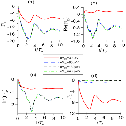
Figure 3: The time-dependence of $\Gamma^{\beta}$ by varying the bias voltage. The double dot is set to be off-resonance with $\varepsilon=30~{}\mu$eV, $\Delta=10\mu$eV, $\Gamma_{L,R}=\Delta$ and $d_{L,R}=\Omega_{0}/2$. (a) and (d) show the two diagonal matrix elements of $\Gamma^{\beta}$. Since $\Gamma^{\beta}$ is hermitian only one of the off-diagonal elements is plotted with the real part shown in (b) and the imaginary part in (c). The period of the bare Rabi cycle is $T_{0}=2\pi/\Omega_{0}$.

Fig. 4 shows the time-dependence of other coefficients for different energy level splitting of the double dot states ($\varepsilon=0,10,70\mu$eV) with different tunneling rate ($\Gamma_{L}=\Gamma_{R}=2.5,10,25\mu$eV). The result shows that $\varepsilon^{\prime}(t)=0$ for $\varepsilon=0$, and the initial value $\mbox{Re}(T_{c}^{\prime})(0)$ always equals to $T_{c}$ with $\mbox{Im}(T^{\prime}_{c})(0)$ being zero in all the cases we have calculated. For a small tunneling rate ($\Gamma_{L,R}<\Delta/2$), the time-dependence of these coefficients is almost negligible (see red solid lines in Fig. 4). The time-dependent effect appears when the tunneling rates between the reservoirs and dots become relatively large. These time-dependent behaviors vary sensitively on the energy splitting of the double dot states. Increasing the energy splitting $\varepsilon$ changes the time-dependent behaviors of all the coefficients significantly, as shown in Fig 4.

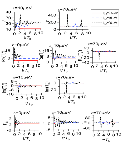
Figure 4: The time-dependence of the coefficients $\varepsilon^{\prime}(t),T^{\prime}_{c}(t)$ and $\Gamma(t)$ for different energy splitting $\varepsilon$ and tunneling rate $\Gamma_{L,R}$ at the inter-dot coupling $\Delta=10\mu$eV and the spectral widthes $d_{L,R}=\Delta/2$.

The dynamics of electron charges in this initialization regime is plotted in Fig. 5. If we dope only one excess electron in the left dot with the right dot being empty, the efficiency of keeping this initial state decreases as the bias decreasing [see Fig. 5(a)]. If the two levels of the double dot are in resonance ($\varepsilon=0$) or the inter-dot tunnel coupling is larger than the tunneling rates $\Delta>2\Gamma_{L,R}$, it also has a low efficiency to keep the double dot in the initial state $\rho_{11}=1$. A large bias configuration ($eV_{SD}$ larger than 100 $\mu$eV) maintains the double dot in the initial state $\rho_{11}=1$ very well. Furthermore, for a large bias it also quickly leads the double dot into the state $\rho_{11}\thicksim 1$ even if the initial state is $\rho_{00}=1$ (both dots are empty initially) or $\rho_{22}=1$(the left dot is empty but the right dot is occupied by one excess electron), as shown in Fig. 5(b). These numerical solutions are obtained using the interaction-free rate equations (38). But the strong-interaction rate equations (47) give qualitatively the same result for initialization. Taking the bias to be 650$\mu$eV and the reservoirs’ temperature to be 100mK that have used in experiments hayashi , a very efficient initialization of the charge qubit can be obtained, as shown in Fig. 5.

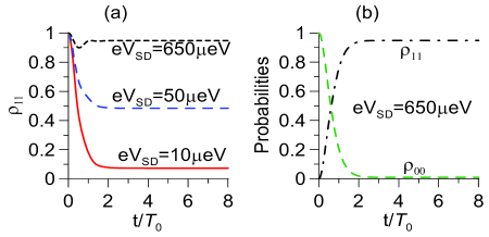
Figure 5: (a) The time evolution of $\rho_{11}$, the probability of finding one excess electron in the left dot with the right dot being empty, is plotted at various bias when the initial state is $\rho_{11}=1$. (b) The time evolutions of $\rho_{11}$(black dash-dotted line) and $\rho_{00}$(green long dashed line) when the initial state is an empty state ($\rho_{00}=1$), where $eV_{SD}=650\mu$eV. Other input parameters used here are the same as that in Fig. 3.

Meanwhile, Fig. 4 shows that for a relatively large tunneling rate $\Gamma_{L,R}$, the smooth time oscillation of all the coefficients at small $\varepsilon$ become discontinuing at a relatively large $\varepsilon$ value. Such discontinuities correspond to the electron hopping to the localized charge states in the double dot where the inter-dot tunnel coupling $\Delta$ is almost negligible in comparison with the level splitting $\varepsilon$. Such discontinuities are also manifested perfectly in the electron dynamics. The discontinuities coincide with the times at which the electron is found in a localized charge state of the double dot in a very high probability. Fig. 6(a)-(b) are obtained using the rate equations (38) and (47), respectively, where we plot the corresponding electron charge dynamics together with the time-dependence of $\Gamma_{11}$. We find that for a large bias, the electron charge dynamics given by the interaction-free rate equations (38) and the strong-interaction rate equations (47) display the same feature, including the coincidence between the discontinuities in the time-dependent coefficients and the emergence of a localized charge state in the double dot. Note that if a sufficiently large bias is applied across the double dot, initialization can still be achieved regardless of these discontinuities. This is because a large bias is the most dominant factor in this situation. As a conclusion, initialization of charge qubit in the double dot can be easily achieved in a large bias limit with relatively small tunnel coupling and tunneling rates. All these parameters are tunable in experiments.

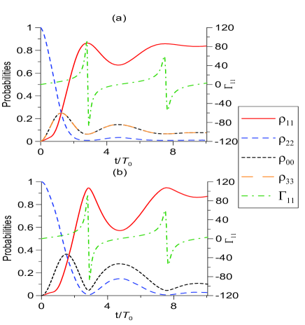
Figure 6: The coincidence between the discontinuities in $\Gamma_{11}(t)$ (the green dot-dashed line) and the emergence of a localized charge state in the double dot. The input parameters $\varepsilon=70\mu$eV, $\Delta=10\mu$eV, $d_{L,R}=\Delta/2$ and $\Gamma_{L,R}=25\mu$eV with the bias $eV_{SD}=120\mu$eV such that the initialization can be achieved. (a) for the double dot without considering the inter-dot Coulomb repulsion. (b) for the double dot in the strong inter-dot Coulomb repulsion regime.

Now we turn into the regime for charge qubit rotations where the double dot is set up at the resonant levels ($E_{1}=E_{2}=E$) and the fermi surfaces of the electron reservoirs are aligned above the resonant levels ($\mu_{L}=\mu_{R}=\mu$ and $\mu-E>0$). In other words, the double dot is set to be symmetric and unbiased for charge coherence manipulation hayashi . Figs. 7-9 show the time-dependencies of the shifted inter-dot tunnel coupling $\Delta^{\prime}(t)$, as well as the dissipation-fluctuation matrices $\Gamma(t)$ and $\Gamma^{\beta}(t)$ for the symmetric double dot by varying the chemical potential $\mu-E$, the spectral widths $d_{L,R}$ and the tunneling rates $\Gamma_{L,R}$, respectively, from which we can determine the time scales within which non-Markovian processes dominate the charge coherence dynamics at zero bias. We find that for the symmetric double dot, the shifted energy level splitting $\varepsilon^{\prime}(t)$ and the imaginary part of the shifted inter-dot tunnel coupling $\mbox{Im}\Delta^{\prime}(t)$ keep to be zero as we have already pointed out in Fig. 4. The off-diagonal element $\Gamma_{12}(t)$ and the imaginary part of $\Gamma^{\beta}_{12}(t)$ are found also to be zero, while the diagonal elements $\Gamma_{11}(t)=\Gamma_{22}(t)$ and $\Gamma^{\beta}_{11}(t)=\Gamma^{\beta}_{22}(t)$. All the time-dependent coefficients change in time in the beginning and then approach to an asymptotic value (the Markovian limit) at different time scales. These time-dependence behaviors will be used to analyze the decoherence dynamics of charge qubit in the next subsection.

In Fig. 7 we plot the shifted inter-dot tunnel coupling $\Delta^{\prime}(t)$, the dissipation-fluctuation matrices $\Gamma_{11}(t)$ and $\Gamma^{\beta}_{11,12}(t)$ by varying the chemical potentials with respect to the energy levels of the double dot, $\mu-E$. The red solid, blue long dashed and the black short dashed lines correspond to $\mu-E=0,~{}25$ and 50$\mu$eV respectively. In Fig. 7 the spectral widths $d_{L,R}=\Omega_{0}/2$, where $\Omega_{0}=\Delta$ is the bare Rabi frequency of the double dot. In other words, the time scale of the reservoirs is chosen about two Rabi cycles of the system. A large amplitude variation of these time-dependent coefficients within the time scale of the reservoirs is clearly shown up in the figure. After that time, all these time-dependent coefficients approach to a steady value which corresponds to their asymptotic values as a Markovian limit. This indicates that the possible non-Markovian dynamics is mainly caused by the time-fluctuations of these coefficients within the characteristic time of the reservoirs.

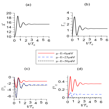
Figure 7: (a) the shifted inter-dot tunnel coupling $\Delta^{\prime}(t)$, (b)-(d) the dissipation-fluctuation matrix elements $\Gamma_{11}(t)$, and $\Gamma^{\beta}_{11,12}(t)$ by varying the chemical potential $\mu=\mu_{L,R}$. The dot parameters $E=E_{1}=E_{2}$ and $\Delta=10~{}\mu$eV. $\Gamma_{L,R}=\Delta$ and $d_{L,R}=\Delta/2$. The matrix $\Gamma^{\beta}$ is hermitian so that only one of the off-diagonal elements is presented here. The red solid, blue long dashed and the black short dashed lines correspond to $\mu-E=0,~{}25$ and 50 $\mu$eV respectively.

Fig. 8 is the same plot with varying the electron tunneling rates between the reservoirs and dots but fixing the chemical potentials at $\mu-E=\Delta$. The small tunneling rate $\Gamma_{L,R}=2.5~{}\mu$eV ($\leq\Delta/2$) does not show a significant time variation in the dissipation-fluctuation coefficients, as also shown in Fig. 4. The shifted inter-dot tunnel coupling at this tunneling rate is very close to the bare one ( $\sim\Delta$), see the red solid line in Fig. 8(a). This implies that a small electron tunneling rate between the reservoirs and dots (corresponds to a small leakage effect) does not manifest the non-Markovian dynamics significantly. Increasing the tunneling rates enlarges the charge leakage effect from the reservoirs to dots and vice versa, thus enhances the non-Markovian effects as well, as shown by the giggling and wiggling time evolutions of the dissipation-fluctuation coefficients in the figure. The time-dependence of shifted inter-dot tunnel coupling $\Delta^{\prime}$ at large tunneling rates also has a significant shift from the bare one $\Delta$ besides the oscillation within the non-Markovian time region. Meanwhile, the charge oscillation frequency has different shifts from the bare Rabi frequency for different $\Gamma_{L,R}$ values. How these time-dependent (non-Markovian) behaviors influent the charge coherence will be discussed in details in the next subsection.

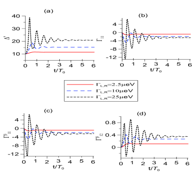
Figure 8: The same plot as in Fig. 7 with fixing the chemical potentials at $\mu-E=\Delta$ and varying the electron tunneling rates between the reservoirs and dots $\Gamma_{L,R}$ symmetrically. The other parameters are the same as in Fig. 7.

Fig. 9 shows how the time-dependence of the shifted inter-dot tunnel coupling and the dissipation-fluctuation coefficients change by varying the spectral widths $d_{L,R}$. We plot these time-dependent coefficients for three different spectral widths: $d_{L,R}$ = 1, 5 and 25 $\mu$eV. The result shows that when $d_{L,R}=25~{}\mu$eV, the dynamics of the double dot already reaches to the Markovian limit, namely all the time-dependent coefficients approach to their asymptotic values in a very short time (less than a half cycle of the bare Rabi oscillation). When the spectral widths $d_{L,R}$ becomes small ($\leq\Delta$) so that the characteristic time of the reservoirs becomes long), the time oscillation of all the transport coefficients becomes strong. Correspondingly the charge dynamics is dominated by non-Markovian processes.

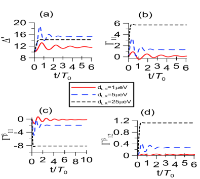
Figure 9: The same plot as in Fig. 8 by varying $d_{L,R}$ but fixing $\Gamma_{L,R}=\Delta$ and other parameters are those used in Fig. 8.

The above numerical results tell that the spectral widths $d_{L,R}$ of the reservoirs (mainly as a memory effect) and the tunneling rates $\Gamma_{L,R}$ between the reservoirs and dots (mainly as a leakage effect) are two basic parameters to characterize the occurrence of non-Markovian dynamics in this double dot device. Comparing the results of Figs. 7, 8 and 9, we find that for the coherence manipulation of charge qubit where the the double dot is unbiased hayashi , the time for the dissipation-fluctuation coefficients reaching to a steady limit depends on the spectral widths of the tunneling spectra as well as the tunneling rates between the reservoirs and dots. The Markovian limit often used in the literature is valid for the electron reservoirs having a relatively small tunneling rate (negligible leakage effect) and a large spectral width (negligible memory effect). The former implies the validity of the Born approximation and the latter corresponds to the Markovian approximation. The chemical potentials of the electron reservoirs controled by the external bias voltage just modifies the values of the dissipation-fluctuation coefficients $\Gamma^{\beta}$ without altering the characteristic times of the reservoirs and the system, as shown in Figs. 3 and 7. However, the chemical potential can be very efficient to suppress the leakage effect. Thus, $\mu-E$ is a competitive control parameter in the coherence control of charge qubit, as we will see later.

In order to show clearly when non-Markovian or Markovian processes play a major role in charge qubit decoherence, we take $\Gamma_{11}$ as an example to examine at what time this dissipation-fluctuation coefficient reaches its steady value by varying $d_{L,R}$ and $\Gamma_{L,R}$. The result is plotted in Fig. 10. The lines signify transition times between the time-dependent fluctuating and the steady dissipation-fluctuation coefficients by varying tunneling rate at a given spectral width. Non-Markovian dynamics can be seen mostly in the time range under the lines. It shows that the strong non-Markovian dynamics corresponds to a relatively small spectral widths $d_{L,R}$ (a strong memory effect) and a relatively large tunneling rates $\Gamma_{L,R}$ (a large leakage effect) compared with the inter-dot tunnel coupling $\Delta$. Non-Markovian dynamics disappears for a large $d_{L,R}$ ($\geq 2\Delta$) and a small $\Gamma_{L,R}$ ($\leq\Delta/2$). In the parameter range of interests to the experimentsprs , the non-Markovian processes do not go over more than five Rabi cycles, with which a significant effect can be seen in maintaining charge coherence, as we will see below.

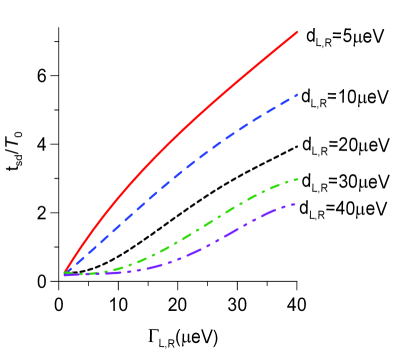
Figure 10: The lines to separate the Markovian and the non-Markovian dynamics in the $\Gamma_{11}-t$ plot, each line corresponds to a given value of $d_{L,R}$. The parameters $\mu-E=\Delta=10\mu$eV are used.

IV.2 Decoherence dynamics of charge qubit

Have examined the time dependencies of all the transport coefficients (the shifted energy level splitting $\varepsilon^{\prime}(t)$, the renormalized inter-dot tunnel coupling $\Delta^{\prime}(t)$ and the dissipation-fluctuation coefficients $\Gamma(t),\Gamma^{\beta}(t)$) in the master equation for both biased and unbiased double dot, we shall discuss now the decoherent dynamics of the charge qubit in this subsection. Experimentally the coherence manipulation of charge qubit is performed for the double dot on resonance, $\varepsilon=E_{1}-E_{2}=0$. The corresponding shifted energy level splitting $\varepsilon^{\prime}(t)$ remains zero. Then the energy eigenbasis of the charge qubit refers actually to the molecular anti-bonding and bonding states, namely, $|\pm\rangle\equiv{1\over\sqrt{2}}(|1\rangle\pm|2\rangle)$. The oscillation between the coherently coupled localized charge states $|1\rangle$ and $|2\rangle$ as coherent superpositions of the molecular states describes the charge coherence, where the renormalized Rabi frequency $\Omega(t)=\Delta^{\prime}(t)$ is just the shifted inter-dot tunnel coupling for the symmetric double dot. The time-dependent dissipation-fluctuation coefficients $\Gamma(t),\Gamma^{\beta}(t)$ will disturb this coherent oscillation and cause charge qubit decoherence.

To be specific, we let the initial state be $\rho_{11}=1$ and examine the time evolution of the density matrix under various conditions. We calculate first the rate equations (38) for the no-Coulomb-interacting double dot. The typical population evolution shown in Fig. 11 tells that the double occupancy is favored. In fact, the charge qubit of a double dot is designed in the strong inter-dot Coulomb blockade regime where the state of simultaneous occupation of two dots is excluded. In other words, unlike the charge qubit initialization where both the interaction-free and the strong interaction rate equations give qualitatively the same result, for the coherence control of the charge qubit the interaction-free rate equations (38) is invalid. The charge qubit dynamics must be described by the strong-interaction rate equations (47).

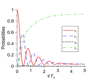
Figure 11: The time evolutions of the populations $\rho_{11}$(the red solid line), $\rho_{22}$(the blue long-dashed line), $\rho_{00}$(the black short dashed line), and $\rho_{33}$(the green dashed-dotted line) calculated using the interaction-free rate equations (38) in the symmetric double dot with $\Delta=10\mu$eV, $\mu-E=30\mu$eV, $d_{L,R}=\Delta/2$ and $\Gamma_{L,R}=d_{L,R}$. Without considering the inter-dot Coulomb repulsion, raising up of the chemical potentials $\mu>E$ accumulates charges into the double dot.

For the rate equations (47) in the strong inter-dot Coulomb repulsion regime to be held for charge qubit manipulation, the energy difference between the fermi surfaces of the reservoirs and the energy levels of the dots, $\mu-E$, cannot be too large. The inter-dot Coulomb repulsion in the samples is estimated to be 200$\mu$eV hayashi . The value of $\mu-E$ that can be taken most safely should be not larger than $50\mu$eV, a quarter of the inter-dot Coulomb repulsion energy. If $\mu-E$ is taken over 100 $\mu$eV, it is comparable to the Coulomb repulsion energy so that the doubly occupied state cannot be completely excluded. For convenience and consistency with the discussion in the previous subsection, we still take the quantum dot parameters $E_{1}=E_{2}=E$ and $\Delta=10\mu$eV. As one will see with $\mu-E=25\sim 50\mu$eV, and $\Gamma_{L,R}$ and $d_{L,R}$ being in a reasonable range, the charge qubit can maintain coherence very well.

In Fig. 12, we plot the time evolution of the reduced density matrix by varying the aligned fermi surfaces. The result shows that the coherent oscillation of the charge qubit depends sensitively on the hight of aligned fermi surfaces from the resonant levels of the double dot, i.e., $\mu-E$. When $\mu-E$ is not too large ($<\Delta$) and $\Gamma_{L,R}$ is not too small ($>\Delta$), the population $\rho_{11}$ decays very quickly. This is because although the state of simultaneous occupation of two dots is excluded, there is still chance for electrons to escape from the dots into the reservoirs such that both dots become empty, namely $\rho_{00}\neq 0$ [see Fig. 12(b)] as a leakage effect. This effect can be suppressed when the fermi surfaces are aligned such that $\mu-E$ must be relatively larger than $\Gamma_{L,R}$. As a result, the charge qubit can maintain the coherence very well. In Fig. 12(a), we see that the charge coherence is perfectly maintained for $\mu-E=50\mu$eV. Meanwhile, the real part and the imaginary part of the off-diagonal density matrix element $\rho_{12}$ exhibit quite different dynamics. The imaginary part of $\rho_{12}$ has a similar oscillatory feature as $\rho_{11}$ [see Fig. 12(d)], which depicts the coherent tunnel coupling between two dots. While the real part of $\rho_{12}$ goes down to be negative [see Fig. 12(c)] which is related to the loss of the energy (dissipation). We find that to maintain a good coherent dynamics for charge qubit, the fermi surfaces of the reservoirs is better to be aligned above the energy levels of the double dot not less than $2\Delta$.

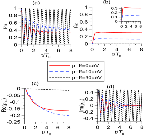
Figure 12: The time evolutions of the density matrix at different $\mu-E$ with $E$ fixed. The red solid line is for $\mu-E=0$, the blue long-dashed line is for $\mu-E=10\mu$eV and the black short-dashed line is for $\mu-E=50\mu$eV. $d_{L,R}=\Delta/2$ and $\Gamma_{L,R}=\Delta$.

In Fig. 13 we plot the time evolution of the reduced density matrix at a few different tunneling rates but fixing other parameters. Experimentally, the tunneling rates between the dots and the reservoirs are also tunable. We fixed the spectral widthes at $d_{L,R}=25\mu$eV for which the memory effect is largely suppressed. Meantime, we take $\mu-E=50\mu$eV (much larger than $\Gamma_{L,R}$) such that the leakage effect is also largely suppressed. When the tunneling rates are small ($<\Delta/2$), the time-dependence of these transport coefficients in the master equation are negligible (as shown in Fig. 8) so that no non-Markovian dynamics can be observed. The corresponding charge dynamics is given by the red solid lines in Fig. 13 where the oscillation frequency is time independence, consistent with the result in Markovian approximation. When the tunneling rates become large ($\geq\Delta$), the charge frequency is largely shifted and varies in time. The larger the tunneling rates are, the faster the electron oscillates between two dots and the reservoirs, thus the stronger the non-Markovian dynamics occurs. Here the decay of the coherent charge oscillation (see the blue long-dashed and black short-dashed lines in Fig. 13) is not due to the charge leakage (which has been mainly suppressed by raising up the fermi surfaces) but a back-action decoherence effect of the reservoirs when the tunneling rate becomes larger. Increasing the tunneling rates leads to more charge leakage. However, comparing the magnitude of $\rho_{00}$ with that of $\rho_{11}$ shows that the damping of coherent charge oscillation in the presence of a large tunneling rate is not primarily due to charge leakage but a non-Markovian back-action decoherence effect.

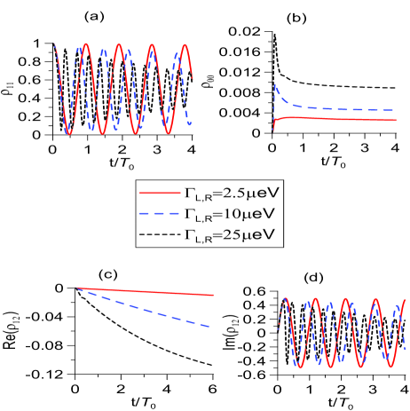
Figure 13: The time evolutions of the density matrix at different coupling constants. The red solid line is for $\Gamma_{L,R}=2.5\mu$eV, the blue long-dashed line is for $\Gamma_{L,R}=10\mu$eV and the black short-dashed line is for $\Gamma_{L,R}=25\mu$eV. The chemical potentials are kept at $\mu-E=50\mu$eV and $d_{L,R}=25\mu$eV.

The more non-Markovian dynamics can be seen by varying the spectral widths $d_{L,R}$. When the spectral width is comparable to the inter-dot coupling $\Delta$, namely the characteristic time of reservoirs is comparable to the characteristic time of the double dot, the non-Markovian dynamics becomes the most significant in the time evolution of charge coherence. Although it is currently not clear how to tune the spectral widths in experiments, it is still interesting to see what roles the spectral widths (or more generally speaking, a non-constant spectral density) play in the charge decoherence dynamics. We plot in Fig. 14 the time evolutions of the density matrix elements at various spectral widths with $\mu-E=50\mu$eV and $\Gamma_{L,R}=\Delta$. As we can see if $d_{L,R}$ is small ($\leq\Delta/2$), the coherent charge dynamics is well preserved although it is a strong non-Markovian process. With increasing the spectral widths, the decoherent charge dynamics becomes visible and also becomes Markov type. Widening the spectral widthes damps the coherent charge oscillation. Wider spectral width also causes more charge leakage. But comparing the magnitudes of $\rho_{00}$ with $\rho_{11}$ in Fig. 14 shows again that the damping of coherent charge oscillation in the presence of a wide spectral width is a Markovian back-action decoherence effect. The frequencies of coherent charge oscillation are also shifted differently from the bare Rabi frequency for different spectral widths presented. [see Fig. 14(a)-(d)].

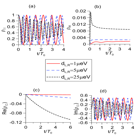
Figure 14: The time evolutions of the density matrix at different spectral widths. The red solid line is for $d_{L,R}=1\mu$eV, the blue long-dashed line is for $d_{L,R}=5\mu$eV and the black short-dashed line is for $d_{L,R}=25\mu$eV. $\mu-E$ is kept at $50\mu$eV and $\Gamma_{L,R}=\Delta$.

From the above analysis, we find that the charge qubit coherence can be maintained very well when either the spectral widths $d_{L,R}$ or the tunneling rates $\Gamma_{L,R}$ are sufficiently smaller than $\mu-E$. However, when both the spectral widths $d_{L,R}$ and the tunneling rates $\Gamma_{L,R}$ become comparable to $\mu-E$, the decay of charge coherency can be seen within a few cycles of the bare Rabi oscillation. The difference between the non-Markovian and the Markovian process manifests in the difference between the renormalized Rabi frequency $\Omega(t)=\Delta^{\prime}(t)$ (for the symmetric double dot) and the bare Rabi frequency $\Omega_{0}=\Delta$. In Fig. 15, we plot the average renormalized Rabi freuency $\langle\Omega\rangle=\overline{\Omega(t)}$ by varying the spectral widths $d_{L,R}$ and the tunneling rate $\Gamma_{L,R}$, respectively, and make a comparison with the bare Rabi frequency (the black short dashed lines). It shows that the renormalized Rabi frequency has a large shift from the bare one, except for the region (the Markovian regime) with the spectral width $d_{L,R}>2\Delta$ and the tunneling rate $\Gamma_{L,R}<\Delta/2$, where the renormalized Rabi frequency is close to the bare one. In Fig. 16, we plot the time evolution of density matrix $\rho_{11}$ using the strong-interaction rate equations (47) for a few different sets of ($\Gamma_{L,R},d_{L,R}$) and make a comparison with the Markovian approximation determined by the rate equations (48), where the charge coherence dynamics in the double dot from Markovian to the non-Markovian processes is clearly demonstrated.

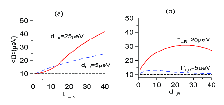
Figure 15: The average renormalized Rabi frequency $\langle\Omega\rangle=\overline{\Omega(t)}$ by varying the spectral widths $d_{L,R}$ and the tunneling rate $\Gamma_{L,R}$, respectively, and comparing with the bare Rabi frequency (the black short dashed lines). Here we take $\mu-E=50\mu$eV to suppress the charge leakage.

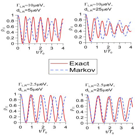
Figure 16: The time evolutions of $\rho_{11}$ obtained from the rate equation (47) and the corresponding Markovian limit (48) for the strong-Coulomb-interacting double dot. (a) the strongest non-Markovian regime for a small spectral width and a large tunneling rate. (b) the non-Markovian dynamics controlled by a large tunneling rate alone. (c) the non-Markovian dynamics controlled by a small spectral width alone. (d) The Markovian regime corresponding to a small tunneling rate and large spectral width. Here we take $\mu-E=30\mu$eV.

IV.3 Relaxation time $T_{1}$ and dephasing time $T_{2}$

To understand quantitatively the decoherence dynamics of charge qubit in the double dot, we shall now extract the decay rates (the relaxation time $T_{1}$ and the dephasing time $T_{2}$) for various manipulation conditions. The relaxation time $T_{1}$ characterizes the time going from the anti-bonding state (with higher energy) to the bonding state (with lower energy) in the energy eigenbasis $|\pm\rangle={1\over\sqrt{2}}(|1\rangle\pm|2\rangle)$ (for symmetric double dot). It is described by the decay of the diagonal element of the density matrix in the energy eigenbasis, $\langle+|\rho|+\rangle={1\over 2}(\rho_{11}+\rho_{22})+\mbox{Re}(\rho_{12})$. In the ideal case (such as in NMR), $\rho_{11}+\rho_{22}=1$ so that $T_{1}$ is completely determined by the real part of $\rho_{12}$. For the charge qubit in double dots, in general $\rho_{11}+\rho_{22}<1$ because of charge leakage. But in the practical manipulation, the fermi surfaces of the reservoirs are set high enough from the resonant energy levels of the double dot such that charge leakage can be suppressed. Thus we can still extract $T_{1}$ from $\mbox{Re}\rho_{12}$. The decoherence (dephasing) time $T_{2}$ corresponds to the decay of the off-diagonal element of the reduced density matrix $\langle+|\rho|-\rangle={1\over 2}(\rho_{11}-\rho_{22})-i\mbox{Im}(\rho_{12})$. As we will see later the time-dependencies of $\rho_{11},\rho_{22}$ and the imaginary part of $\rho_{12}$ behave very similar. This may tell us that $T_{2}$ can be extracted either from $\rho_{11},\rho_{22}$ or $\mbox{Im}\rho_{12}$. Experimentally, one extracted $T_{2}$ from $\rho_{22}$ by measuring the current proportion to $\rho_{22}$ hayashi .

Having made the above analysis, we shall extract the decay rates of the charge coherent oscillations from the time evolution of the reduced density matrix elements $\mbox{Re}\rho_{12}(t)$ and $\mbox{Im}\rho_{12}(t)$ or $\rho_{11}(t)$ by fitting a decay oscillating function plus an offset to the numerical data. An intuitive fitting function for the charge oscillation decay would be $Ae^{-Bt}\cos(\langle\Omega\rangle t)+C$. However this fitting function fails for $\rho_{11}(t)$. The typical damping oscillation of $\rho_{11}(t)$ shows that it converges to a steady value of $\rho_{11}\leq{1\over 2}$ at large $t$. Thus $\rho_{11}(t)$ can be well described by the fitting function

$$\rho_{11}(t)=f_{h}(t)\cos^{2}(\langle\Omega\rangle t/2)+f_{l}(t)\sin^{2}(\langle\Omega\rangle t/2)$$ (52)

where $f_{h,l}(t)=A_{h,l}\exp(-B_{h,l}t^{s})+C_{h,l}$ are used to fit the downward shift of the peaks and the upward shift of the valleys in the damped oscillation, respectively. The oscillating function is the squares of sine and cosine functions with half the oscillation frequency, $\sin^{2}(\langle\Omega\rangle t/2)$ and $\cos^{2}(\langle\Omega\rangle t/2)$, rather than $\cos(\langle\Omega\rangle t)$ and $\sin(\langle\Omega\rangle t)$. This can be easily understood by considering an ideal qubit. Its Rabi oscillation conditioned to the initial state $\rho_{11}(0)=1$ is given by $\rho(t)=\begin{pmatrix}\cos^{2}(\Omega t/2)&-{i\over 2}\sin(\Omega t)\\ {i\over 2}\sin(\Omega t)&\sin^{2}(\Omega t/2)\end{pmatrix}$ in the localized charge state basis. Similarly, the off-diagonal density matrix elements can be described by the fitting functions

$$\mbox{Im}\rho_{12}(t)=\big{\{}A_{i}\exp(-B_{i}t^{s})+C_{i}\big{\}}\sin(\langle\Omega\rangle t),$$ (53a)

$$\mbox{Re}\rho_{12}(t)=A_{r}\exp(-B_{r}t^{s})+C_{r}.$$ (53b)

The fitting parameters $A_{x},B_{x},C_{x}$ for $x=h,l,i,r$ are generally different for different fitting function and different data. Fig. 17 is a plot of using the fitting function of (52) to fit the exact numerical solution of $\rho_{11}(t)$. The results show that with the decay function $f_{h}(t)=0.48\exp{(-0.58t)}+0.50$ and $f_{l}(t)=-0.47\exp(-0.54t)+0.49$, the fitting function (52) gives very much the same solution as that obtained numerically from Eq. (47) for $\rho_{11}(t)$.

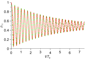
Figure 17: (a) Using the fitting function $f_{h}(t)\cos^{2}(\langle\Omega\rangle t/2)+f_{l}(t)\sin^{2}(\langle\Omega\rangle t/2)$ (the red solid line) to fit the exact numerical solution of $\rho_{11}(t)$ (the green dashed-dotted line). Here we use the parameters $\mu-E=50\mu$eV, $\Gamma_{L,R}=25\mu$eV and $d_{L,R}=25\mu$eV.

In order to have a better fitting to various tunable parameters, we plot in Fig. 18 the fitting errors for $\rho_{11}(t)$ by averaging the deviations between $f_{h}(t)$ and the peaks of the oscillating $\rho_{11}(t)$ in a large range of the chemical potential, the tunneling rate as well as the spectral width. The top two plots in Figs. 18 are the fitting errors by varying $\mu_{L,R}$ but fixing $(\Gamma_{L,R},d_{L,R})=(25,5)\mu$eV (the strong non-Markovian regime) and (5, 25) $\mu$eV (the Markovian limit regime). We find that in the strong non-Markovian regime, when the fermi surfaces are not far away from the resonant levels of the double dot ($\mu-E<25\mu$eV), the best fitting is a sub-exponential decay with $s<1$. When $\mu-E>25\mu$eV, the fitting function becomes a simple exponential decay function ($s=1$), while, in the Markovian limit, the best fitting is just a simple exponential decay for all the values of $\mu-E$. The middle two plots in Figs. 18 are the fitting errors by varying $\Gamma_{L,R}$ but fixing $(\mu-E,d_{L,R})=(10,5)\mu$eV (the non-Markovian regime) and (30, 25) $\mu$eV (the Markovian limit). Again we see that in the non-Markovian regime, the best fitting is a sub-exponential decay with $s<1$ for all the values of $\Gamma_{L,R}$ except for some very small $\Gamma_{L,R}$ ($<\Delta/2$) which indeed enters the Markovian limit where the fitting function becomes a simple exponential decay function. In the Markovian limit (the large spectral width limit here), the best fitting is given by a simple exponential decay ($s=1$) again. The bottom two plots in Figs. 18 are the fitting errors by varying $d_{L,R}$ but fixed $(\mu-E,\Gamma_{L,R})=(10,25)\mu$eV (the non-Markovian regime) and (30, 5) $\mu$eV (the Markovian limit). It tells that in the non-Markovian regime, when $d_{L,R}<\Delta$ (the strong non-Markovian regime), the best fitting is still given by a sub-exponential decay ($s<1$), while for $d_{L,R}>\Delta$ the system transits to the Markovian, the fitting function becomes again a simple exponential decay function. In the Markovian limit (small tunneling rate limit), the best fitting is just given by a simple exponential decay ($s=1$), as one expected.

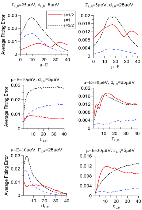
Figure 18: The average fitting errors by fitting the exact numerical solutions of $\rho_{11}(t)$ with the fitting function given by Eq. (52). The top two plots are the fitting errors by varying $\mu-E$ but fixing $(\Gamma_{L,R},d_{L,R})=(25,5)\mu$eV and (5, 25) $\mu$eV, respectively; The middle two plots for varying $\Gamma_{L,R}$ but fixing $(\mu-E,d_{L,R})=(10,5)\mu$eV and (30, 25) $\mu$eV; and the bottom two plots are obtained by varying $d_{L,R}$ but fixed $(\mu-E,\Gamma_{L,R})=(10,25)\mu$eV and (30, 5) $\mu$eV. The parameters are chosen such that the left three figures correspond to the non-Markovian regime while the right three figures are the Markovian limit. $s=1/2$ corresponds to the sub-exponential fitting (red lines), $s=1$ is the simple exponential fitting (blue long-dashed lines), and $s=3/2$ is the super-exponential fitting (black dashed lines).

The above analysis shows that Markovian decoherence processes lead to an exponential decay and a sub-exponential decay seems to occur mainly in strong non-Markovian processes. But this does not imply a simple exponential decay being necessarily Markovian. In Fig. (19), we plot the average fitting errors of the fitting functions (53) with the exact numerical solution of the real and imaginary parts of the off-diagonal density matrix element $\rho_{12}(t)$ in the strong non-Markovian regime with the spectral widths $d_{L,R}=5\mu$eV and the tunneling rates $\Gamma_{L,R}=25\mu$eV. The results show that for both $\mbox{Im}\rho_{12}(t)$ and $\mbox{Re}\rho_{12}(t)$, the best fitting is given by simple exponential decay for the whole range of chemical potential up to $\mu-E=40\mu$eV. This forces us to carefully look at the results in Fig. 18. We find that all the results with a sub-exponential decay show up for small $\mu-E$ values ($<2\Delta$) where the charge leakage effect cannot be effectively suppressed by the chemical potentials of the reservoirs. This tells that the sub-exponential decay in $\rho_{11}(t)$ is a charge leakage effect. The slightly different decay behaviors for $\rho_{11}(t)$ and $\mbox{Im}\rho_{12}(t)$ actually come from the charge leakage effect contained in $\rho_{11}(t)$ rather than a consequence of non-Markovian dynamics, as we will see more later.

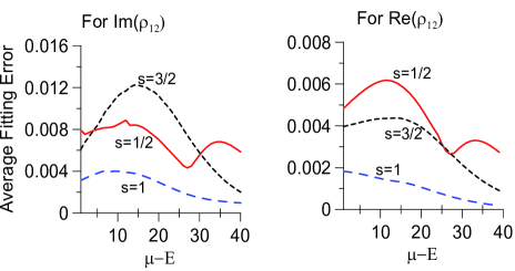
Figure 19: The average fitting errors by fitting the exact numerical solution of $\mbox{Im}\rho_{12}(t)$ and $\mbox{Re}\rho_{12}(t)$ with the fitting functions given by Eq. (53), where we vary $\mu-E$ but fixing $d_{L,R}=5\mu$eV and $\Gamma_{L,R}=25\mu$eV. The red lines correspond to the sub-exponential fitting function ($s=1/2$), the blue long-dashed lines are the simple exponential fitting function ($s=1$), and the black dashed lines are the super-exponential fitting function ($s=3/2$).

Now we shall extract the relaxation time $T_{1}$ from $\mbox{Re}\rho_{12}(t)$ and the decoherence time $T_{2}$ from $\mbox{Im}\rho_{12}(t)$ or $\rho_{11}(t)$ using the concept of half life from the exact numerical solutions and from the fitting functions (53) and (52). The results is plotted in the Figs. 20-22. In Fig. 20 we plot the relaxation time $T_{1}$ and the decoherence time $T_{2}$ from $\mbox{Re}\rho_{12}(t)$ and $\mbox{Im}\rho_{12}(t)$, respectively, by varying the chemical potential $\mu-E$, the tunneling rates $\Gamma_{L,R}$ and the spectral widths $d_{L,R}$ differently. Fig. 20(a)-(b) are the plots of $T_{1}$ and $T_{2}$ by varying $\mu-E$ but fixing $(\Gamma_{L,R},d_{L,R})=(25,5)\mu$eV (solid lines, corresponding to the non-Markovian processes) and (5, 25) $\mu$eV (dashed lines for Markovian limit). The results tell that the decoherence effect (for both $T_{1}$ and $T_{2}$) is large for the small chemical potential $\mu-E$ due to the large charge leakage effect. Increasing $\mu-E$ reduces the charge leakage effect, thus also reduces the decoherence effect. When $\mu-E$ is larger than $\Gamma_{L,R}$ and $d_{L,R}$ [goes up to 30 $\mu$eV in Fig. 20(a)-(b)], the decoherence effect quickly reaches to a minimum value (the longest decoherence time $\sim$ 2 ns). Fig. 20(c)-(d) plot $T_{1}$ and $T_{2}$ by varying $\Gamma_{L,R}$ but fixing $(\mu-E,d_{L,R})=(10,5)$ (solid lines, where both the charge leakage effect and the memory effect are supposed to play an important role) and (30, 25) $\mu$eV (dashed lines, where both the charge leakage effect and the memory effect are ignorable). It shows that for a small tunneling rate between the reservoir and dot ($<\Delta$) the decoherence effect is weak. Increasing $\Gamma_{L,R}$ enhances the non-Markovian dynamics effect and also enhances the decoherence (shorting the relaxation and dephasing times). Fig. 20(e)-(f) plot $T_{1}$ and $T_{2}$ by varying $d_{L,R}$ but fixing $(\mu-E,\Gamma_{L,R})=(10,25)$ (solid lines, where the charge leakage effect is dominated) and (30, 5) $\mu$eV (dashed lines, where the charge leakage effect is negligible). We find that when the memory effect must be considered (corresponding to a small spectral width), the decoherence effect is small (or the relaxation and dephasing times become longer). Increasing $d_{L,R}$ reduces the memory or non-Markovian dynamics effect and enhances the decoherence (shorting the relaxation and dephasing times). It is interesting to see that in all the cases, the relaxation time is close to the dephsing time: $T_{1}\simeq T_{2}$ in the Markovian limit (dashed lines), where for the non-Markovian regime, the relaxation time is larger than the dephasing time up to twice: $T_{1}\leq 2T_{2}$ (solid lines).

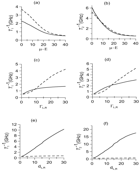
Figure 20: The relaxation time $T_{1}$ and the dephasing time $T_{2}$ extracted from $\mbox{Re}\rho_{12}(t)$ and $\mbox{Im}\rho_{12}(t)$, respectively, (a)-(b) by varying the chemical potential $\mu-E$ but fixing $(\mu-E,d_{L,R})=(10,5)$ (solid lines) and (30, 25) $\mu$eV (dashed lines), (c)-(d) by varying the tunneling rates $\Gamma_{L,R}$ at $(\mu-E,d_{L,R})=(10,5)$ (solid lines) and (30, 25) $\mu$eV (dashed lines), and (e)-(f) by varying the spectral widths $d_{L,R}$ but fixing $(\mu-E,\Gamma_{L,R})=(10,25)$ (solid lines) and (30, 5) $\mu$eV (dashed lines).

As we have pointed out that the decay behaviors for $\rho_{11}$ and $\mbox{Im}\rho_{12}$ are slightly different from the fitting function in the non-Markovian regime. In Fig. 21, we compare the decoherence time $T_{2}$ extracted from $\rho_{11}(t)$ and $\mbox{Im}\rho_{12}(t)$, respectively, with the same conditions as used in Fig. 20, namely by varying the chemical potential $\mu-E$, the tunneling rates $\Gamma_{L,R}$ and the spectral widths $d_{L,R}$ differently. As we see although quantitatively the dephasing time extracted from $\rho_{11}(t)$ and $\mbox{Im}\rho_{12}(t)$ are in the same order, but there are some obvious differences in certain range of the tunable parameters where the charge leakage effect play an important role. This is indeed clearly show in the right-bottom two plots in Fig. 21 where $\mu-E=30\mu$eV. When $\Gamma_{L,R}$ are small ($\leq\Delta/2$) so that the charge leakage is negligible, the dephasing time $T_{2}$ extracted from $\rho_{11}(t)$ and $\mbox{Im}\rho_{12}(t)$ are very close to each other over there. This again indicates that it is the charge leakage effect that results in the slightly different decay law for $\rho_{11}(t)$ (follows a sub-exponential decay) and $\mbox{Im}\rho_{12}(t)$ (by a simple exponential decay) in the non-Markovian regime.

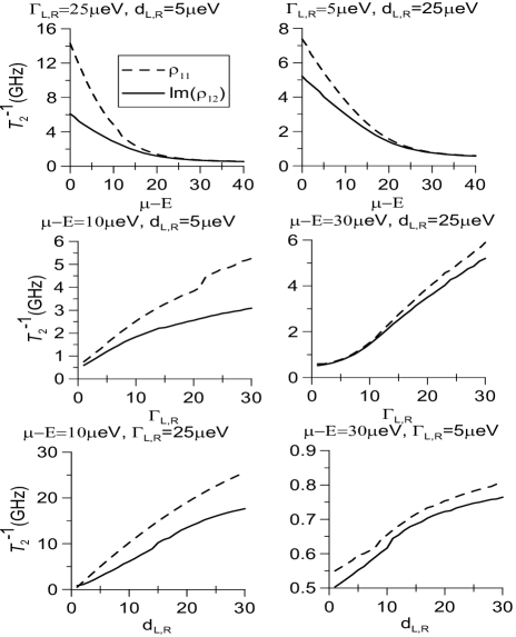
Figure 21: The decoherence time $T_{2}$ extracted from $\rho_{11}(t)$ and $\mbox{Im}\rho_{12}(t)$, respectively, with the same conditions used in Fig. 20, namely by varying the chemical potential $\mu-E$, the tunneling rates $\Gamma_{L,R}$ and the spectral widths $d_{L,R}$ differently.

In fact, the original definition of the decoherence for a qubit is given by the decay of $|\langle+|\rho|-\rangle|$ though it is not easy to be measured directly in experiments. Ultimately when the charge qubit is completely decohered, $\rho_{11}\sim\rho_{22}$ and $\mbox{Im}(\rho_{12})\sim 0$ thus $|\langle+|\rho|-\rangle|\sim 0$ at the asymptotic time. We have verified this property in our exact numerical calculation. Thus the off-diagonal reduced density matrix element in the energy eigenbasis, $|\langle+|\rho(t)|-\rangle|$, can be well fitted by $Ae^{-Bt^{s}}+C$ with $C=0$. In Fig. 22 we compare the results of $T_{2}$ extracted from $|\langle+|\rho|-\rangle|$ and $\mbox{Im}(\rho_{12})(t)$, respectively. It is remarkable that the dephasing time $T_{2}$ obtained from $|\langle+|\rho|-\rangle|$ and $\mbox{Im}(\rho_{12})(t)$ are almost exactly the same in a wide range of parameters concerned here( $\mu-E$ is from 0 to $40\mu$eV, $\Gamma_{L,R}$ and $d_{L,R}$ are from 1 to $30\mu\mbox{eV}$ at $\Delta=10\mu$eV). The decoherence (dephasing) time $T_{2}$ obtained here is between 0.2 to 2 ns, except for the case shown in the left-bottom plot in Fig. 21 where the decoherence time even smaller.

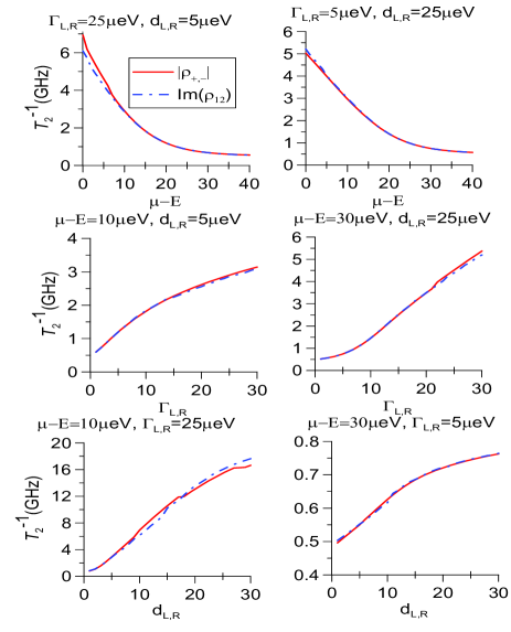
Figure 22: The decoherence time $T_{2}$ extracted from $|\rho_{+,-}(t)|=|\langle+|\rho|-\rangle|$ and $\mbox{Im}\rho_{12}(t)$, respectively, with the same conditions used in Fig. 21, namely by varying the chemical potential $\mu-E$, the tunneling rates $\Gamma_{L,R}$ and the spectral widths $d_{L,R}$ differently.

Now we shall end this section with a brief summary in the following. The non-Markovian coherence and decoherence dynamics of charge qubit is dominated by two major effects, the memory effect and the leakage effect in the double dot gated by electrode reservoirs. The former becomes a dominate effect when the time scale of the reservoirs is comparable to the time scale of the double dot. The latter becomes an important effect when the electron tunneling strength between the reservoirs and dots is tuned to be large. These two characters are suitably described by the spectral widths and the tunneling rates embedded in the Lorentzian spectral density (25) we used. Strengthening the couplings between the reservoirs and dots and widening the spectral widths of the reservoirs disturb the charge coherence in the double dot significantly. However, reasonably raising up the chemical potentials $\mu_{L,R}$ can suppress charge leakage and maintain charge coherence. The left uncontrollable decoherence factor is the spectral width which characters how many electron states in the reservoirs effectively involving in the tunneling processes between the dots and the reservoirs. The smaller the spectral width is (the less the electron states involve in the electron tunneling), the better the charge coherence can be maintained. The decay of the charge coherent oscillation is well described by a simple exponential decay for the off-diagonal reduced density matrix elements, but the diagonal ones (populations) are better described by a sub-exponential law when charge leakage is not negligible. Otherwise simple exponential decay is better for both the non-Markovian and Markovian regimes. The relaxation time $T_{1}$ and the dephasing time $T_{2}$ can be extracted from the exact numerical solution $\mbox{Re}\rho_{12}(t)$ and $\mbox{Im}\rho_{12}(t)$, respectively, with the result $T_{1}\leq 2T_{2}$ for a broad parameter range we used.

V Conclusion and Discussion

In this paper, we have developed a non-perturbation theory to describe decoherence dynamics of electron charges in the double quantum dot gated by electrodes. We extended the Feynman-Vernon influence functional theory to fermionic environments and derived an exact master equation (33) for the reduced density matrix of the double dot without including the inter-dot Coulomb repulsion at beginning. The contributions of quantum and thermal fluctuations induced by the electron reservoirs are embedded into the time-dependent transport coefficients (34) and (37) in the master equation. These time-dependent transport coefficients are completely determined by the non-perturbation dissipation-fluctuation equations of motion (30). The exact master equation is then further extended to the double dot in the strong inter-dot Coulomb interacting regime in terms of Bloch-type rate equations (47) where the strong Coulomb repulsion simply leads one to exclude the states corresponding to a simultaneous occupation of the two dots from Eq. (33). Our theory is developed for a general spectral density of the reservoirs at arbitrary temperatures and bias. Other approximated master equations used for the double quantum dot can be obtained at well defined limits of the present theory. This non-perturbation decoherence theory allows us to exploit the quantum decoherence dynamics of the charge qubit brought up by the tunneling processes between the reservoirs and dots through qubit manipulations.

We then used the master equation (in terms of the rate equations) to study the non-Markovian decoherence dynamics of the double dot charge qubit with the back-action of the reservoirs being fully taken into account. To make qualitative and also quantitative understandings of the charge qubit decoherence, we numerically solve the dissipation-fluctuation integro-differential equations of motion using a Lorentzian spectral density. We examine the time dependence of all the transport coefficients from which the time scales within which non-Markovian processes become important in the charge coherent dynamics are determined. The correlation time of the electron reservoirs (in terms of the spectral widths in the Lorentzian spectral densities) and the electron tunneling strengths between the reservoirs and dots (in terms of the tunneling rates in the Lorentzian spectral densities) characterize the time scales for the occurrence of non-Markovian processes. Non-Markovian processes dominate the charge coherent dynamics when the spectral width is comparable to the inter-dot tunnel coupling where the memory effect plays an important role, and/or when the tunneling rates between the reservoirs and dots become strong such that charge leakage becomes a main effect for decoherence. Raising up the fermi surfaces of the reservoirs can suppress charge leakage. The Markovian limit can be reached with a weak tunneling rate and a large spectral width, where perturbation theory becomes valid and the spectral density is reduced to a constant. The decay of the charge coherent oscillation is well described by a simple exponential law, except for some special regime where the charge leakage is not negligible such that the evolution of state populations is better described by a sub-exponential decay. We also extracted the relaxation time $T_{1}$ and the decoherence time $T_{2}$ consistently from different elements of the reduced density matrix and obtained a general result $T_{1}\leq 2T_{2}$ which is of the order of ns or less in a broad parameter range we considered. These results are ready to be examined in experiments prs .

Although we concentrate in this paper the electron charge coherence (decoherence) dynamics in the double quantum dot system, the theory we developed in this work can also be applied to investigate other physical properties, such as quantum transport phenomena, in various quantum dot structures. In fact, the spectral density describing the spectral distribution of electron reservoirs and electron tunneling processes between the reservoirs and dots has not been well determined experimentally. We used a Lorentzian spectral density that has been used by others yet still been waiting for justifying in experiments. The tunneling rates $\Gamma_{L,R}$ in the Lorentzian spectral density is indeed tunable in experiment, and have been extracted from current spectra by assuming a constant spectral density. With the capability of monitoring the time evolution of electronic population transfer, we can look at closely the short time transport properties in this double dot device from which we may extract the tunneling rates and the spectral widths for the Lorentzian spectral density or other possible forms of the spectral density. Otherwise it may be other surroundings (phonons and fluctuation in impurity configurations, etc.) that play an important role in the dynamics of charge qubit decoherence. These together with other transport properties in various nanostructures, such as Kondo effect and Fano resonance, etc., deserve a separate study. We will leave these research problems to be addressed in separate papers.

Appendix A Derivation of the influence functional

The propagating function governing the time evolution of the reduced density matrix is given by Eq. (22), in which the generalized Feynman-Vernon’s influence functional is defined by

$$\mathcal{F}[\xi^{*},\xi,\eta^{*},\eta]= \int d\mu(f_{N})d\mu(f_{0})d\mu(g_{0})\langle f_{0}|\rho_{E}(t_{0})|g_{0}\rangle$$

$$\times\int\mathcal{D}[f^{*},f,g^{*},g]e^{i\big{\{}S_{E}[f^{*},f]-S^{*}_{E}[g^{*},g]}$$

$$~{}~{}~{}~{}~{}~{}~{}~{}~{}~{}^{+S_{I}[\xi^{*},\xi,f^{*},f]-S^{*}_{I}[\eta^{*},\eta,g^{*},g]\big{\}}},$$ (54)

where $\rho_{E}$ is the initial density operator of the fermion reservoirs, $f_{0},g_{0},f_{N}$ and their complex conjugates are Grassmann numbers introduced in the fermion coherent state representation, $S_{E}$ is the action of the electron reservoirs, and $S_{I}$ stands for the action of the interaction between the dots and the reservoirs. Explicitly,

$$iS_{E} [f^{*},f]=\sum_{l=1,2;k}\Big{\{}{f^{*}_{lk}(t)f_{lk}(t)+f^{*}_{lk}(t_{0})f_{lk}(t_{0})\over 2}$$

$$+\int_{t_{0}}^{t}d\tau\Big{[}\Big{(}{\dot{f}^{*}_{lk}f_{lk}-f^{*}_{lk}\dot{f}_{lk}\over 2}\Big{)}-i\varepsilon_{lk}f^{*}_{lk}f_{lk}\Big{]}\Big{\}}$$

$$~{}~{}~{}~{}~{}~{}~{}~{}=i\sum_{lk}S_{E,lk}[f^{*}_{lk},f_{lk}],$$ (55a)

$$S_{I}[\xi^{*}, \xi,f^{*},f]=-\sum_{lk}\int_{t_{0}}^{t}d\tau(t_{ilk}\xi^{*}_{i}f_{lk}+t^{*}_{ilk}f^{*}_{lk}\xi_{i})$$

$$~{}~{}~{}~{}~{}~{}~{}~{}~{}~{}=\sum_{lk}S_{I,lk}[\xi^{*}_{i},\xi_{i},f_{lk}^{*},f_{lk}].$$ (55b)

Let the electron reservoirs be initially in a thermal equilibrium state, then

$$\langle f_{0}|\rho_{E}(t_{0})|g_{0}\rangle=\prod_{lk}\langle f_{k0}|{1\over Z}e^{-\beta(\varepsilon_{lk}-\mu_{l})a^{{\dagger}}_{lk}a_{lk}}|g_{k0}\rangle$$ (56)

where $\mu_{L,R}$ are the chemical potentials of the source and drain electron reservoirs connected to the dots $1$ and $2$, respectively, and $Z$ is the fermion partition function of the reservoirs $Z=\prod_{lk}(e^{-\beta(\varepsilon_{lk}-\mu_{l})}+1)$. Obviously, the influence functional can be written as $\mathcal{F}[\xi^{*},\xi,\eta^{*},\eta]=\prod_{lk}\mathcal{F}_{lk}[\xi^{*},\xi,\eta^{*},\eta]$. Furthermore, since the Hamiltonians are quadratic, the path integrals in the influence functional can be exactly calculated using either the Gaussian integrals or the stationary path method. Here we present the clculation based the stationary path method. The forward stationary pathes of the electrons in the reservoirs is determined by

$$\dot{f}_{lk}(\tau)+i\varepsilon_{lk}f_{lk}(\tau)=-it^{*}_{ilk}\xi_{i}(\tau),~{}$$ (57a)

$$\dot{f}_{lk}^{*}(\tau)-i\varepsilon_{lk}f_{lk}^{*}(\tau)=it_{ilk}\xi^{*}_{i}(\tau),$$ (57b)

with $i=1,2$ for $l=L,R$, respectively. The solutions to the stationary path equations (57) are

$$f_{lk}(\tau)=f_{lk}(t_{0})e^{-i\varepsilon_{lk}(\tau-t_{0})}-it_{ilk}^{*}\int_{t_{0}}^{\tau}d\tau^{\prime}e^{-i\varepsilon_{lk}(\tau-\tau^{\prime})}\xi_{i}(\tau^{\prime}),$$

$$f_{lk}^{*}(\tau)=f_{lk}^{*}(t)e^{i\varepsilon_{lk}(\tau-t)}-it_{ilk}\int_{\tau}^{t}d\tau^{\prime}e^{i\varepsilon_{lk}(\tau-\tau^{\prime})}\xi^{*}_{i}(\tau^{\prime}).$$ (58)

With the similar solutions for the backward stationary pathes, the $lk$ component of the influence functional is then given by

$$\mathcal{F}_{lk}[\xi^{*},\xi,\eta^{*},\eta]=\exp\Big{\{}-|t_{ilk}|^{2}\int_{t_{0}}^{t}d\tau\Big{[}\int_{t_{0}}^{\tau}d\tau^{\prime}\Big{(}e^{i\varepsilon_{lk}(\tau-\tau^{\prime})}\eta^{*}_{i}(\tau^{\prime})\eta_{i}(\tau)+e^{-i\varepsilon_{lk}(\tau-\tau^{\prime})}\xi^{*}_{i}(\tau)\xi_{i}(\tau^{\prime})\Big{)}~{}~{}$$

$$+\int_{t_{0}}^{t}d\tau^{\prime}e^{-i\varepsilon_{lk}(\tau-\tau^{\prime})}\Big{(}\eta^{*}_{i}(\tau)\xi_{i}(\tau^{\prime})-f(\varepsilon_{lk})[\xi_{i}^{*}(\tau)+\eta_{i}^{*}(\tau)][\xi_{i}(\tau^{\prime})+\eta_{i}(\tau^{\prime})]\Big{)} \Big{]}\Big{\}},$$ (59)

where $f(\varepsilon_{lk})$ is the fermi distribution function, $f(\varepsilon_{lk})={1\over e^{\beta(\varepsilon_{lk}-\mu_{l})}+1}$. Sum up contributions from all fermion modes in the electron reservoirs, we get the influence functional Eq. (23) with the dissipation-fluctuation kernels given by Eq. (24).

Appendix B Derivation fof the exact propagating function

In this section we show how to use the solutions of the equations of motion, (28), to determine the time dependent coefficients in the master equation. The equation of motion for $\xi^{*}_{1,2}$ is just the complex conjugate equation of $\eta_{1,2}$ while that of $\eta^{*}_{1,2}$ is the complex conjugate to the equation of $\xi_{1,2}$. Meantime both $\xi^{*}_{1,2}(\tau)$ and $\eta_{1,2}(\tau)$ are fixed at $\tau=t$ and both $\eta^{*}_{1,2}(\tau)$ and $\xi_{1,2}(\tau)$ are fixed at $\tau=t_{0}$. We only need to solve the set of equations of motion for $\xi_{1,2}(\tau)$ and $\eta_{1,2}(\tau)$. The solutions to the equations of motion for $\eta^{*}_{1,2}(\tau)$ and $\xi^{*}_{1,2}(\tau)$ can be obtained by conjugating the solutions of $\xi_{1,2}(\tau)$ and $\eta_{1,2}(\tau)$ with corresponding replacement of the boundary conditions.

Let $\chi(\tau)\equiv\xi(\tau)+\eta(\tau)$, the equations of motion (28) becomes

$$\dot{\xi}(\tau)+i\begin{pmatrix}E_{1}&T_{c}\\ T_{c}&E_{2}\end{pmatrix}\xi(\tau)+\int_{t_{0}}^{\tau}d\tau^{\prime} \begin{pmatrix}F_{1L}(\tau-\tau^{\prime})&0\\ 0&F_{2R}(\tau-\tau^{\prime})\end{pmatrix}\xi(\tau^{\prime})$$

$$=\int_{t_{0}}^{t}d\tau^{\prime}\begin{pmatrix}F_{1L}^{\beta}(\tau-\tau^{\prime})&0\\ 0&F_{2R}^{\beta}(\tau-\tau^{\prime})\end{pmatrix}\chi(\tau^{\prime})$$ (60a)

$$\dot{\chi}(\tau)+i\begin{pmatrix}E_{1}&T_{c}\\ T_{c}&E_{2}\end{pmatrix}\chi(\tau)-\int_{\tau}^{t}d\tau^{\prime} \begin{pmatrix}F_{1L}(\tau-\tau^{\prime})&0\\ 0&F_{2R}(\tau-\tau^{\prime})\end{pmatrix}\chi(\tau^{\prime})=0.$$ (60b)

where we have used the following notations for brevity,

$$\xi(\tau)=\begin{pmatrix}\xi_{1}(\tau)\\ \xi_{2}(\tau)\end{pmatrix},~{}\eta(\tau)=\begin{pmatrix}\eta_{1}(\tau)\\ \eta_{2}(\tau)\end{pmatrix}.$$ (61)

To solve the above equations of motion, we introduce the new variables $\bar{u}(\tau)$, $u(\tau)$ and $v(\tau)$ such that

$$\chi(\tau)=\bar{u}(\tau)\chi(t),$$ (62a)

$$\xi(\tau)=u(\tau)\xi(t_{0})+v(\tau)\chi(t).$$ (62b)

Eq. (60) can then be expressed in terms of the new variables $\bar{u}(\tau)$, $u(\tau)$ and $v(\tau)$ as

$$\dot{\bar{u}}(\tau)+i\begin{pmatrix}E_{1}&T_{c}\\ T_{c}&E_{2}\end{pmatrix}\bar{u}(\tau)-\int_{\tau}^{t}d\tau^{\prime} \begin{pmatrix}F_{1}(\tau-\tau^{\prime})&0\\ 0&F_{2}(\tau-\tau^{\prime})\end{pmatrix}\bar{u}(\tau^{\prime})=0,$$ (63a)

$$\dot{u}(\tau)+i\begin{pmatrix}E_{1}&T_{c}\\ T_{c}&E_{2}\end{pmatrix}u(\tau)+\int^{\tau}_{t_{0}}d\tau^{\prime} \begin{pmatrix}F_{1L}(\tau-\tau^{\prime})&0\\ 0&F_{2R}(\tau-\tau^{\prime})\end{pmatrix}u(\tau^{\prime})=0,$$ (63b)

$$\dot{v}(\tau)+i\begin{pmatrix}E_{1}&T_{c}\\ T_{c}&E_{2}\end{pmatrix}v(\tau)+\int_{t_{0}}^{\tau}d\tau^{\prime} \begin{pmatrix}F_{1L}(\tau-\tau^{\prime})&0\\ 0&F_{2R}(\tau-\tau^{\prime})\end{pmatrix}v(\tau^{\prime})$$

$$=\int_{t_{0}}^{t}\begin{pmatrix}F_{1L}^{\beta}(\tau-\tau^{\prime})&0\\ 0&F_{2R}^{\beta}(\tau-\tau^{\prime})\end{pmatrix}\bar{u}(\tau^{\prime})$$ (63c)

with the boundary conditions $\bar{u}_{ij}(t)=\delta_{ij}$, $u_{ij}(t_{0})=\delta_{ij}$ and $v_{ij}(t_{0})=0$, respectively. Obviously, Eq. (63a) is the backward version of Eq. (63b). Therefore, $\bar{u}(\tau)=u^{\dagger}(t+t_{0}-\tau)$ for $t_{0}\leq\tau\leq t$.

Now $\xi_{1,2}(t)$, $\xi^{*}_{1,2}(t_{0})$, $\eta_{1,2}(t_{0})$ and $\eta^{*}_{1,2}(t)$ can be factorized from the the boundary conditions, $\xi(t_{0})=\xi_{0}$, $\eta(t)=\eta_{f}$. Explicitly, let $\tau=t_{0}$ for Eq. (62a) and $\tau=t$ for (62b), we have

$$\xi_{0}+\eta(t_{0})=\bar{u}(t_{0})[\xi(t)+\eta_{f}],~{}$$ (64a)

$$\xi(t)=u(t)\xi_{0}+v(t)[\xi(t)+\eta_{f}].$$ (64b)

Note that $\bar{u}(t_{0})=u^{\dagger}(t)$, the above algebraic equation gives the solution (29). Similarly, let $\xi^{*}(\tau)=\begin{pmatrix}\xi^{*}_{1}(\tau)&\xi^{*}_{2}(\tau)\end{pmatrix}$ and $\eta^{*}(\tau)=\begin{pmatrix}\eta^{*}_{1}(\tau)&\eta^{*}_{2}(\tau)\end{pmatrix}$, we have

$$\xi^{*}(t_{0})=\xi^{*}_{f}\big{[}I+v^{{\dagger}}(t)(I-v^{{\dagger}}(t))^{-1}\big{]}u(t)$$

$$~{}~{}~{}~{}~{}~{}~{}~{}~{}~{}~{}~{}~{}~{}~{}~{}~{}~{}-\eta^{*}_{0}\big{[}I-u^{{\dagger}}(t)(I-v^{{\dagger}}(t))^{-1}u(t)\big{]},$$ (65a)

$$\eta^{*}(t)=\big{[}\eta^{*}_{0}u^{{\dagger}}(t)+\xi^{*}_{f}v^{{\dagger}}(t)\big{]}(I-v^{{\dagger}}(t))^{-1}.$$ (65b)

Substituting the relations (29) and (65) into the propagating function (27) and using the fact that $v(\tau)$ is hermitian at $\tau=t$, we obtain the exact propagating function (31) for the double dot gated by bias electrodes.

References

- (1) T. Fujisawa, T. Hayashi and S. Sasaki, Rep. Prog. Phys. 69, 759 (2006).
- (2) R. Hanson, L. P. Kouwenhoven, J. R. Petta, S. Tarucha, and L. M. K. Vandersypen, Rev. Mod. Phys. 79, 1217 (2007).
- (3) J. M. Elzerman, R. Hanson, J. S. Greidanus, L. H. Willems van- Beveren, S. DeFranceschi, L. M. K. Vandersypen, S. Tarucha, and L. P. Kouwenhoven, Phys. Rev. B 67, 161308(R) (2003)
- (4) T. Hayashi, T. Fujisawa, H. D. Cheong, Y. H. Jeong and Y. Hirayama, Phys. Rev. Lett. 91, 226084 (2003); T. Hayashi, T. Fujisawa, H. D. Cheong, Y. H. Jeong and Y. Hirayama, Physica E(Amsterdam) 21, 2046 (2004).
- (5) J. R. Petta, A. C. Johnson, J. M. Taylor, E. A. Laird, A. Yacoby, M. D. Lukin, C. M. Marcus, M. P. Hanson, A. C. Gossard. Science 309, 1280 (2005).
- (6) A. K. Hüttel, S. Ludwig, K. Eberl, and J. P. Kotthaus, Phys. Rev. B 72, 081310(R) (2005).
- (7) J. Gorman, D. G. Hasko, and D. A. Williams, Phys. Rev. Lett. 95, 090502 (2005).
- (8) R.P. Feynman and F.L. Vernon, Ann. Phys. 24, 118 (1963).
- (9) S. A. Gurvitz and Ya. S. Prager, Phys. Rev. B 53, 15932 (1996); S. A. Gurvitz, Phys. Rev. B, 57, 6602(1998).
- (10) T. Fujisawa, T. Hayashi, and Y. Hirayama, J. Vac. Sci. Technol. B 22, 4 (2004).
- (11) T. Brandes and B. Kramer, Phys. Rev. Lett, 83, 3021 (1999); T. Brandes and T. Vorrath, Phys. Rev. B 66, 075341 (2002).
- (12) G. M. Palma, K. A. Suominen, and A. K. Ekert, Proc. R. Soc. London, Ser. A 452, 567 (1996).
- (13) L. Fedichkin and A. Fedorov, Phys. Rev. A 69, 032311 (2004).
- (14) V. N. Stavrou and X. Hu, Phys. Rev. B 72, 075362 (2005).
- (15) C. Karrasch, T. Enss and V. Meden, Phys. Rev. B, 73, 235337 (2006).
- (16) M. Thorwart, J. Eckel and E. R. Micciolo, Phys. Rev. B, 72, 235320 (2005).
- (17) X. T. Liang, Phys Rev. B 72, 245328 (2005)
- (18) Z. J. Wu, K. D. Zhu, X. Z. Yuan, Y.W. Jiang, and H. Zheng, Phys. Rev. B 71, 205323 (2005).
- (19) X. Cao and H. Zheng, Phys. Rev. B, 76, 115301 (2007), Phys. Rev. A,75, 062121 (2007).
- (20) S.R. Woodford, A. Bringer and K. M. Indelkofer, Phys. Rev. B, 76, 064306 (2007).
- (21) W. M. Zhang, D. H. Feng, and R. Gilmore, Rev. Mod. Phys. 62, 867 (1990).
- (22) A. J. Legget, S. Chakravarty, A. T. Dorsey, M. P. A. Fisher, A. Garg and W. Zwerger, Rev. Mod. Phys. 59, 1 (1987).
- (23) W. H. Zurek, Phys. Rev. D 26, 1862 (1982).
- (24) W. H. Zurek, Phys. Today 44 (10), 36 (1991); Rev. Mod. Phys. 75, 715 (2003).
- (25) A. O. Caldeira and A. J. Leggett, Physica 121A, 587 (1983).
- (26) F. Haake, and R. Reibold, Phys. Rev. A 32, 2462 (1985).
- (27) W. G. Unruh and W. H. Zurek, Phys. Rev. D 40 1071 (1989).
- (28) B. L. Hu, J. P. Paz, and Y. H. Zhang, Phys. Rev. D 45, 2843 (1992); ibid. 47 1576 (1993).
- (29) J. H. An and W. M. Zhang, Phys. Rev. A 76, 042127 (2007).
- (30) C. H. Chou, T. Yu, and B. L. Hu, Phys. Rev. E 77, 011112 (2008).
- (31) J. Schwinger, J. Math. Phys. 2, 407 (1961).
- (32) L. V. Keldysh, JETP, 20, 1018 (1965).
- (33) S. Hershfield, J. H. Davies, and J. W. Wilkins, Phys. Rev. Lett. 67, 3720 (1991).
- (34) Y. Meir, N. S. Wingreen, and P. A. Lee, Phys. Rev. Lett. 70, 2601 (1993).
- (35) J. Konig, J. Schmid, H. Schoeller, and G. Schon, Phys. Rev. B 54, 16820 (1996); J. Konig, H. Schoeller, and G. Schon, Phys. Rev. Lett. 76, 1715 (1996).
- (36) T. Fujii and K. Ueda, Phys. Rev. B 68, 155310 (2003).
- (37) C. Bruder and H. Schoeller, Phys. Rev. Lett. 72, 1076 (1994).
- (38) J. Lehmann, S. Kohler, P. Hanggi, and A. Nitzan, Phys. Rev. Lett. 88, 228305 (2002).
- (39) J. N. Pedersen and A. Wacker, Phys. Rev. B 72, 195330 (2005).
- (40) X. Q. Li, J. Luo, Y. G. Yang, P. Cui, and Y. J. Yan, Phys. Rev. B 71, 205304 (2005).
- (41) U. Harbola, M. Esposito, and S. Mukamel, Phys. Rev. B 74, 235309 (2006).
- (42) H. Schoeller and G. Schon, Phys. Rev. B 50, 18436 (1994).
- (43) M. T. Lee and W. M. Zhang, arXiv: 0708.2581
- (44) J. Jin, X. Zheng, and Y. J. Yan, J. Chem. Phys. 128, 234703 (2008).
- (45) L. D. Faddeev, Gauge Fields (Benjamin/Cummings, 1980)
- (46) R. P. Feynman and A. R. Hibbs, Quantum Mechanics and Path Integrals (McGraw-Hill, 1965).
- (47) H. J. Carmichael (1993), An Open Systems Approach to Quantum Optics, Lecture Notes in Physics, Vol. m18 (Springer-Verlag, Berlin).
- (48) T. H. Stoof and Yu. V. Nazarov, Phys. Rev. B 53, 1050 (1996).
- (49) B. Elattari and S. A. Gurvitz, Phys. Rev. A 62, 032102 (2000).
- (50) S. Welack, M. Schreiber, and U. Kleinekathoferb, J. Chem. Phys. 124, 044712 (2006).