Dynamics of liquid nanofilms

Abstract

The van der Waals forces across a very thin liquid layer (nanofilm) in contact with a plane solid wall make the liquid nonhomogeneous. The dynamics of such flat liquid nanofilms is studied in isothermal case.
The Navier-Stokes equations are unable to describe fluid motions in very thin films. The notion of surface free energy of a sharp interface separating gas and liquid layer is disqualified. The concept of disjoining pressure replaces the model of surface energy. In the nanofilm a supplementary free energy must be considered as a functional of the density.
The equation of fluid motions along the nanofilm is obtained through the Hamilton variational principle by adding, to the conservative forces, the forces of viscosity in lubrication approximation. The evolution equation of the film thickness is deduced and takes into account the variation of the disjoining pressure along the layer.

,

1 Introduction

The theory of thin liquid layers of a microscopic thickness is well understood (for a circumstantial bibliography, we may refer to the review article by Oron et al. [1]), but the motions of very thin liquid films wetting solid substrates are always object of many debates. In fact several problems appear: the liquid in very thin layers is no more incompressible and the equation of motion is no more Navier-Stokes’; the concept of superficial energy related to a singular surface between gas and liquid layer has no more sense.

Liquids in contact with solids are submitted to intermolecular forces inferring density gradients at the walls, making liquids strongly heterogeneous [2]. Often, the fluid inhomogeneity in liquid-vapor interfaces was taken into account by considering a volume energy depending on space density derivative [3]. However, the van der Waals square-gradient functional is unable to model repulsive force contributions and misses the dominant damped oscillatory packing structure of liquid interlayers near a substrate wall [4]. Furthermore, the decay lengths are correct only close to the liquid-vapor critical point where the damped oscillatory structure is subdominant [5]. Recently, in mean field theory, weighted density-functional has been used to explicitly demonstrate the dominance of this structural contribution in van der Waals thin films and to take into account long-wavelength capillary-wave fluctuations as in papers that renormalize the square-gradient functional to include capillary wave fluctuations [6]. In contrast, fluctuations strongly damp oscillatory structure and it is for this reason that van der Waals’ original prediction of a density profile in hyperbolic tangent form is so close to simulations and experiments [7]. Consequently, depending of liquids and solids, a great number of different energy functionals may be proposed to model a liquid nanofilm in contact with a wall.
To compensate the disadvantage of a special functional density to represent a thin film of liquid, we consider the most general case of any non-local density free energy functional and deduce a corresponding generalized chemical potential. Then, we propose an equation of isothermal motions of flat nanofilms in contact with a plane solid wall. The classical chemical potential is obtained from the generalized chemical potential in the limit of homogeneous density. From the classical chemical potential it is possible to deduce the disjoining pressure value. The disjoining pressure exists only when the liquid is strongly nonhomogeneous [8, 9]. The thin film is driven along the substrate by the disjoining pressure gradient depending on the the layer thickness.
We must emphasis that the derivation of governing equations is different from other approaches we can found in the literature. For example, in Ref. [1], the equation of liquid film dynamics is derived in the case of incompressible liquids. The disjoining pressure is ad hoc added as a formal additional pressure contribution.

2 The disjoining pressure for horizontal liquid films

The following experiment explaining the disjoining pressure concept is carefully described in [9]. The liquid bulk of density $\rho_{b}$ was submitted to the pressure $p_{b}$ by means of a very small bubble of radius $R$ attached to a solid wall (Fig. 1).

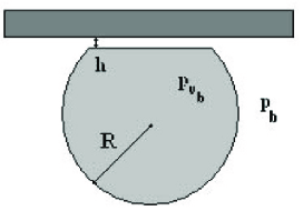
Figure 1: The bubble method of determining the disjoining pressure isotherms of wetting films (From [9], page 330).

A thin film of thickness $h$ separates a flat part of the bubble surface and the solid. The vapor bulk over the layer has a density $\rho_{v_{b}}$ and a pressure $p_{v_{b}}$. The difference between the two bulk pressures is

$$\Pi(h)=\frac{2\sigma}{R}$$

where $\sigma$ is the surface tension coefficient of the bubble; the curve $\Pi(h)$ obtained by changing the bubble radius is the so-called disjoining pressure isotherm.

Without repeating the main results of Ref. [9] related to thin liquid films, we enumerate only the properties we use to describe thin films in contact with a solid wall.
We consider the physical system at a given temperature $\theta$ and suppose that the film is thin enough such that the gravity is neglected across the interlayer.
The hydrostatic pressure in a thin liquid interlayer included between a solid wall and a vapor bulk differs from the pressure in the contiguous liquid phase.
The forces arising during the thinning of a film of uniform thickness $h$ produce the pressure $\Pi(h)$ which is equal to the difference between the pressure $p_{v_{b}}$ on the interfacial surface which is - following the expression given by Derjaguin - the pressure of the vapor mother bulk of density $\rho_{v_{b}}$, and the pressure $p_{b}$ in the liquid mother bulk of density $\rho_{b}$ from which the interlayer extends

$$\Pi(h)=p_{v_{b}}-p_{b}.$$ (1)

At equilibrium, this additional interlayer pressure $\Pi(h)$ is called the disjoining pressure.

The conditions of stability of a thin interlayer essentially depend on phases between which the film is sandwiched. In case of a single film in equilibrium with the vapor and a solid substrate, the stability condition is expressed as a form proposed in Refs. [10], [11] Chapter 4 :

$$\frac{\partial\Pi(h)}{{\partial h}}<0.$$

Let us also notice an important property of a mixture of fluid and perfect gas: the total mixture pressure is the sum of the partial pressures of components and, at equilibrium, the partial pressure of the perfect gas is constant through the liquid-vapor-gas film where the perfect gas is dissolved in the liquid phase. Calculations and results are identical to those presented in the following sections: the disjoining pressure of the mixture is the same as for the fluid without the perfect gas when a thin liquid film separates liquid and vapor phases (see Appendix).

3 Equation of motion of thin liquid films

In thin liquid films the density is strongly inhomogeneous. At temperature $\theta$ and for a given value $\mu_{0}$ of the chemical potential, the free energy of a liquid film in contact with a solid is a functional of the density $\rho$ [12]. The free energy is written in the form:

$$\digamma=\int\int\int_{D}\left(\alpha\,-\rho\mu_{0}\right)dv+\int\int_{\Sigma}\phi\,ds.$$ (2)

In this expression $D$ denotes the volume of the film and $\Sigma$ the boundary of $D$. The boundary may be a free surface (as a liquid-vapor interface bordering the film) or a solid-fluid surface. The gravity effects are neglected. Moreover,

$$\alpha\equiv\rho\,\varepsilon=K\,[\rho]$$ (3)

denotes the free volume energy of the fluid and

$$\phi=L\,[\rho]$$ (4)

denotes the surface energy. Energies $\alpha$ and $\phi$ are functionals of the fluid density $\rho$ (for example $\alpha$ and $\phi$ are both functions of the density and successive gradients of the density).
The equation of equilibrium is obtained by using the $G\hat{a}teaux$ derivative of $\digamma$:

$$\Omega-\mu_{0}=0\quad\mathrm{or}\quad\mathrm{grad}\ \Omega=0,$$ (5)

where $\Omega$ is the variational derivative of $\alpha$,

$$\Omega=\frac{\delta\alpha}{\delta\rho}.$$ (6)

We call $\Omega$ generalized chemical potential of the fluid. For examples, the following expressions of the volume free energy may be found in the literature:

• The grand potential in molecular dynamics [5]

  $$\alpha=\frac{1}{2}\int\int\int_{D_{0}}\kappa\left(\left|\mathbf{x-y}\right|\right)\,\rho\left(\mathbf{x}\right)\rho\left(\mathbf{y}\right)dv_{\mathbf{y}}.$$ (7)

  Then,

  $$\frac{\delta\alpha}{\delta\rho}=\int\int\int_{D_{0}}\kappa\left(\left|\mathbf{x-y}\right|\right)\,\rho\left(\mathbf{y}\right)dv_{\mathbf{y}}.$$

• The free energy for a generalized van der Waals theory of capillarity [3, 13, 14]

  $$\alpha=\alpha(\rho,\mathrm{{grad}\,\rho,\ldots,{grad}^{n-1}\rho,\theta).}$$ (8)

  Then,

  $$\Omega=\frac{\delta\alpha}{\delta\rho}=\frac{\partial\alpha}{\partial\rho}-\sum_{p=1}^{n-1}(-1)^{p}\mathrm{div}_{p}\left(\frac{\partial\alpha}{\partial{\mathrm{g}rad}^{p}\,\rho}\right),$$

where $\,\mathrm{{grad}^{p}}\,$ and $\,\mathrm{{div}_{p}}\,$ denotes the gradient and divergence operators iterated $p$ times.

The expression of the surface free energy functional is expressed as an expansion in Ref. [15]:

$$\phi=-\gamma_{1}\rho+\frac{\gamma_{2}}{2}\rho^{2}-\gamma_{3}\frac{d\rho}{dn}-2\gamma_{4}\,\rho\frac{d\rho}{dn}+\ldots,$$

where $\gamma_{i}\,(i=1,\ldots,4)$, are positive constants associated with intermolecular potentials between fluid and solid, the fluid density $\rho$ is calculated at the wall and $d/dn$ denotes the normal derivative to the wall.
The solution of the equilibrium problem (5) with boundary conditions coming from the variation of functional (2) determines an explicit form of the disjoining pressure. An explicit example of such a calculation based on the van der Waals square-gradient functional

$$\alpha=W(\rho)+\frac{\lambda}{2}\left|\nabla\rho\right|^{2},$$

where $W$ is the volume free energy and $\lambda$ is a constant, is given in Ref. [15].

In the general case of conservative motions, the governing equations are obtained through the Hamilton principle of stationary action [16, 17]:
Let $(t,\mathbf{x})$ be the Eulerian coordinates of particles. A particle is labeled by its position $\mathbf{X}$ in a reference space $D_{0}$. Let $D(t)$ be a corresponding material volume. The motion of a continuum is a diffeomorphism from $D_{0}$ onto $D(t)$:

$$\mathbf{x}=\varphi(t,\mathbf{X}),\quad\mathbf{X}=\chi(t,\mathbf{x}),\quad\varphi\circ\chi=\textbf{id}.$$

The equation of conservation of mass is

$$\rho\,\mathrm{det}\,F=\rho_{0}(\mathbf{X}),\quad F=\frac{\partial\varphi(t,\mathbf{X})}{\partial\mathbf{X}},$$ (9)

where $\rho_{0}$ is the density defined on $D_{0}$, and $F$ is the deformation gradient. Let us consider a one-parameter family of virtual motions

$$\mathbf{X}=\Phi(t,\mathbf{x},\eta)\quad\mathrm{with}\quad\Phi(t,\mathbf{x},0)=\chi(t,\mathbf{x})$$

where $\eta$ is a scalar defined in the vicinity of zero. The Lagrangian displacement associated with this family is [14, 16, 18]

$$\delta\mathbf{X}=\frac{\partial\Phi}{\partial\eta}(t,\mathbf{x},0).$$

The displacement vector $\delta\mathbf{X}$ is naturally defined in Eulerian coordinates. The Hamilton action is

$$a=\int_{t_{0}}^{t_{1}}\left(\int\int\int_{D(t)}\Lambda\,dv\right)dt-\int_{t_{0}}^{t_{1}}\left(\int\int_{\Sigma(t)}\phi\,dS\right)dt$$

where

$$\Lambda=\rho\left(\frac{1}{2}\,\mathbf{V}^{2}-\varepsilon\right)$$

is the Lagrangian and $\mathbf{V}$ is the velocity vector .
We consider virtual displacements $(t,\mathbf{x})\in[t_{0},t_{1}]\times D(t)\ \rightarrow\ \delta\mathbf{X}$ vanishing in a neighborhood of $\Sigma(t)$. From Eq. (9) we get :

$$\delta\rho=\rho\,\mathrm{div}_{0}\,\delta\mathbf{X}+\frac{1}{\mathrm{det}\,F}\ \frac{\partial\rho_{0}}{\partial\mathbf{X}}\ \delta\mathbf{X}$$

where $\mathrm{div}_{0}$ denotes the divergence in $D_{0}$. The definition of the Lagrange coordinates $\mathbf{X}$ implies

$$\frac{\partial\mathbf{X}(t,\mathbf{x})}{\partial\mathbf{x}}\,\mathbf{V}+\frac{\partial\mathbf{X}(t,\mathbf{x})}{\partial t}=0.$$

Then,

$$\frac{\partial\delta\mathbf{X}}{\partial\mathbf{x}}\,\mathbf{V}+\frac{\partial\mathbf{X}}{\partial\mathbf{x}}\,\delta\mathbf{V}+\frac{\partial\delta\mathbf{X}}{\partial t}=0,$$

or,

$$\delta\mathbf{V}=-F\,\frac{d\delta\mathbf{X}}{dt}$$

where

$$\frac{d}{dt}=\frac{\partial}{\partial t}+\mathbf{V}^{T}\mathrm{grad}$$

denotes the material time derivative and ^T the transposition. If we denote by $N=\displaystyle\frac{1}{2}\,\mathbf{V}^{2}-\Omega$, we obtain

$$\delta a=\int_{t_{0}}^{t_{1}}\left[\int\int\int_{D(t)}\left\{N\,\delta\rho+\rho\,\frac{d\left(\mathbf{V}^{T}F\right)}{dt}\ \delta\mathbf{X}\right\}dv\right]\,dt$$

$$=\int_{t_{0}}^{t_{1}}\left[\int\int\int_{D_{o}}\rho_{0}\left\{\frac{d\left(\mathbf{V}^{T}F\right)}{dt}-\mathrm{{grad}_{0}^{\emph{T}}\,\emph{N}}\right\}\delta\mathbf{X}\,dv_{0}\right]dt$$

where $\mathrm{{grad}_{0}}$ is the gradient in $D_{0}$.

• The Hamilton principle of least action states

  $$\forall\ (t,\mathbf{x})\in[t_{0},t_{1}]\times D(t)\ \longrightarrow\delta\mathbf{X},\mathrm{(vanishing\ in\ the\ neighborghood\ of}\ \Sigma(t)),$$

  $$\delta a\equiv\delta\int_{t_{0}}^{t_{1}}\left(\int\int\int_{D(t)}\Lambda\,dv\right)dt=0.$$

Consequently, the equation of motion is

$$\frac{d\left(\mathbf{V}^{T}F\right)}{dt}=\mathrm{{grad}_{0}^{T}\,\emph{N}.}$$

Let us note that

$$\frac{d\left(\mathbf{V}^{T}F\right)}{dt}=\left(\mathbf{\Gamma}^{T}+\mathbf{V}^{T}\frac{\partial\mathbf{V}}{\partial\mathbf{x}}\right)\,F$$

where $\mathbf{\Gamma}$ is the acceleration vector. For a conservative isothermal motion, the equation of motion is

$$\mathbf{\Gamma}+\mathrm{grad}\,\Omega=0.$$ (10)

In nonconservative cases, to take into account dissipative effects, we simply introduce a symmetric viscous stress tensor $\mathbf{\ \sigma}_{v}$ in the second member of Eq. (10); the equation of motion becomes:

$$\mathbf{\Gamma}+\mathrm{{grad\,}\Omega=\frac{1}{\rho}\,(div\,\mathbf{\ \sigma}_{v})}.$$ (11)

We consider a viscous stress tensor in the form

$$\mathbf{\ \sigma}_{v}=\kappa_{1}(\text{ tr }{D})\,\mathbf{1}+2\,\kappa_{2}\;D$$

where

$$D=\frac{1}{2}\left(\frac{\partial\mathbf{V}}{\partial\mathbf{x}}+\left(\frac{\partial\mathbf{V}}{\partial\mathbf{x}}\right)^{T}\right)$$

is the rate of deformation tensor and $\kappa_{1}$, $\kappa_{2}$ are the viscosity coefficients.
Let us notice the important property: the gradient of the generalized chemical potential $\Omega$ of thin layer is the only driving force of the liquid.

Let us remark that Refs. [1, 8] considered the liquid motion governed by the Navier-Stokes equations. The thermodynamic pressure was simply replaced with the disjoining pressure and the sign of the pressure gradient was changed in its opposite. An adherence condition was prescribed at the free liquid-vapor boundary layer.

4 Motions along a liquid nanolayer

We consider a horizontal plane liquid interlayer contiguous to its vapor bulk and in contact with a plane solid wall. We use an orthogonal system of coordinates such that the $z$-axis is perpendicular to the solid surface. The liquid film thickness is denoted by $h$.
When the liquid layer thickness $h$ is small with respect to longitudinal dimensions $L$ along the wall $\left(\epsilon=\dfrac{h}{L}\ll 1\right)$ and the inertia effects are negligeable, it is possible to simplify Eqs (11) (approximation of lubrication [19]). We denote the velocity by $\mathbf{V}=(u,v,w)^{T}$ where $(u,v)$ are the tangential components. Due to the conservation of mass, ${\partial u}/{\partial x}$, ${\partial v}/{\partial y}$ and ${\partial w}/{\partial z}$ are of the same order. The main terms associated with second derivatives of liquid velocity components correspond to ${\partial^{2}u}/{\partial z^{2}}$ and ${\partial^{2}v}/{\ \partial z^{2}}$.
In the viscous stress tensor $\mathbf{\ \sigma}_{v}=\kappa_{1}(\text{div}{\mathbf{V}})\,\mathbf{1}+2\,\kappa_{2}\;{D}$, the order of magnitude of partial derivatives implies

$$\mathbf{\ \sigma}_{v}\simeq 2\,\kappa_{2}\;{D}.$$

As in [20], we assume that the kinematic viscosity coefficient $\nu=\kappa_{2}/\rho$ depends only on the temperature. Consequently,

$$({1}/{\rho})\text{ div }\mathbf{\sigma}_{v}\simeq 2\nu\,\left\{\,\text{div }D\,+\,D\text{ grad [\thinspace Ln}\,(\rho)]\,\right\}.$$

In the liquid nanolayer, the liquid density variation $|(\rho-\rho_{b})/\rho_{b}|\ll 1$ and consequently $D$ grad{Ln ($\rho$)} is negligible with respect to div $D$. Then,

$$({1}/{\rho})\text{ div }\mathbf{\sigma}_{v}\simeq 2\,\nu\ \text{div }D.$$

Hence, in the lubrication approximation the liquid nanolayer motion verifies

$$\text{grad}\,\Omega=\nu\,\Delta{\mathbf{V}}\quad\mathrm{with}\quad\Delta{\mathbf{V}}\simeq\begin{bmatrix}\displaystyle\;\frac{\partial^{2}u}{\partial z^{2}},\displaystyle\;\frac{\partial^{2}v}{\partial z^{2}},0\end{bmatrix}.$$ (12)

We denote by $\mu(\rho)$ the phase chemical potential obtained from $\Omega$ for homogeneous densities $\rho_{l}$ and $\rho_{v}$ of a plane liquid-vapor interface without solid wall and having the same value in the liquid and vapor bulks (e.g. $\mu\left(\rho_{l}\right)=\mu(\rho_{v})=0$). In presence of a solid wall, the generalized chemical potential $\Omega$ takes a bulk value $\mu(\rho_{b})$ $=\mu(\rho_{v_{b}})=\mu_{0}$ (see Eq. (5)). The value $\rho_{v_{b}}$ is the value of the vapor density at $z\rightarrow+\infty,$ and $\rho_{b}$ is a value of the mother homogeneous fluid bulk in equilibrium with the vapor [9]. The $z$-component of Eq. (12) yields

$$\frac{\partial\Omega[\rho]}{\partial z}=0\quad{\mathrm{a}nd\ consequently}\quad\Omega[\rho]={\mu}(\rho_{b}).$$

To each value of $\rho_{b}$ (different from the liquid bulk density value $\rho_{l}$ of the plane interface at equilibrium) is associated a liquid nanolayer thickness $h$. Then, the functional $\Omega[\rho]$ is a function of $h$: $\ \Omega[\rho]=\tilde{\mu}(h)$ with $\tilde{\mu}(h)=\mu(\rho_{b}(h))$. The tangential components of Eq. (12) yield for the velocity $\mathbf{u=}(u,v)^{T}$ :

$$\mathrm{grad}\,\mu(\rho_{b})=\nu\frac{\partial^{2}\mathbf{u}}{\partial z^{2}}\ \ \ \ \Longleftrightarrow\ \ \ \frac{\partial\mu}{\partial\rho_{b}}\ \mathrm{grad}\,\rho_{b}=\ \nu\frac{\partial^{2}\mathbf{u}}{\partial z^{2}},$$ (13)

where  grad  denotes the two-dimensional gradient with respect to $(x,y)$.

Let us note that a liquid can slip on a solid wall only at a molecular level [21]. The longitudinal sizes of solid walls are several orders of magnitude higher than slipping distances and consequently, in a macroscopic mechanical model along the wall, the kinematic condition at solid walls is the adherence condition:

$$\left.{\mathbf{u}}\right|_{z=0}{=0}.$$

From the continuity of fluid tangential stresses through the liquid-vapor interface of molecular size bordering the liquid nanolayer and assuming that vapor viscosity stresses are negligible, we get

$$\;\left.\frac{\partial\mathbf{u}}{\partial z}\right|_{z=h}=0.$$

Consequently, Eq. (13) implies

$$\nu\,\mathbf{u}=\,\left(\frac{1}{2}\,z^{2}-h\,z\right)\,\mathrm{grad}\,\mu\left(\rho_{b}\right).$$

The mean spatial velocity $\overline{\mathbf{u}}$ of the liquid in the nanolayer is

$${\overline{\mathbf{u}}=\frac{1}{h}\int_{o}^{h}\mathbf{u}\ dz},$$

and consequently,

$$\nu\ {\mathbf{\overline{u}}}=-\frac{h^{2}}{3}\ \mathrm{grad}\,\mu(\rho_{b}).$$

The chemical potential is homogeneous in the bulk; then,

$$d\mu(\rho_{b})=\frac{dp\left(\rho_{b}\right)}{\rho_{b}}\,,$$

where $p\left(\rho_{b}\right)$ is the pressure corresponding to the bulk density $\rho_{b}$. Hence,

$$\mathrm{grad}\,\mu(\rho_{b})=\frac{\partial\mu}{\partial\rho_{b}}\,\frac{\partial\rho_{b}}{\partial h}\,\mathrm{grad}\,h\equiv\frac{1}{\rho_{b}}\,\frac{\partial\emph{p}(\rho_{b})}{\partial\rho_{b}}\,\frac{\partial\rho_{b}}{\partial h}\,\mathrm{grad}\,h\,.$$

The pressure $p_{v_{b}}=p\left(\rho_{v_{b}}\right)$ in the vapor bulk is constant and the disjoining pressure is

$${\Pi(h)=p\left(\rho_{v_{b}}\right)-p(\rho_{b}).}$$

Then,

$$\mathrm{grad}\,\mu(\rho_{b})=-\frac{1}{\rho_{b}}\,\mathrm{grad}\,\Pi(h)\,,$$

and we obtain

$$\chi_{b}\ {\mathbf{\overline{u}}}=\frac{h^{2}}{3}\ \text{grad}\ \Pi(h),$$ (14)

where $\chi_{b}=\rho_{b}\nu$ denotes the dynamic viscosity of the liquid. The mean liquid velocity is driven by the variation of the disjoining pressure along the solid wall and the film square thickness.

Eq. (14) is completely different from the classical hydrodynamics of films:

Indeed, for a thin liquid film, the Darcy law is ${\mathbf{\overline{u}}}=-K(h)\,{\mathrm{g}rad}\,p$,  where $p$ is the liquid pressure and $K(h)$ is the permeability coefficient. In Eq. (14), the sign is opposite and the liquid pressure is replaced with the disjoining pressure. The mass equation averaged over the liquid depth is :

$$\frac{\partial}{\partial t}\left(\int_{0}^{h}\rho\,dz\right)+\mathrm{div}\left(\int_{0}^{h}\rho\,\mathbf{u}\,dz\right)=0.$$

Since the variation of density is small, the equation for the free surface is

$$\frac{dh}{dt}+h\ \mathrm{div}{\ \mathbf{\overline{u}}}=0.$$ (15)

Replacing (14) into (15) we finally get

$$\frac{\partial h}{\partial t}+\mathrm{div}\left(\frac{h^{3}}{3\,\chi_{b}}\,\mathrm{grad}\,\Pi(h)\right)=0.$$ (16)

Eq. (16) is a non-linear parabolic equation with a good sign, if ${\ \displaystyle\frac{\partial\Pi(h)}{\partial h}<0}$. This result is in accordance with a physical stability argumentation about thin liquid layers obtained by [9, 11].

5 Conclusion

In this paper we use the variational principle of stationary action to obtain the equation of motion of a liquid in a very thin plane layer. The result is obtained whatever is the functional of free energy in the liquid and the disjoining pressure gradient is the driving force of the film motion. This result is obtained in a direct way without any phenomenological assumption as it is done in the literature where the disjoining pressure of a thin film is added formally in the equation of motion of incompressible liquids. The disjoining pressure expresses the excess free energy of the layer with respect with the superficial energy of a fluid interface (superficial tension)[22]. Consequently, in the equation of motion, the superficial tension has no raison to be taken into account. This result can be different if some curvature appears in the film as in the case of a micro droplet. We have also obtained the evolution equation for very thin isothermal flat liquid films. The thin film is driven along the substrate by the disjoining pressure gradient associated with the layer thickness. The equation of the film thickness evolution is a nonlinear parabolic equation having a good sign when the thin liquid layer is stable, the instability being probably associated with the rupture of the film along the substrate.
In appendix, we will see that the results are unchanged when the layer is constituted with a mixture of fluid and gas.

6 Appendix: Extension of results for a fluid mixture

Let us consider a mixture of the perfect gas and the non-homogeneous liquid. A mixture of the perfect gas and the saturated vapor of the liquid rises above the thin layer. To model the mixture at temperature $\theta$, we consider a volume free energy in the form [23]:

$$\rho\varepsilon=\alpha+\beta,$$

where $\alpha=K[\rho_{f}]$ is defined as in Eq. (8) and $\beta=H(\rho_{g})$ is the free volume energy of the perfect gas. The mixture density is $\rho=\rho_{f}+\rho_{g}$ where $\rho_{f}$ is the fluid density and $\rho_{g}$ is the perfect gas density.

In conservative case, without diffusion between constituents and neglecting the gravity forces, the equations of motion are [24] :

$$\left\{\begin{array}[]{c}\ \ \ \ \mathbf{\Gamma_{\emph{f}}}+\text{grad}\ \Omega[\rho_{f}]=0,\\ \ \ \ \ \mathbf{\Gamma_{\emph{g}}}+\text{grad}\ \omega(\rho_{g})=0,\end{array}\right.$$ (17)

where $\mathbf{\Gamma_{\emph{i}}}\ (i=f,g)$ are the accelerations of components, $\Omega[\rho_{f}]$ is the generalized chemical potential of the fluid (Eq. (14)) and $\omega(\rho_{g})$ is chemical potential of the perfect gas.
At equilibrium, the thin layer is invariant along the solid wall and Eq. (17₂) yields $\rho_{g}=\rho_{g0}$ where $\rho_{g0}$ is a constant in the mixture. The total pressure in the mixture bulks is the sum of the partial pressures of constituents: $p=p_{f}+p_{g}$. The partial pressure of the perfect gas is constant in the domain occupied by the mixture and the disjoining pressure is:

$$\Pi=(p_{fv}-p_{g})-(p_{fb}-p_{g})=p_{fv}-p_{fb}.$$

Hence, the disjoining pressure can be reduced to the disjoining pressure for a single inhomogeneous fluid. If we take into account the liquid viscosity and neglect the perfect gas viscosity, Eq.(17₁) becomes:

$$\mathbf{\Gamma_{\emph{f}}}+\text{grad}\ \Omega[\rho_{f}]=\nu_{f}\,\Delta\mathbf{V},$$

where $\nu_{f}$ is the fluid kinematic viscosity. This result can be extended to multi-component cases.

References

- [1] A. Oron, S.H. Davis, S.G. Bankoff, Long-scale evolution of thin liquid films, Rev. Mod. Phys. 69, 931-980 (1997).
- [2] J. Israelachvili, Intermolecular and Surface Forces, (Academic Press, New York, 1992).
- [3] B. Widom, What do we know that van der Waals did not know?, Physica A 263, 500-515 (1999).
- [4] A.A. Chernov, L.V. Mikheev, Wetting of solid surfaces by a structured simple liquid: effect of fluctuations, Phys. Rev. Lett 60, 2488-2491 (1988).
- [5] R. Evans, The nature of liquid-vapour interface and other topics in the statistical mechanics of non-uniform classical fluids, Advances in Physics 28, 143-200 (1979).
- [6] M.E. Fisher, A.J. Jin, Effective potentials, constraints, and critical wetting theory, Phys. Rev. B 44, 1430-1433 (1991).
- [7] J.S. Rowlinson, B. Widom, Molecular Theory of Capillarity, (Clarendon Press, Oxford, 1984).
- [8] B.V. Derjaguin, S.V. Nerpin, Doklady Akad. Nauk. SSSR 99, 1029 (1954) (in Russian).
- [9] B.V. Derjaguin, N.V. Churaev, V.M. Muller, Surfaces Forces, (Plenum Press, New York, 1987).
- [10] P.G. de Gennes, Wetting : statics and dynamics, Rev. Mod. Phys. 57, 827-863 (1985).
- [11] P.G. de Gennes, F. Brochard-Wyart, D. Quéré, Capillarity and Wetting Phenomena: Drops, Bubbles, Pearls, Waves, (Springer, Berlin, 2004).
- [12] H. Nakanishi, M.E. Fisher, Multicriticality of wetting, prewetting, and surface transitions, Phys. Rev. Lett. 49, 1565-1568 (1982).
- [13] M.E. Eglit, A generalization of the model of compressible fluid, J. Appl. Math. Mech. 29, 351-354 (1965)
- [14] H. Gouin, Thermodynamics form of the equation of motion for perfect fluids, Comptes Rendus Acad. Sci. Paris 305, II, 833-838 (1987).
- [15] H. Gouin, arXiv:0801.4481, Energy of interaction between solid surfaces and liquids, J. Phys. Chem. B 102, 1212-1218 (1998).
- [16] J. Serrin, Encyclopedia of Physics, Mathematical principles of classical fluid dynamics, VIII/1, (Springer, Berlin, 1959).
- [17] V.L. Berdichevsky, Variational Principles of Continuum Mechanics, Moscow, Nauka, 1983 (in Russian).
- [18] S. Gavrilyuk, H. Gouin, arXiv:0801.2333, A new form of governing equations of fluids arising from Hamilton’s principle, Int. J. Engng. Sci. 37, 1495-1520 (1999).
- [19] G. K. Batchelor, An Introduction to Fluid Dynamics, (Cambridge University Press, 1967).
- [20] Y. Rocard, Thermodynamique, (Masson, Paris, 1967).
- [21] N.V. Churaev, Thin liquid layers, Colloid. J. 58, 681-693 (1996).
- [22] Dzyaloshinsky I.E., Lifshitz E.M., Pitaevsky L.P., The general theory of van der Waals forces, Adv. Phys., 10, 165-209 (1961).
- [23] H. Gouin, arXiv:0807.4519, Variational theory of mixtures in continuum mechanics, Eur. J. Mech, B/Fluids 9, 469-491 (1990).
- [24] S. L. Gavrilyuk, H. Gouin, Yu. Perepechko, arXiv:0802.1120, Hyperbolic models of homogeneous two-fluid mixtures, Meccanica 33, 161-175 (1998).