Solitary waves of the regularized short pulse and Ostrovsky equations

Abstract

We derive a model for the propagation of short pulses in nonlinear media. The model is a higher order regularization of the short pulse equation (SPE). The regularization term arises as the next term in the expansion of the susceptibility in derivation of the SPE. Without the regularization term there do not exist traveling pulses in the class of piecewise smooth functions with one discontinuity. However, when the regularization term is added we show, for a particular parameter regime, that the equation supports smooth traveling waves which have structure similar to solitary waves of the modified KdV equation. The existence of such traveling pulses is proved via the Fenichel theory for singularly perturbed systems and a Melnikov type transversality calculation. Corresponding statements for the Ostrovsky equations are also included.

1 Introduction

The propagation of pulses in a dielectric medium is normally modeled by the nonlinear Schrödinger equation (NLSE). There are two main assumptions in the derivation of the NLSE. The first assumption is that the response of the material to electromagnetic excitation attains a quasi-steady state, the second assumption being that the pulse width is large in comparison to the scale of oscillation of the carrier frequency [21]. The experimental generation of shorter and shorter pulses means that the second assumption in the derivation of the NLSE may not be satisfied. Indeed it is possible to generate pulses whose width is just a few cycles of the carrier frequency [16]. Therefore, new models are needed for short pulse propagation. One approach to the propagation of ultra-short optical pulses is that taken by T. Schäfer and C.E. Wayne in [27]. There the authors use the full one dimensional Maxwell equations and formally derive a reduced model by assuming an experimentally determined optical susceptibility coupled with an ansatz that captures short pulses. The equation they derive is the short-pulse equation (SPE)

$$\partial_{tx}u+\alpha u+\partial_{x}^{2}u^{3}=0$$ (1.1)

where $u:(t,x)\in{\mathbb{R}}_{+}\times{\mathbb{R}}\rightarrow{\mathbb{R}}$ is the real component of the electric field in the direction transverse to the direction of propagation and $\alpha\in{\mathbb{R}}$ is a constant. It was shown there that (1.1) does not support traveling waves that are $C^{2}$ smooth. They then propose that this might reflect the Maxwell equations not possessing traveling wave solutions in the short-pulse regime or that equation (1.1) is an accurate model only for short times, and the breakdown of solutions occurs after the time of validity of (1.1) as an approximation to the Maxwell equations. We consider here another approach, namely that such traveling pulses exist if higher order terms in the approximation to the susceptibility are accounted for.

First, we strengthen the non-existence result of [27] and show there are not even piecewise smooth traveling pulses to (1.1) with a single peak. The possibility of piecewise smooth traveling waves is motivated by the development of discontinuities for the Cauchy problem for (1.1). Typically, one cannot construct global smooth solutions to hyperbolic equations such as (1.1) since discontinuities in $\partial_{t}u$ and $\partial_{x}u$ tend to develop in finite time. Since traveling waves are globally-in-time defined objects, the development of these discontinuities is a definite obstruction to the existence of smooth traveling waves. Therefore it is natural to look for traveling waves whose profiles $u(z)$ are smooth on either side of discontinuity occurring at some point $z=z_{\ast}$, and at $z_{\ast}$ an algebraic condition is satisfied so as to ensure the piecewise smooth function is a distributional solution to (1.1). In section 3 we show that the SPE does not support traveling pulses in the space of piecewise smooth functions so that scenario (iii) above is also not possible. As explained in Section 3, the main obstruction to the existence of traveling waves is the discontinuity in the right-hand side of the profile equations (4.39). Indeed, the discontinuity restricts homoclinic solutions to lie in the set $-\sqrt{c/3}<u<+\sqrt{c/3}$, whereas the jump condition requires $c=u_{\ast}^{2}$ where $c$ is the speed of the traveling wave and $u_{\ast}$ is the absolute value of $u$ immediately to the right (or equivalently left) of the discontinuity. Clearly these two conditions are not compatible. We resolve this issue by proposing a regularization mechanism which has the effect of removing the discontinuity in the profile equations as well as the need for a jump condition. The nonexistence of traveling waves (whether smooth or with discontinuities) leads us to reinvestigate the derivation of the SPE. By approximating the linear response function $\chi^{(1)}$ of the dielectric media to higher order we arrive at the regularized short pulse equation (RPSE)

$$\partial_{x}\partial_{t}u+\alpha u+\partial_{x}^{2}u^{3}+\beta\partial_{x}^{4}u=0\,.$$ (1.2)

which is the SPE (1.1) with a higher order dispersive term of strength $\beta$.

We remark here that the RSPE is similar to the Ostrovsky equation

$$\partial_{x}\left(\partial_{t}u+\partial_{x}u^{2}+\beta\partial_{x}^{3}u\right)+\alpha u=0$$ (1.3)

which was derived by L.A. Ostrovsky [23] as a model for internal solitary waves in the ocean with rotation effects of strength $\alpha<0$. The main differences being the cubic nonlinear term and both the signs and size of the physical parameters. If $\beta$ is small (1.2) is a singularly perturbed equation which induces a fast-slow structure in the equations that can be exploited by relating certain rescaled versions of the equation to other well known equations. Indeed, by setting $\tau=t/\sqrt{|\beta|}$ and $\xi=x/\sqrt{|\beta|}$, one may rewrite (1.2) as

$$\partial_{\xi}\partial_{\tau}u+\alpha|\beta|u+\partial_{\xi}^{2}u^{3}+{\rm sgn}(\beta)\partial_{\xi}^{4}u=0\,.$$ (1.4)

Setting $\beta=0$ in the RSPE with the usual scaling (1.2) yields the SPE while setting $\beta=0$ in the fast scaling (1.4) yields the modified Korteweg deVries equation (mKdV)

$$\partial_{t}u+\partial_{x}u^{3}+{\rm sgn}(\beta)\partial_{x}^{3}u=0\,.$$ (1.5)

Hence in the slow scaling the RSPE is a small perturbation of the SPE while in the fast scaling the RSPE is a small perturbation of the mKdV equation. Given this, we expect that the traveling waves $u(x-ct)$ of the RSPE, if they indeed do exist, are close to solutions of the SPE for $|x-ct|\sim{\mathcal{O}}(1/\sqrt{|\beta|})$, and close to traveling waves of mKdV for $|x-ct|\sim{\mathcal{O}}(\sqrt{|\beta|})$ with a transition region for $|x-ct|\sim{\mathcal{O}}(\sqrt{|\beta|})$. This scenario is proven via geometric singular perturbation theory in section 4.2. While in the derivation of the RSPE $\beta$ need not be small, one can nevertheless introduce a small parameter $\varepsilon$ (4.54) whereby under a suitable rescaling the equation is singularly perturbed in $\varepsilon$.

2 Derivation of the Regularized Short Pulse Equation

Consider the Maxwell equations in three space dimensions,

$$\begin{split}\partial_{t}{\bf B}=-\nabla\times{\bf E},\qquad\nabla\cdot{\bf D}=\rho\\ \partial_{t}{\bf D}=\nabla\times{\bf H}-{\bf j},\qquad\nabla\cdot{\bf B}=0\end{split}$$ (2.6)

where ${\bf E},{\bf H}:(x,t)\in{\mathbb{R}}^{3}\times{\mathbb{R}}_{+}\mapsto{\mathbb{R}}^{3}$ are the electric and magnetic fields, ${\bf D},{\bf B}:(x,t)\in{\mathbb{R}}^{3}\times{\mathbb{R}}_{+}\mapsto{\mathbb{R}}^{3}$ are the electric and magnetic flux densities, ${\bf\rho}\in{\mathbb{R}}$ is the electric charge and ${\bf j}:(x,t)\in{\mathbb{R}}^{3}\times{\mathbb{R}}_{+}\mapsto{\mathbb{R}}^{3}$ is the current density. To derive (1.2), we make several assumptions about the physical setup. The first is that the medium is a dielectric. This implies that the there are no free charges or currents. The second is that the dielectric medium is cubic and independent of space. These assumption are written as

(H1) $\hskip 14.22636pt\rho\equiv 0\;\;\;\mbox{and}\;\;\;\bf{j}=0$

(H2) $\hskip 14.22636pt{\bf B}=\mu_{0}{\bf H}\;\;\;\mbox{and}\;\;\;{\bf D}=\varepsilon_{0}{\bf E}+\varepsilon_{0}{\bf P}(x,y,z,{\bf E})$

(H3) $\hskip 14.22636pt{\bf P}(x,y,z,{\bf E})=\chi^{(1)}\ast{\bf E}+\chi^{(3)}\ast|{\bf E}|^{2}{\bf E}$

where $\mu_{0},\varepsilon_{0}$ are free space constants and $\ast$ denotes convolution in time t. Hence, Maxwell equations become

$$\begin{split}(a)&\hskip 28.45274pt\varepsilon_{0}\partial_{t}{\bf E}=\nabla\times{\bf H}-\varepsilon_{0}\partial_{t}\left\{\chi^{(1)}\ast{\bf E}+\chi^{(3)}\ast|{\bf E}|^{2}{\bf E}\right\}\\ (b)&\hskip 28.45274pt\mu_{0}\partial_{t}{\bf H}=-\nabla\times{\bf E}\end{split}$$ (2.7)

We turn (2.7) into a wave equation for ${\bf E}$, by combining the time derivative of (2.7)(a), with (2.7)(b). Recalling the identity $\nabla\times\nabla\times{\bf E}=\nabla(\nabla\cdot{\bf E})-\nabla^{2}{\bf E}$, we get

$$\nabla^{2}{\bf E}-\nabla(\nabla\cdot{\bf E})=\mu_{0}\varepsilon_{0}\partial_{t}^{2}\left({\bf E}+\chi^{(1)}\ast{\bf E}+\chi^{(3)}\ast|{\bf E}|^{2}{\bf E}\right).$$ (2.8)

We look for solutions of the form

$${\bf E}(x,y,z,t)=v(x,t){\bf E}^{\perp}(y,z,t)$$ (2.9)

where $v:{\mathbb{R}}\times{\mathbb{R}}_{+}\rightarrow{\mathbb{R}}$ and ${\bf E}^{\perp}:{\mathbb{R}}^{2}\times{\mathbb{R}}_{+}\rightarrow{\mathbb{R}}^{3}$ is given by

$${\bf E}^{\perp}=(0,E_{2},E_{3})$$

Substituting (2.9) into (2.8) yields

$$\begin{split}{\bf E}^{\perp}\left(\partial_{x}^{2}v-\mu_{0}\varepsilon_{0}\partial_{t}^{2}v\right)-\mu_{0}\varepsilon_{0}\left(2\partial_{t}v\partial_{t}{\bf E}^{\perp}+v\partial_{t}^{2}{\bf E}^{\perp}\right)+v\nabla^{2}{\bf E}^{\perp}-\nabla\left(v\nabla\cdot{\bf E}^{\perp}\right)\\ =\mu_{0}\varepsilon_{0}\partial_{t}^{2}\left(\chi^{(1)}\ast(v{\bf E}^{\perp})+\chi^{(3)}\ast(v^{3}|{\bf E}^{\perp}|^{2}{\bf E}^{\perp})\right).\end{split}$$ (2.10)

Since we are interested in the evolution of ${\bf E}$ along $x$, we can start by looking for solutions for which ${\bf E}^{\perp}(y,z,t)$ is constant vector. In this case, by simply redefining the $\chi^{(j)}$ by constants we find that the equation for the transverse evolution of the electromagnetic field satisfies the scalar one dimensional equation

$$\partial_{x}^{2}v-\mu_{0}\varepsilon_{0}\partial_{t}^{2}v=\mu_{0}\varepsilon_{0}\partial_{t}^{2}\left(\chi^{(1)}\ast v+\chi^{(3)}\ast v^{3}\right)\,.$$ (2.11)

Here we view $x$ as the evolution variable, so to put this in a form in which $t$ is the evolution variable we make the change of coordinates $(x,t)\mapsto(t,x)$ and set $(\mu_{0}\varepsilon_{0})^{-1}=:c_{0}^{2}$ to get

$$\partial_{t}^{2}v-\frac{1}{c_{0}^{2}}\partial_{x}^{2}v=\frac{1}{c_{0}^{2}}\partial_{x}^{2}\left(\chi^{(1)}\ast v+\chi^{(3)}\ast v^{3}\right)$$ (2.12)

where now $\ast$ denotes convolution with respect to $x$. It is convenient to consider the Fourier transform of (2.12) which we write as

$$\partial_{t}^{2}\hat{v}+\frac{\xi^{2}}{c_{0}^{2}}\hat{v}:=-\frac{\xi^{2}}{c_{0}^{2}}\left(\hat{\chi}^{(1)}\hat{v}+\hat{\chi}^{(3)}\widehat{v^{3}}\right)\,.$$ (2.13)

Remark 2.1

Since we are interested primarily in modeling the effect of the $\chi^{(1)}$ term, for simplicity we will assume that the $\chi^{(3)}$ response is instantaneous and modeled by the Dirac measure. Thus in (2.13) and what follows we set $\hat{\chi}^{(3)}=1$. We investigate the effect of different $\chi^{(3)}$ response functions in future work.

2.1 Approximating the $\chi^{(1)}$ Term

In dielectric materials, the $\chi^{(1)}$ term is modeled in Fourier space as [3, 21]

$$\hat{\chi}^{(1)}(\xi)=\sum_{j=1}^{n}a_{j}\left(\frac{2\xi_{j}}{\xi_{j}^{2}-\xi^{2}+\delta_{j}^{2}+2i\delta_{j}\xi}\right).$$ (2.14)

Typically for silica fibers, there are three resonances of importance which occur at practical wavelengths, namely at wavelengths of $\lambda=0.068\mu m,\lambda=0.116\mu m$ and $\lambda=9.896\mu m$. If one restricts attention to wavelengths between 0.25 and 3.5 $\mu m$, approximate values for the various constants in (2.14) can be obtained by fitting experimental data for light propagation in silica to obtain [19]

$$\hat{\chi}^{(1)}_{\rm silica}(\lambda)=\frac{0.696\lambda^{2}}{\lambda^{2}-(0.0684)^{2}}+\frac{0.4079\lambda^{2}}{\lambda^{2}-(0.116)^{2}}+\frac{0.8974\lambda^{2}}{\lambda^{2}-(9.896)^{2}}.$$ (2.15)

where $\lambda$ is the wavelength

$$\lambda=\frac{2\pi}{\xi}.$$ (2.16)

The idea in [27], developed further in this section, is that (2.15) can be expanded in powers of $\lambda$, and that the expansion is in fact a good approximation over a particular range of wavelengths. Indeed, for wavelengths between $1.6\mu m$ and $3.0\mu m$ one can approximate (2.15) by

$$\hat{\chi}_{\rm silica}^{(1)\;\tilde{\alpha},\tilde{\mu}}(\lambda)=\tilde{\mu}-\tilde{\alpha}\left(\frac{\lambda}{2\pi}\right)^{2}$$ (2.17)

for appropriate values of $\tilde{\alpha}$ and $\tilde{\mu}$ (see [27, 7] for a discussion on the validity of this approximation). Here we write an expansion of $\hat{\chi}^{(1)}$ beyond that of [27] by adding an additional term,

$$\begin{split}\hat{\chi}_{\rm silica}^{(1)\;\tilde{\alpha},\tilde{\mu},\tilde{\nu}}(\lambda)&=\hat{\chi}_{\rm silica}^{(1)\;\tilde{\alpha},\tilde{\mu}}(\lambda)-\tilde{\nu}\left(\frac{2\pi}{\lambda}\right)^{2}\\ &=\tilde{\mu}-\tilde{\alpha}\left(\frac{\lambda}{2\pi}\right)^{2}-\tilde{\nu}\left(\frac{2\pi}{\lambda}\right)^{2}\,.\end{split}$$ (2.18)

For any fixed range of wavelengths, (2.18) leads to a better approximation to (2.15) since it contains three free parameters $\tilde{\alpha},\tilde{\mu},\tilde{\nu}$ instead of just two as in (2.17). Note also that since $\lambda=2\pi/\xi$, the additional $\tilde{\nu}$ term corresponds to a higher order derivative in physical space. Finally, due to the convolution term in the nonlinear Maxwell equation (and hence the product of $\hat{\chi}^{(1)}$ and $\hat{u}$ in (2.13)), an implicit assumption in the derivation is that $\hat{u}$ is small outside the range for which $\chi^{(1)}$ is well approximated.

Recalling (2.16) and plugging the expansion for $\hat{\chi}_{\rm silica}^{(1)\;\tilde{\alpha},\tilde{\mu},\tilde{\nu}}(\xi)$ (2.18) into (2.13) and transforming back to physical variables leads to

$$\partial_{t}^{2}v-\gamma^{2}\partial_{x}^{2}v=\alpha v+\partial_{x}^{2}v^{3}+\nu\partial_{x}^{4}v$$ (2.19)

where

$$\alpha=\tilde{\alpha}/c_{0}^{2},\;\;\mu=\tilde{\mu}/c_{0}^{2},\;\;\nu=\tilde{\nu}/c_{0}^{2},\;\;\gamma^{2}=\frac{1+\tilde{\mu}}{c_{0}^{2}}\,.$$ (2.20)

2.2 Parameter Values

Up to this point we have made no mention of the signs or actual values of the parameters in (2.18). In this section we compute the signs and actual values of the parameters $\tilde{\alpha},\tilde{\mu}$, and $\tilde{\nu}$ which depend on the wavelength regime over which the $\hat{\chi}^{(1)}$ response function (2.15) is approximated. We follow the work of Schäfer and Wayne [27], in making a least-squares fit to (2.15) over the range $1.6\mu m\leq\lambda\leq 3.0\mu m$, see Fig 2.1. The sign of the parameter $\tilde{\nu}$ in (2.18) leads to a parameter regime for which our results hold. This approximation does not capture the behavior of the response function over a larger region, in particular one that includes its upwardly convex part when $\lambda<1$. A least-squares fit over the wavelength range $0.25\mu m\leq\lambda\leq 3.5\mu m$ gives a value of $\tilde{\nu}$ with the opposite sign. Our analysis does not cover this case, but we should point out that, although the approximation is better over the larger frequency range, it is not as good as the one in [27], which we use here, near the carrier frequency of interest.

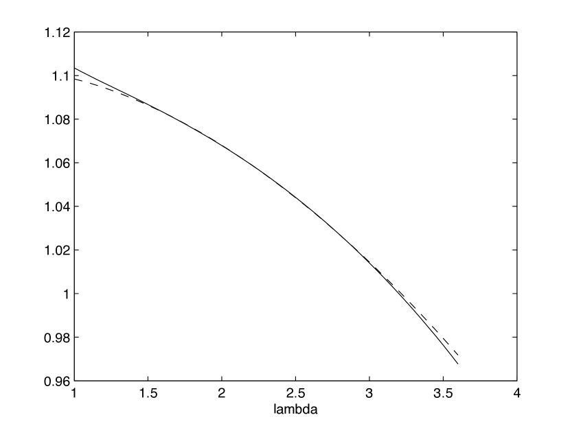
Figure 1: Approximation of the response function for silica using (2.18) with $\tilde{\alpha}=4.287786709\times 10^{-1},\;\;\tilde{\mu}=1.112628599,\;\;\tilde{\nu}=1.192774270\times 10^{-4}$. The dashed line is (2.18), the solid line is (2.15).

2.2.1 Approximation over the regime $1.6\mu m\leq\lambda\leq 3.0\mu m$

Here we compute the parameters $\tilde{\alpha},\tilde{\mu},\tilde{\nu}$ for the ansatz (2.18) by curve fitting over the exact same wavelength range as in the original paper [27]. The idea is that the extra free parameter $\tilde{\nu}$ leads to a better fit, and in addition provides a non-zero higher order regularization term. In this case the parameters obtained by a least-squares fit are

$$\tilde{\alpha}=4.287786709\times 10^{-1},\;\;\tilde{\mu}=1.112628599,\;\;\tilde{\nu}=1.192774270\times 10^{-4}\;.$$ (2.21)

In light of (2.20) this leads to an RSPE equation (1.2) with $\alpha>0,\beta>0$.

2.3 The Short Pulse Ansatz

To get (1.1) and (1.2) from (2.19) we introduce the short pulse expansion

$$v(x,t)=\delta v_{0}(x^{\delta},t^{\delta})+\delta^{2}v_{1}(x^{\delta},t^{\delta})+\cdot\cdot\cdot$$ (2.22)

where

$$x^{\delta}=\frac{x-\gamma t}{\delta}\hskip 28.45274ptt^{\delta}=\frac{\delta}{2}t.$$ (2.23)

Let

$$\nu=\beta\delta^{4},\;\;\;\delta\ll\beta$$ (2.24)

then substitution of (2.22) into (2.19) yields

$$\partial_{tx}v_{0}+\alpha v_{0}+\partial_{x}^{2}v_{0}^{3}+\beta\partial_{x}^{4}v_{0}=\mathfrak{o}(\delta)$$ (2.25)

where we have dropped the $\delta$ superscripts on $x,t$. Then to solve (2.25) to order $\delta$ we need to solve

$$\partial_{tx}v_{0}+\alpha v_{0}+\partial_{x}^{2}v_{0}^{3}+\beta\partial_{x}^{4}v_{0}=0\,.$$ (2.26)

3 General Properties of the RPSE

3.1 Conserved Quantities and Hamiltonian Formulation

While both the SPE the mKdV equation are integrable [1, 25] so associated with them are an infinite number of conserved quantities, the arguments in [10, 5] show that the $\alpha$ term in the RSPE destroys the integrable structure. Nevertheless there are conserved quantities associated with (1.2). These are the zero-mass law

$$m(u):=\int_{\mathbb{R}}u(x,t)\,dx=0,$$ (3.27)

the momentum

$$M(u):=\int_{\mathbb{R}}u^{2}\,dx$$ (3.28)

and the energy

$$H(u):=\frac{1}{2}\int_{\mathbb{R}}\alpha|\partial_{x}^{-1}u|^{2}-\frac{1}{2}|u|^{4}+\beta|\partial_{x}u|^{2}\,dx=const.$$ (3.29)

With this definition for $H$, one can regard $H$ as the Hamiltonian for the RSPE since one can write it as the gradient flow

$$\partial_{t}u={\mathcal{J}}\nabla H(u)$$ (3.30)

where ${\mathcal{J}}$ is the skew symmetric operator

$${\mathcal{J}}=-\partial_{x}\,.$$ (3.31)

3.2 Dispersive Regimes

Consider the linear RSPE equation obtained by omitting the nonlinear term,

$$\partial_{tx}u+\alpha u+\beta\partial_{x}^{4}u=0\,.$$ (3.32)

Plane waves of the form $u=Ae^{i(\xi x-\omega t)}$ are solution to (3.32) provided that the pair $(\xi,\omega)$ satisfy the dispersion relation

$$c(\xi)=\frac{\alpha}{\xi^{2}}+\beta\xi^{2}$$ (3.33)

where $c(\xi)=\omega/\xi$ is the phase speed. The dispersion relation (3.33) shows us there are two different dispersion mechanisms. For the sake of nomenclature, we call the $\alpha/\xi^{2}$ term lower-order dispersion and the $\beta\xi^{2}$ term higher-order dispersion. There are essentially four dispersive regimes one can investigate. When both lower-order and higher-order dispersion mechanisms are absent ($\alpha=\beta=0$) the RSPE reduces to a Burgers equation with nonconvex flux which is known to develop shocks (c.f. [9]). When only the lower-order dispersion mechanism is absent, the RSPE reduces to the modified KdV equation which has solitary wave solutions (corresponding to homoclinic orbits)

$$q^{0}=\sqrt{2}\mbox{sech}\left(\sqrt{\frac{c}{|\beta|}}z\right),\hskip 14.22636ptz=x-ct,\hskip 14.22636ptc,\beta>0$$ (3.34)

and traveling front solutions (corresponding to heteroclinic orbits)

$$q^{\pm}=\pm\sqrt{c}\tanh\left(\sqrt{\frac{c}{2|\beta|}}z\right),\hskip 14.22636ptz=x-ct,\hskip 14.22636ptc>0,\beta<0$$ (3.35)

When only the higher order dispersion mechanism is absent, the RSPE equation reduces to the SPE equation. Finally, we investigate the regime where both dispersion mechanisms play a role, which is the RSPE equation.

4 Solitary Waves of the SPE and RSPE

4.1 Nonexistence of Traveling Waves for the SPE

Here we prove that there do not exist piecewise smooth traveling pulse solutions to the SPE. By “pulse” here we mean that there is only one point of discontinuity. Rewrite (1.1) as the system

$$\begin{split}&(a)\hskip 28.45274pt\partial_{x}q=u\\ &(b)\hskip 28.45274pt\partial_{t}u+\alpha q+\partial_{x}u^{3}=0\end{split}$$ (4.36)

which can be thought of as an integrated version of (1.1) in the sense that one can obtain (1.1) by taking the spatial derivative of (4.36)(b). In this sense the quantity $q$ would represent the electric potential of $u$. Written this way the hyperbolic nature of the SPE is apparent in that one can view it as a correction to Burgers equation with nonconvex flux. Given this, we do not expect the existence of smooth traveling waves for (1.1) since in general the initial value problem for equations of this type tend to form discontinuities in the derivatives $\partial_{t}u$ and $\partial_{x}u$, which means we must look for distributional solutions. This has already been proven in [27]. Therefore, we look for traveling waves with profiles $(q,u)$ that are smooth on either size of a point of discontinuity $z_{\ast}$ which are distributional solutions to the original PDE (1.1). The requirement that the traveling wave be a distributional solution yields an algebraic condition that must be satisfied at the discontinuity, which are the usual Rankine-Hugoniot jump conditions. Traveling waves with these types of discontinuities are phenomena in both hyperbolic evolution equations (c.f. [8, 20]) and parabolic equations (c.f. [2, 12, 20]).

It is not hard to see that piecewise smooth functions $(q,u)$ with discontinuities across a smooth curve ${\mathcal{S}}:=\{(t,x):x=\sigma(t)\}$ with unit normal ${\bf\nu}\equiv(\nu^{1},\nu^{2})=(1+\dot{\sigma}^{2})^{-1/2}(1,-\dot{\sigma})$ are weak solutions of (4.36) if and only if (4.36) is satisfied in the classical sense on either side of ${\mathcal{S}}$ and the traces of $(q,u)$ satisfy the jump condition

$$\begin{split}&(a)\hskip 28.45274pt[[q]]=0\\ &(b)\hskip 28.45274pt\dot{\sigma}[[u]]=[[u^{3}]]\end{split}$$ (4.37)

where $[[\;\cdot\;]]$ denotes the jump across the curve ${\mathcal{S}}$.

Note that (4.37) implies $q$ is continuous across ${\mathcal{S}}$. In the case of symmetric Jumps, we can make an explicit calculation. Let $u_{\ast}\neq 0$ and suppose $u({\mathcal{S}}+0)=u_{\ast}=-u({\mathcal{S}}-0)$. Then

$$\dot{\sigma}=u_{\ast}^{2}>0.$$ (4.38)

Suppose the pair $(q,u)(z)$ is smooth on either size of $z=0$ with nonequal left- and right-hand limits at $z=0$. Then $(q,u)(z)$ is a distributional solution to (4.36) if and only if the following hold

1. $(q,u)$ satisfy the profile equations

$$\begin{split}&\dot{q}=u\\ &\dot{u}=\frac{\alpha q}{c-3u^{2}}\end{split}$$ (4.39)

pointwise in $\{z<0\}$ and $\{z>0\}$

2. The Rankine-Hugoniot conditions

$$\begin{array}[]{rcl}[[q]]&=&0\\ c[[u]]&=&[[u^{3}]]\end{array}$$ (4.40)

hold on $z=0$.

Now write the profile equations (4.39) and transmission condition (4.40) as

$$\begin{array}[]{rll}\dot{w}&=F(w)\hskip 28.45274pt\pm z>0\\ c\left[\left[w\right]\right]&=\left[\left[G(w)\right]\right]\hskip 28.45274ptz=0\end{array}$$ (4.41)

where

$$w:=\left(\begin{array}[]{c}q\\ u\end{array}\right)\hskip 28.45274ptF(w):=\left(\begin{array}[]{c}u\\ \frac{\alpha q}{c-3u^{2}}\end{array}\right)\hskip 28.45274ptG(w):=\left(\begin{array}[]{c}0\\ u^{3}\end{array}\right)$$ (4.42)

The origin $0\in{\mathbb{R}}^{2}$ is the unique fixed point of (4.41). The linearization of $F$ about the origin yields the linear system

$$\dot{w}=Aw$$ (4.43)

with

$$A=\left(\begin{array}[]{cc}0&1\\ \alpha/c&0\end{array}\right)\,.$$ (4.44)

so that it is a hyperbolic fixed point if

$$\alpha/c>0.$$ (4.45)

Since $0\in{\mathbb{R}}^{2}$ is a hyperbolic fixed point of (4.41), there exist stable and unstable manifolds ${\mathcal{W}}^{s}(0)$, ${\mathcal{W}}^{u}(0)$ which locally can be described as graphs over the stable and unstable eigenspaces $E^{s}$, $E^{u}$ of the linearized system. These manifolds can be characterized the Hamiltonian structure of the profile equations. Define $H(q,u)$ by

$$H(q,u)=\alpha q^{2}-cu^{2}+\frac{3}{2}u^{4}$$ (4.46)

Let

$$\begin{split}&(a)\hskip 28.45274pt\Sigma_{-}=\{(q,u)\in{\mathbb{R}}^{2}:|u|<\sqrt{c/3},qu\leq 0\}\\ &(b)\hskip 28.45274pt\Sigma_{+}=\{(q,u)\in{\mathbb{R}}^{2}:|u|<\sqrt{c/3},qu\geq 0\}\end{split}$$ (4.47)

and define the sets $H_{-},H_{+}$ by

$$\begin{split}&(a)\hskip 28.45274ptH_{-}:=\{H(q,u)=0\}\cap\Sigma_{-}\\ &(b)\hskip 28.45274ptH_{+}:=\{H(q,u)=0\}\cap\Sigma_{+}\\ \end{split}$$ (4.48)

It is not hard to see that $H_{-}={\mathcal{W}}^{s}(0)$ and $H_{+}={\mathcal{W}}^{u}(0)$.

Next suppose that $\overline{w}(z)$ is a piecewise smooth traveling wave. Then $\overline{w}(z)$ is defined through the stable and unstable manifolds (4.48) by

$$\overline{w}(z)=w_{-}(-z)\chi_{\{z<0\}}+w_{+}(z)\chi_{\{z>0\}}$$ (4.49)

where $w_{+}$ and $w_{-}$ are solutions to the initial value problem (4.39) with initial data

$$w_{+}^{0}=(q_{\ast},u_{\ast})\in{\mathcal{W}}^{s}(0)\hskip 56.9055ptw_{-}^{0}=(q_{\ast},-u_{\ast})\in{\mathcal{W}}^{s}(0)$$ (4.50)

and $\chi$ is the characteristic function. We will show that $\overline{w}(z)$ defined by (4.49) cannot simultaneously satisfy the jump conditions and at the same time lie within the stable and unstable manifolds for every $z\in{\mathbb{R}}$. By construction, $\overline{w}(z)$ is smooth away from $z=0$ and satisfies (4.41) on ${\mathbb{R}}/\{0\}$, thus $\overline{w}(z)$ satisfies the profile equation (4.41) pointwise on ${\mathbb{R}}/\{0\}$. Notice that by the Rankine-Hugoniot jump conditions and the fact that $(q_{\ast},u_{\ast})$ must lie on ${\mathcal{W}}^{s}(0)$, $\overline{w}$ has symmetric jumps, therefore the speed $c$ of the traveling wave $\overline{w}(z)$ is

$$c=u_{\ast}^{2}>0$$ (4.51)

However, for $u_{\ast}$ to lie in ${\mathcal{W}}^{s}(0)$ we need

$$\frac{c}{3}>u_{\ast}^{2}$$ (4.52)

which contradicts (4.51).

4.2 Existence of Solitary Waves of the RSPE and Ostrovsky Equation

Loosely speaking, the mechanism that leads to the nonexistence of traveling waves for the SPE is the discontinuous right-hand side of the profile equations. As shown in Section 4.1, the main obstruction to the existence of piecewise smooth traveling waves to the SPE is that in order for the the jump condition to hold, the value of $u$ at the jump must be larger than the allowable range $|u|<\sqrt{c/3}$ dictated by the singularity in the right-hand side of the profile equations. If one could eliminate this discontinuity, then it might be possible to obtain traveling waves. In order to eliminate the discontinuous right hand side of the profile equations, we introduced a small higher order term into the equation. This higher order term arose in expanding the susceptibility further so as to eliminate the zero wavelength singularity inherent in the derivation of the SPE. Here we study the regularized short pulse equation (1.2) and show that higher order dispersion is needed to obtain smooth pulses. For the sake of generality we will prove the theorem for general pure power nonlinearities,

$$\partial_{tx}u+\alpha u+\partial_{x}^{2}u^{k}+\beta\partial_{x}^{4}u=0.$$ (4.53)

which includes both the Ostrovsky equation (k=2) and RSPE (k=3).

We now state the main theorem of this section, the proof of which will occupy the next several subsections.

Theorem 4.1 (Existence of Traveling Waves for the RSPE)

Consider the RSPE with general pure power nonlinearity (4.53) and let

$$\varepsilon=\frac{\sqrt{|\alpha||\beta|}}{|c|}\,.$$ (4.54)

1. Suppose $k$ is an even integer and $\varepsilon$ is given by (4.54). Then for $\varepsilon>0$ small enough there exists a traveling wave solution

$$u=u(z),\;\;\;z=x-ct,\;\;\;u(z)\rightarrow 0\;\mbox{as}\;z\rightarrow\pm\infty$$ (4.55)

provided that

$${\rm sgn}(c)={\rm sgn}(\alpha)={\rm sgn}(\beta).$$ (4.56)

2. Suppose $k$ is an odd integer and $\varepsilon$ is given by (4.54). Then for $\varepsilon>0$ small enough there exists a traveling wave solution

$$u=u(z),\;\;\;z=x-ct,\;\;\;u(z)\rightarrow 0\;\mbox{as}\;z\rightarrow\pm\infty$$ (4.57)

provided that

$${\rm sgn}(c)={\rm sgn}(\alpha)={\rm sgn}(\beta)=+1.$$ (4.58)

Remark 4.1

Note that when $k$ is an odd integer, as in the RPSE, we are only able to cover the physically relevant case $\beta>0$ (see Section 2.2.1). The case $\beta<0$ is also physically relevant for RSPE (see Section 2.2, $0.25\mu m\leq\lambda\leq 3.5\mu m$) but it not considered herein.

Remark 4.2

The small parameter $\varepsilon$ is a ratio of three parameters and can be thought of as being made small by fixing two of the parameters and varying one of them. Hence by this rescaling our analysis of traveling waves of the RSPE covers the three cases (i) $\alpha$ small, (ii) $\beta$ small, and (iii) $c$ large.

Remark 4.3

Similar results can be found in [17, 18]. There the authors use variational arguments to prove the existence of a ground state traveling wave to the Ostrovsky equation for small speeds $c$. The GSPT approach used here forms the basis of work in progress [6] on the construction of multi-pulse and periodic traveling waves which are not ground states.

4.3 The Scaled Profile Equations and Fenichel Theory

Traveling wave solutions

$$u(x,t)=u(z)\hskip 28.45274ptz:=x-ct$$ (4.59)

to (4.53) must satisfy the singularly perturbed fourth order equation

$$\frac{d^{2}}{dz^{2}}\left(\beta\frac{d^{2}u}{dz^{2}}+u^{k}-cu\right)+\alpha u=0$$ (4.60)

For any $\alpha,\beta,c\neq 0$ consider the rescaling $u(z)=\tilde{u}(\tilde{z})$ where

$$\tilde{u}=|c|^{\frac{1}{1-k}}u\hskip 28.45274pt\tilde{z}=\sqrt{\frac{|c|}{|\alpha|}}z$$ (4.61)

Then upon dropping tildes the profile equations (4.60) become

$$\frac{d^{2}}{dz^{2}}\left(\varepsilon^{2}\frac{d^{2}u}{dz^{2}}+{\rm sgn}(\beta)u^{k}-{\rm sgn}(c\beta)u\right)+{\rm sgn}(\alpha\beta)u=0$$ (4.62)

where $\varepsilon$ is defined by (4.54). In order to use the GSPT framework we must rewrite the fourth order singulary perturbed equation (4.62) in standard fast-slow form. In doing this, a subtle point is the correct choice of slow and fast variables, and a correct identification and placement of the small parameter in the system of equations. The rewriting of the equation as a system is not unique, and neither is the placement of the small parameter in the equations, and hence it follows that the identification of fast and slow variables is not unique either. With this in mind, let $\varepsilon$ be as in (4.54) and set

$$u=u,\hskip 14.22636ptv=\varepsilon\dot{u},\hskip 14.22636ptw=\varepsilon v+{\rm sgn\beta}u^{k}-{\rm sgn}(\beta c)u,\hskip 14.22636pty=\dot{w}$$ (4.63)

and consider $u,v$ the fast variables and $w,y$ the slow variables. The motivation for this choice of fast and slow variables (4.63) will become clear in the subsequent analysis. We may then write the profile equations for traveling waves of (4.53) as the equivalent problem

$$\begin{array}[]{rcl}\varepsilon\dot{u}&=&v\\ \varepsilon\dot{v}&=&w+{\rm sgn}(c\beta)u-{\rm sgn}(\beta)u^{k}\\ \dot{w}&=&-y\\ \dot{y}&=&\rm{sgn}(\alpha\beta)u\end{array}$$ (4.64)

where $\cdot$ denotes differentiation with respect to the slow variable $z$. Define a fast variable $\zeta=z/\varepsilon$, then (4.64) becomes

$$\begin{array}[]{rcl}u^{\prime}&=&v\\ v^{\prime}&=&w+{\rm sgn}(c\beta)u-{\rm sgn}(\beta)u^{k}\\ w^{\prime}&=&-\varepsilon y\\ y^{\prime}&=&\varepsilon{\rm sgn}(\alpha\beta)u\end{array}$$ (4.65)

where $\prime$ denotes differentiation with respect to the fast variable $\zeta=z/\varepsilon$. We call (4.64) the slow scaling and (4.65) the fast scaling.

We prove the existence of homoclinic orbits to (4.64) (or equivalently (4.65)) via the Fenichel theory for singularly perturbed systems of ordinary differential equations, which forms the basis of geometric singular perturbation analysis. We now briefly review the Fenichel theory. For a very readable account of this theory and its applications we refer to the C.I.M.E. lectures by Jones [15] or Szmolyan [26].

Consider the system of autonomous ordinary differential equations written in standard fast-slow form

$$\begin{array}[]{rcl}\varepsilon\dot{x}&=&f(x,y;\varepsilon)\\ \dot{y}&=&g(x,y;\varepsilon)\end{array}$$ (4.66)

where $x\in{\mathbb{R}}^{n},y\in{\mathbb{R}}^{m},f,\in C^{\infty}$ and $0<\varepsilon\leq\varepsilon_{0}\ll 1$. Let $z$ denote the independent variable in (4.66), which is referred to as the slow scale. By introducing a fast scale $\zeta\equiv z/\varepsilon$ in (4.66), one obtains the equivalent system

$$\begin{array}[]{rcr}x^{\prime}&=&f(x,y;\varepsilon)\\ y^{\prime}&=&\varepsilon g(x,y;\varepsilon)\end{array}$$ (4.67)

where ${}^{\prime}\equiv\frac{d}{d\zeta}$. The basic idea of GSPT is to analyze (4.66) by combining information derived from the reduced problem

$$\begin{array}[]{rcl}0&=&f(x,y;0)\\ \dot{y}&=&g(x,y;0)\end{array}$$ (4.68)

and the layer problem

$$\begin{array}[]{rcl}x^{\prime}&=&f(x,y;0)\\ y^{\prime}&=&0\end{array}$$ (4.69)

which are the formal $\varepsilon=0$ limiting problems of (4.66) and (4.67). The fundamental connections between the formal limiting problems and (4.66) were laid down by Fenichel in [11] and consist of three main theorems referred to as Fenichel’s First, Second, and Third theorems. The basic idea of the First Theorem is that (4.68) may be seen as a dynamical system on the set ${\mathcal{M}}=\{(x,y)\in{\mathbb{R}}^{n}\times{\mathbb{R}}^{m}:f(x,y;0)=0\}$ which is an invariant manifold of fixed points for (4.69). Because of the trivial dynamics of $y^{\prime}=0$, ${\mathcal{M}}$ cannot be a hyperbolic set with respect to the full flow of (4.69). It can however be hyperbolic with respect to just the flow of $x^{\prime}=f(x,y;0)$, which leads to the concept of normal hyperbolicity.

Definition 4.1 (Normal Hyperbolicity)

A manifold ${\mathcal{M}}$ is said to normally hyperbolic with respect to a flow of the fast-slow system (4.66) if the linearization of (4.66) at any point $\rho\in{\mathcal{M}}$ when evaluated at $\varepsilon=0$ has exactly $m$ zero eigenvalues and $n$ eigenvalues $\mu$ with $\Re\mu\neq 0$.

It turns out that this assumption is enough to prove the following persistence theorem of N. Fenichel, which guarantees that ${\mathcal{M}}$ persists as a manifold ${\mathcal{M}}_{\varepsilon}$ for $\varepsilon>0$ small enough.

Theorem 4.2 (Fenichel’s First Theorem [11], [15])

Suppose ${\mathcal{M}}$ is normally hyperbolic. Then for $\varepsilon>0$ but sufficiently small, there exists a manifold ${\mathcal{M}}_{\varepsilon}$ that lies within ${\mathcal{O}}(\varepsilon)$ of ${\mathcal{M}}$ and is diffeomorphic to ${\mathcal{M}}$. Moreover, it is locally invariant under the flow of (4.66), (4.67), and $C^{k}$, including in $\varepsilon$ for any $k<+\infty$.

Attached to each point $\rho\in{\mathcal{M}}$ there is a one dimensional stable manifold ${\mathcal{W}}^{s}(\rho)$ and a one dimensional unstable manifold ${\mathcal{W}}^{s}(\rho)$. We collect these manifolds together to form stable and unstable manifolds for the full limiting slow manifold ${\mathcal{M}}$, given by

$$\begin{array}[]{rcl}{\mathcal{W}}^{s}({\mathcal{M}})&=&\bigcup_{\rho\in{\mathcal{M}}}{\mathcal{W}}^{s}(\rho)\\ {\mathcal{W}}^{u}({\mathcal{M}})&=&\bigcup_{\rho\in{\mathcal{M}}}{\mathcal{W}}^{u}(\rho)\end{array}$$ (4.70)

To address the question as to whether these structures persist when $\varepsilon>0$ we turn to Fenichel’s Second Theorem.

Theorem 4.3 (Fenichel’s Second Theorem [11, 15])

Suppose ${\mathcal{M}}$ is normally hyperbolic. Then for $\varepsilon>0$ sufficiently small, there exist a manifold ${\mathcal{W}}^{s}({\mathcal{M}}_{\varepsilon})$ (resp. ${\mathcal{W}}^{u}({\mathcal{M}}_{\varepsilon})$) that lie within ${\mathcal{O}}(\varepsilon)$ of, and is diffeomorphic to, ${\mathcal{W}}^{s}({\mathcal{M}})$ (resp. ${\mathcal{W}}^{u}({\mathcal{M}})$). Moreover, it is locally invariant under the flow of of (4.66), (4.67) and $C^{k}$, including in $\varepsilon$ for any $k<+\infty$.

Moreover, there exist stable and unstable invariant foliations with base ${\mathcal{M}}_{\varepsilon}$ with the dynamics along each foliation being a small perturbation of a suitable restriction of the dynamics of (4.69).

Theorem 4.4 (Fenichel’s Third Theorem [11, 15])

Suppose ${\mathcal{M}}$ is normally hyperbolic. Then for $\varepsilon>0$ sufficiently small there exist for each point $\rho_{\varepsilon}\in{\mathcal{M}}_{\varepsilon}$, manifolds that form an invariant family relative to (4.66), (4.67), which we name ${\mathcal{W}}^{s}(\rho)$ and ${\mathcal{W}}^{u}(\rho)$, which are within ${\mathcal{O}}(\varepsilon)$ of, and diffeomorphic to the corresponding manifolds when $\varepsilon=0$.

4.4 Construction and Analysis of the Solitary Waves

4.4.1 The Slow Manifold and Reduced Problem

When $\varepsilon=0$ in the slow scaling (4.64) we obtain

$$\begin{array}[]{rcl}0&=&v\\ 0&=&w+{\rm sgn}(c\beta)u-{\rm sgn}(\beta)u^{k}\\ \dot{w}&=&-y\\ \dot{y}&=&{\rm sgn}(\alpha\beta)u.\end{array}$$ (4.71)

Thus there is a manifold of fixed points for (4.71) which we call the critical manifold ${\mathcal{M}}_{0}$ given by

$${\mathcal{M}}_{0}=\{(u,v,w,y)\in{\mathbb{R}}^{2}\times I\times{\mathbb{R}}:u=\psi(w),v=0\}$$ (4.72)

where $\psi(w)$ is implicitly defined by the algebraic equation

$$w+{\rm sgn}(c\beta)\psi-{\rm sgn}(\beta)\psi^{k}=0$$ (4.73)

and

$$I:=\{u:{\rm sgn}(\beta)ku^{k-1})<{\rm sgn}(c\beta)\}$$ (4.74)

This means that the flow on the limiting slow manifold ${\mathcal{M}}_{0}$ is given by

$$\begin{array}[]{rcl}\dot{w}&=&-y\\ \dot{y}&=&{\rm sgn}(\alpha\beta)\psi(w).\end{array}$$ (4.75)

Proposition 4.1 (Regime of Normal Hyperbolicity of ${\mathcal{M}}_{0}$)

The critical manifold ${\mathcal{M}}_{0}$ defined through (4.72) is normally hyperbolic with respect to the flow of (4.65).

Proof. Setting $\varepsilon=0$ in the linearization of (4.65) at any point $\rho_{0}\in{\mathcal{M}}_{0}$ yields the matrix

$$\left(\begin{array}[]{ccccc}0&1&0&0\\ {\rm sgn}(c\beta)-{\rm sgn}(\beta)ku^{k-1}&0&1&0\\ 0&0&0&0\\ 0&0&0&0\\ \end{array}\right)$$ (4.76)

which has characteristic polynomial

$$\mu^{2}\left(\mu^{2}-{\rm sgn}(c\beta)+{\rm sgn}(\beta)ku^{k-1}\right)=0.$$

Hence zero is an eigenvalue of multiplicity two, and there are two distinct eigenvalues

$$\mu_{\pm}=\sqrt{{\rm sgn}(\beta)({\rm sgn}(c)-ku^{k-1})}$$

which have nonzero real part provided that

$${\rm sgn}(\beta)ku^{k-1}<{\rm sgn}(c\beta).$$ (4.77)

However, by (4.74) every point in ${\mathcal{M}}_{0}$ satisfies (4.77).
       $\Box$

Remark 4.4

Since $u$ is multivalued as a graph over $w$, the interval $I$ (4.74) is introduced to choose the branch which contains the origin.

Proposition 4.2 (Existence and Characterization of ${\mathcal{M}}_{\varepsilon}$)

Under the hypothesis of Proposition (4.1) there exists a manifold ${\mathcal{M}}_{\varepsilon}$ given by

$${\mathcal{M}}_{\varepsilon}={\mathcal{M}}_{0}+{\mathcal{O}}(\varepsilon^{2})$$ (4.78)

and the flow on ${\mathcal{M}}_{\varepsilon}$ is given by

$$\begin{array}[]{rcl}\dot{w}&=&-y\\ \dot{y}&=&{\rm sgn}(\alpha\beta)\psi(w)+{\mathcal{O}}(\varepsilon^{2})\\ \end{array}$$ (4.79)

Proof. For the regime of normal hyperbolicity of ${\mathcal{M}}_{0}$, Theorem 4.2 guarantees the existence of a manifold ${\mathcal{M}}_{\varepsilon}$ which is an ${\mathcal{O}}(\varepsilon)$ perturbation of ${\mathcal{M}}_{0}$. A straightforward calculation shows that ${\mathcal{M}}_{\varepsilon}$ is in fact an ${\mathcal{O}}(\varepsilon^{2})$ perturbation of ${\mathcal{M}}_{0}$.        $\Box$

Proposition 4.3 (Analysis of the Flow on ${\mathcal{M}}_{\varepsilon}$)

The origin of the system (4.71) is hyperbolic when viewed as a dynamical system on ${\mathcal{M}}_{\varepsilon}$ if and only if

$${\rm sgn}(\alpha)={\rm sgn}(c).$$ (4.80)

Furthermore, when (4.80) holds the origin has a one-dimensional stable and one-dimensional unstable manifold with eigenvectors of the linearization of (4.79) at the origin begin ${\mathcal{O}}(\varepsilon^{2})$ perturbations of

$$\mu_{0}=0\;\;(\text{double eigenvalue})\hskip 28.45274pt\mu_{\pm}=\pm 1$$ (4.81)

$$\eta_{0}=\left(\begin{array}[]{c}0\\ 0\\ \ast\\ \ast\end{array}\right)\hskip 28.45274pt\eta_{-}=\left(\begin{array}[]{c}\ast\\ \ast\\ -1\\ {\rm sgn}(\alpha\beta)\end{array}\right)\hskip 28.45274pt\eta_{+}=\left(\begin{array}[]{c}\ast\\ \ast\\ 1\\ {\rm sgn}(\alpha\beta)\\ \end{array}\right)$$ (4.82)

Proof. First note that the origin is an element of ${\mathcal{M}}_{0}$. Since the origin is a fixed point for the full problem (4.64) it remains a fixed point for the flow on ${\mathcal{M}}_{\varepsilon}$ also. To establish hyperbolicity of the origin as well as the eigenvectors of the linearized flow, we need only establish them for the limiting problem (4.71) or (4.75) which are $\mu=\pm\sqrt{-\psi^{\prime}(0)}$. By differentiating (4.73) we get $\psi^{\prime}(0)=-{\rm sgn}(\alpha\beta)/{\rm sgn}(c\beta)$, so that $\mu=\pm\sqrt{{\rm sgn}(\alpha){\rm sgn}(c)}$ and the result follows.
       $\Box$

4.4.2 Analysis of the Layer Problem

We now consider the fast scaling (4.65). Setting $\varepsilon=0$ we have the layer problem

$$\left.\begin{array}[]{rcl}u^{\prime}&=&v\\ v^{\prime}&=&w+{\rm sgn}(c\beta)u-{\rm sgn}(\beta)u^{k}\\ w^{\prime}&=&0\\ y^{\prime}&=&0\\ \end{array}\right\}$$ (4.83)

Essential in the construction of the traveling wave is that the layer equation has an orbit that connects points on the critical manifold ${\mathcal{M}}_{0}$. By the definition of ${\mathcal{M}}_{0}$ (4.72), this means the fixed points satisfy

$$w={\rm sgn}(\beta)u_{\ast}^{k}-{\rm sgn}(c\beta)u_{\ast}.$$ (4.84)

However, the fixed points of the layer problem must remain fixed points of the full system, and since we are looking for solutions homoclinic to the origin, we require $w=0$ which implies

$$u_{\ast}^{k-1}={\rm sgn}(c).$$ (4.85)

Note that if $k$ is odd the speed $c$ must be positive. Thus (4.83) becomes

$$\left.\begin{array}[]{rcl}u^{\prime}&=&v\\ v^{\prime}&=&{\rm sgn}(c\beta)u-{\rm sgn}(\beta)u^{k}\\ w^{\prime}&=&0\\ y^{\prime}&=&0\end{array}\right\}$$ (4.86)

If $k$ is odd the fixed points of (4.86) are $(-1,0,0,0)$, $(0,0,0,0)$, $(1,0,0,0)$ while if $k$ is even the fixed points of (4.86) are $(0,0,0,0)$ and $({\rm sgn}(c),0,0,0)$.

Proposition 4.4 (Analysis of the Layer Problem)

The layer problem (4.86) has an orbit homoclinic to the origin if and only if

$${\rm sgn}(\beta)={\rm sgn}(c)\,.$$ (4.87)

The orbit is given by

$$h(\zeta)=(q(\zeta),-q(\zeta){\rm tanh}\left(\frac{k-1}{2}\zeta\right),0,0)$$ (4.88)

where

$$q(\zeta)={\rm sgn}(c)\left(\frac{(k+1)}{2}\right)^{\frac{1}{k-1}}\,{\rm sech}^{\frac{2}{k-1}}\left(\frac{k-1}{2}\zeta\right)$$ (4.89)

and ${\rm sgn}(c)=\pm 1$ when $k$ is even while ${\rm sgn}(c)=1$ when $k$ is odd.

Proof. Since the center directions play no role in the construction of the homoclinic orbit we can restrict the flow of (4.86) to the two-dimensional $(u,v)$ phase space

$$\left.\begin{array}[]{rcl}u^{\prime}&=&v\\ v^{\prime}&=&{\rm sgn}(c\beta)u-{\rm sgn}(\beta)u^{k}\\ \end{array}\right\}$$ (4.90)

This equation is the profile of the generalized KdV (gKdV) solitary wave, which has the well known homoclinic solution (4.89) provided the sign of $c$ and $\beta$ are the same.        $\Box$

Remark 4.5

Split the parameter space into ${\mathbb{P}}={\mathbb{P}}_{-}\cup{\mathbb{P}}_{+}$ where ${\mathbb{P}}_{\pm}:=\{(\alpha,\beta,c)\in{\mathbb{R}}^{3}:{\rm sgn}(\alpha)={\rm sgn}(\beta)={\rm sgn}(c)=\pm 1,\varepsilon\ll 1\}$. From (4.85) we see that for $k$ odd, ${\rm sgn}(c)=1$ so that (4.87) implies ${\rm sgn}(\beta)=1$ and (4.80) implies ${\rm sgn}(\alpha)=1$. Thus for $k$ odd we can construct solitary waves in the parameter space ${\mathbb{P}}_{+}$ while for $k$ even we can construct solitary waves in ${\mathbb{P}}={\mathbb{P}}_{-}\cup{\mathbb{P}}_{+}$. Without loss of generality, in what follows we assume $(\alpha,\beta,c)\in{\mathbb{P}}$

4.5 Tangent Spaces and the Transversality Calculation

Now that we have analyzed the $\varepsilon=0$ limiting systems in both the slow and fast scaling, we prove the existence of solitary waves to the full $\varepsilon>0$ problem. We prove this via a reversibility argument together with a transversality calculation, which essentially entails showing that certain manifolds associated with the slow and fast orbits are transverse at $\varepsilon=0$ and thus transverse for $\varepsilon>0$ small enough.

4.5.1 The Reversibility Argument

Here we formulate and verify a condition that, together with the transversality calculation in Section 4.5.2 below, proves the existence of a homoclinic orbit of the profile equations for the RSPE equations. This condition essentially follows from reversability of the dynamical system.

Proposition 4.5 (Condition for the Existence of a Homoclinic Orbit)

Suppose $\Gamma(z):{\mathbb{R}}\rightarrow{\mathbb{R}}^{4}$ is an orbit of (4.64) (or equivalently (4.65)) which satisfies

$$\lim_{z\to-\infty}\Gamma(z)=0$$ (4.91)

and for some $z=z^{\ast}$,

$$\Pi\cap\Gamma(z^{\ast})\;\mbox{is nonempty}.$$ (4.92)

Then $\Gamma(z)$ is a homoclinic orbit.

Proof. First notice without loss of generality the translational invariance allows us to set $z^{\ast}=0$. Next, since the profile equations in both the slow scaling (4.64) and the fast scaling (4.65) are invariant under the transformation

$$z\mapsto-z\hskip 28.45274pt(u,v,w,y)\mapsto(u,-v,w,-y)$$ (4.93)

there exists a reversibility operator ${\mathcal{R}}(z)$ such that

$${\mathcal{R}}(u,v,w,y)(z)={\mathcal{R}}(u,-v,w,-y)(-z)$$ (4.94)

with $\mbox{Fix}{\mathcal{R}}$ the two dimensional plane

$$\Pi:=\{(u,v,w,y)\in{\mathbb{R}}^{4}:v=0,\;y=0\}.$$ (4.95)

One may take ${\mathcal{R}}$ as

$${\mathcal{R}}=\left(\begin{array}[]{cccc}1&0&0&0\\ 0&-1&0&0\\ 0&0&1&0\\ 0&0&0&-1\end{array}\right).$$ (4.96)

Recall that the origin of (4.64), (4.65) is a hyperbolic fixed point with two stable and two unstable eigenvalues. Clearly then there is a $\Gamma(z)$ such that $\Gamma$ satisfies (4.91). Suppose that in addition it satisfies (4.92) at the point $z=0$. This means we have constructed $\{\Gamma(z):-\infty\leq z\leq 0\}$. By applying ${\mathcal{R}}$ to this portion of $\Gamma$ we can construct $\{\Gamma(z):0\leq z\leq\infty\}$. By reversibility we have that $\Gamma(z)={\mathcal{R}}\Gamma(-z)$ so that

$$\begin{split}\lim_{z\to\infty}\Gamma(z)&=\lim_{z\to\infty}{\mathcal{R}}\Gamma(-z)\\ &={\mathcal{R}}\lim_{z\to\infty}\Gamma(-z)\\ &=0\end{split}$$ (4.97)

which by definition means $\Gamma(z)$ is a homoclinic orbit.        $\Box$

By Proposition 4.5, all that is left to prove in order to establish the existence of a homoclinic orbit to (4.64), (4.65) is that for $\varepsilon>0$ small enough there is an orbit that satisfies (4.91) and (4.92).

4.5.2 The Transversality Calculation

Consider the profile equations in the fast scaling (4.65). When $\varepsilon=0$, (4.65) has a homoclinic orbit $Q=(q,q^{\prime},0,0)$ which satisfies (4.91) and (4.92). Showing that this holds also for $\varepsilon>0$ small enough amounts to showing that the conditions for the implicit function theorem hold. This in turn amounts to showing that the evolution of the two dimensional unstable manifold under the flow of (4.65) when $\varepsilon=0$ projected onto the orthogonal complement of $\Pi$, $\Pi^{\perp}$, is nonzero.

Consider the equations in the fast scaling (4.65) in differential form notation,

$$\left.\begin{array}[]{rcl}du^{\prime}&=&dv\\ dv^{\prime}&=&dw+(1-{\rm sgn}(c)ku^{k-1})du\\ dw^{\prime}&=&-\varepsilon dy\\ dy^{\prime}&=&\varepsilon du.\\ \end{array}\right\}$$ (4.98)

where we have used Remark 4.5 to simplify the equations. Setting $\varepsilon=0$ in (4.98) yields

$$\left.\begin{array}[]{rcl}du^{\prime}&=&dv\\ dv^{\prime}&=&dw+(1-{\rm sgn}(c)ku^{k-1})du\\ dw^{\prime}&=&0\\ dy^{\prime}&=&0\\ \end{array}\right\}\,.$$ (4.99)

Consider the two form

$$dv(\zeta)\wedge dy(\zeta)\in\Lambda^{2}{\mathbb{R}}^{4}\,.$$ (4.100)

Recall that the two dimensional critical manifold ${\mathcal{M}}_{0}$ is given by

$${\mathcal{M}}_{0}:=\{(u,v,w,y)\in{\mathbb{R}}^{2}\times I\times{\mathbb{R}}:u=\psi(w),\;v=0\}.$$ (4.101)

By the Fenichel theory, the unstable (resp. stable) manifold of ${\mathcal{M}}_{\varepsilon}$ is completely foliated by smooth curves referred to as Fenichel fibers. Each Fenichel fiber intersects ${\mathcal{M}}_{0}$ at a unique point called the basepoint of the fiber. Thus, the foliation is a 2-parameter family of one-dimensional curves. The important feature of these fibers is that points on a fiber correspond to initial conditions that asymptotically approach the orbit on ${\mathcal{M}}_{0}$ as $z\rightarrow\infty$ (resp. $z\rightarrow\infty$) that passes through the basepoint of that particular fiber. Let $f^{u}(\rho_{0})$ denote an unstable fiber contained in ${\mathcal{W}}^{u}({\mathcal{M}}_{0})$ which has basepoint $\rho_{0}\in{\mathcal{M}}_{0}$ and $f^{s}(\rho_{0})$ denote a stable fiber contained in ${\mathcal{W}}^{s}({\mathcal{M}}_{0})$ which has basepoint $\rho_{0}\in{\mathcal{M}}_{0}$. The Fenichel theory enables us to identify lower-dimensional invariant manifolds within these stable and unstable manifolds. Let $\gamma_{0}\subset{\mathcal{M}}_{0}$ be an orbit on the slow manifold ${\mathcal{M}}_{0}$ satisfying $\lim_{z\rightarrow-\infty}\gamma_{0}=0$, then it has its own unstable manifold, denoted by ${\mathcal{W}}^{u}(\gamma_{0})$, which is simply the union of all unstable fibers which have their basepoints lying on $\gamma_{0}$. We now proceeds with the calculation.

Let $\eta_{1}$ be a vector tangent to the reduced problem which we take to be

$$\eta_{1}=(\psi^{\prime}(w),0,-1,{\rm sgn}(\alpha))\in T{\mathcal{W}}^{u}\,.$$ (4.102)

Since $\lim_{\zeta\rightarrow\pm\infty}w(\zeta)=0$ then by continuity

$$\lim_{\zeta\rightarrow\pm\infty}\psi^{\prime}(w)=\psi^{\prime}(0)=-1$$ (4.103)

and we can take

$$\eta_{1}=(-1,0,1,{\rm sgn}(c)).$$ (4.104)

By definition, $\eta_{1}$ is tangent to the reduced flow at $z=-\infty$. Let $\Phi^{z}=(\varphi_{1}^{z},\varphi^{z}_{2},\varphi^{z}_{3},\varphi^{z}_{4})$ denote the flow of (4.99). Then $\gamma_{0}:=\Phi^{z}\cdot\eta_{1}$ defines an orbit in ${\mathcal{M}}_{0}$. Notice that for the layer problem (4.99), for every $\zeta\in{\mathbb{R}}$ there is no flow for both $w$ and $y$ so that the third and fourth component $\eta_{1}$ is invariant under $\Phi^{z}$, that is $\Phi^{z}\cdot\eta_{1}=-\varphi^{z}_{1}\cdot(1,0,1,{\rm sgn}(\alpha))$.

Next take a vector tangent to the $\varepsilon=0$ homoclinic orbit $h$ (4.88), which we take as the vector field of the flow in the fast scaling at $\varepsilon=0$, (4.83)

$$\eta_{2}=(v,w+u-{\rm sgn}(c)u^{k},0,0).$$ (4.105)

Clearly, (4.105) gives a vector tangent to the homoclinic orbit $h$ for every $z\in{\mathbb{R}}$ and furthermore, $\eta_{2}\in T{\mathcal{W}}^{u}$. We now compute the projection of the limiting $\varepsilon=0$ fast flow onto $\Pi$ at $z=0$ when applied to the the tangent space of ${\mathcal{W}}^{u}$. That is, we wish to compute

$$(dv\wedge dy)(\eta_{1},\eta_{2})(0)\,.$$ (4.106)

To do this notice that

$$\begin{split}\frac{d}{d\zeta}\left(dv\wedge dy\right)(\eta_{1},\eta_{2})(\zeta)&=(dv^{\prime}\wedge dy)(\eta_{1},\eta_{2})(\zeta)+(dv\wedge dy^{\prime})(\eta_{1},\eta_{2})(\zeta)\\ &=(1-{\rm sgn}(c)ku^{k-1})(du\wedge dy)(\eta_{1},\eta_{2})(\zeta)+(dv\wedge 0)(\eta_{1},\eta_{2})(\zeta)\\ &=(1-{\rm sgn}(c)ku^{k-1})(du\wedge dy)(\eta_{1},\eta_{2})(\zeta)\\ &=-(1-{\rm sgn}(c)ku^{k-1})v\\ &=-(1-{\rm sgn}(c)ku^{k-1})u^{\prime}\,.\end{split}$$ (4.107)

Thus

$$\begin{split}(dv\wedge dy)(\eta_{1},\eta_{2})(0)&=\int_{-\infty}^{0}\frac{d}{d\zeta}\left(dv\wedge dy\right)(\eta_{1},\eta_{2})(\zeta)d\zeta\\ &=-\int_{-\infty}^{0}(1-{\rm sgn}(c)kq^{k-1})q^{\prime}\,d\zeta\\ &=-\left(q(0)-{\rm sgn}(c)q(0)^{k}\right)\\ &={\rm sgn}(c)\left(\frac{k-1}{k+1}\right)\left(\frac{k+1}{2}\right)^{\frac{k}{k-1}}\end{split}$$ (4.108)

which is nonzero since by assumption $\alpha,c$ nonzero. Since ${\mathcal{W}}^{u}_{\varepsilon}$ and ${\mathcal{W}}^{s}_{\varepsilon}$ intersect when $\varepsilon=0$ (4.108) shows that this intersection is transverse. Therefore, by the implicit function theorem, the manifolds still intersect for $\varepsilon>0$ small enough. The intersection of ${\mathcal{W}}^{u}_{\varepsilon}$ and ${\mathcal{W}}^{s}_{\varepsilon}$ for nonzero $\varepsilon$ finishes the construction of the pulse.
       $\Box$

4.6 The Melnikov Calculation, Homoclinic Breaking, and Asymptotic Decay of the Wave

Here we want to prove some analytic and geometric properties of the wave for $|z|$ large. In particular we want to show that the homoclinic orbit that exists when $\varepsilon>0$ enters (resp. exits) tangent to the weakly stable (resp. unstable) eigenvectors. The idea is to show that when $\varepsilon>0$ is small but nonzero, the homoclinic orbit (4.88) of the $\varepsilon=0$ layer problem breaks. That is, the one dimensional stable and unstable manifolds of the origin which intersect for the $\varepsilon=0$ layer problem, fail to intersect when $\varepsilon>0$. Thus the homoclinic orbit of the RSPE equations cannot enter (resp. exit) tangent to the eigenvectors associated with the linearization of the layer problem at the origin. This will be proved via a Melnikov calculation. Using the fact that the profile equations for RSPE are reversible, this means that the solution must enter (resp. exit) the origin tangent to the eigenvectors associated with the linearization of the reduced problem at the origin.

4.6.1 The Melnikov Integral Calculation

Here we show that the homoclinic orbit that exists in the fast scaling when $\varepsilon=0$ breaks when $\varepsilon>0$. To set up for the calculation, write the traveling wave equations in the fast scaling (4.62) as

$$\begin{array}[]{rcl}u^{\prime}&=&v\\ v^{\prime}&=&w+u-{\rm sgn}(c)u^{k}\\ w^{\prime}&=&y\\ y^{\prime}&=&-\varepsilon^{2}u\,.\end{array}$$ (4.109)

Notice here that once again the issue of the correct placement of the parameter $\varepsilon$ is important. Set $U=(u,v,w,y)$ and write (4.109) as

$$U^{\prime}=F(U;\varepsilon^{2})$$ (4.110)

with $F$ defined by the right hand side of (4.109). When $\varepsilon=0$ we have shown in Proposition 4.4 that the equations posses a homoclinic orbit $h=(q,q^{\prime},0,0)$ (4.88). By reversibility of the profile equations for the layer problem (also setting $\varepsilon=0$ in (4.109)) we see that the one dimensional stable and unstable manifolds for the layer problem intersect in the $(u,v)$ plane along $v=0$. One way to measure how much the stable and unstable manifolds of the the layer problem miss each other is to define the distance between these curves evaluated along $v=0$ which to first order is given by the Melnikov integral (4.117) which we now describe.

Consider the variational equations obtained by linearizing about the $\varepsilon=0$ homoclinic orbit $h=(q,q^{\prime},0,0)$ (4.88), given by

$$V^{\prime}=D_{U}F(h;0)V$$ (4.111)

which we write explicitly as

$$V^{\prime}=\left(\begin{array}[]{cccc}0&1&0&0\\ 1-{\rm sgn}(c)kq^{k-1}&0&1&0\\ 0&0&0&1\\ 0&0&0&0\end{array}\right)V\,.$$ (4.112)

The adjoint variational equations

$$\Psi^{\prime}=-D_{U}^{\dagger}F(h;0)\Psi$$ (4.113)

are given explicitly by the system

$$\Psi^{\prime}=\left(\begin{array}[]{cccc}0&-(1-{\rm sgn}(c)kq^{k-1})&0&0\\ -1&0&1&0\\ 0&-1&0&0\\ 0&0&-1&0\end{array}\right)\Psi\,.$$ (4.114)

where $\Psi=(\psi_{1},\psi_{2},\psi_{3},\psi_{4})$. From (4.114) we see that $\psi_{2}$ satisfies the equation

$$\psi_{2}^{\prime\prime}=1-{\rm sgn}(c)kq^{k-1}\psi_{2}$$ (4.115)

so that $\psi_{2}=q^{\prime}$ solves (4.115) since it yields the profile equations for the gKdV equation (4.90). Since $\psi_{1}=-\psi_{2}^{\prime}$, $\psi_{3}^{\prime}=-\psi_{2}$ and $\psi_{4}^{\prime}=-\psi_{3}$,

$$\Psi=\left(\begin{array}[]{c}\psi_{1}\\ \psi_{2}\\ \psi_{3}\\ \psi_{4}\end{array}\right)=\left(\begin{array}[]{c}-q^{\prime\prime}\\ q^{\prime}\\ -q\\ \int_{-\infty}^{\zeta}q\,d\zeta\end{array}\right)\,.$$ (4.116)

Let

$$M=\int_{-\infty}^{\infty}\langle D_{\varepsilon^{2}}\left.F(h(\zeta);\varepsilon^{2})\right|_{\varepsilon=0},\Psi(\zeta)\rangle$$ (4.117)

where here $\langle\;\cdot\;,\;\cdot\;\rangle$ denotes the vector inner product, and $F(h;0)$ is the vector field defined by setting $\varepsilon=0$ in the right hand side of (4.109). Note that while $D_{U}F(U;0)$ is not of full rank and thus the origin of (4.109) is not hyperbolic, $M$ defined by (4.117) nonetheless defines a Melnikov integral in the usual sense (c.f. [4]). Thus the homoclinic orbit breaks for $\varepsilon>0$ if $M\neq 0$. We now evaluate the Melnikov integral (4.117).

Clearly

$$\left.D_{\varepsilon^{2}}F(U;\varepsilon^{2})\right|_{\varepsilon=0}=\left(\begin{array}[]{c}0\\ 0\\ 0\\ q\end{array}\right)$$ (4.118)

so we have

$$\begin{split}M&=\int_{-\infty}^{\infty}\langle D_{\varepsilon^{2}}\left.F(h(\zeta);\varepsilon^{2})\right|_{\varepsilon=0},\Psi(\zeta)\rangle\\ &=-\int_{-\infty}^{\infty}q\psi_{4}\,d\zeta\\ &=-\int_{-\infty}^{\infty}q\left(\int_{-\infty}^{\zeta}q\,dz\right)\,d\zeta\\ &=-2\left(\int_{0}^{\infty}qd\zeta\right)^{2}\end{split}$$ (4.119)

Since $q\geq 0$ for all $\zeta\in{\mathbb{R}}$ we have

$$M\neq 0$$ (4.120)

which proves the result.

Remark 4.6

The geometric significance of the Melnikov calculation is that the homoclinic orbit of the full $\varepsilon>0$ problem cannot enter (resp. exit) the origin tangent to the strongly stable (resp. strongly unstable) eigenvectors. This situation is evidence of an orbit-flip bifurcation in $\varepsilon$, and allows us to construct multi-bump traveling waves [6].

Proposition 4.6 (Asymptotic Decay of the Wave.)

Assume $\varepsilon>0$ fixed and $u(z)$ is a solitary wave of (4.53). Let

$$\mu_{\varepsilon}=|\mu^{ws}_{\varepsilon}|=\mu^{wu}_{\varepsilon}=\frac{1}{2}\sqrt{2{\rm sgn}(c)-2\sqrt{1-4\varepsilon^{2}}}\,.$$ (4.121)

Then for any $m\geq 0$ there exists an $R>0$ large enough so that

$$|\partial_{z}^{m}u(z)|\leq C_{\varepsilon}e^{-\mu_{\varepsilon}|z|}$$ (4.122)

for $|z|>R$.

Proof. The Melnikov calculation coupled with the reversibility argument means that the homoclinic orbit of (4.64)(4.65) which we constructed for $\varepsilon>0$ small enough cannot enter (resp. exit) tangent to the fast directions, and so must enter (resp. exit) tangent to the slow directions. The eigenvectors associated to the slow directions have magnitude $\mu_{\varepsilon}$.        $\Box$

References

• [1] M. Ablowitz & P. Clarkson, Solitons, Nonlinear Evolution Equations and Inverse Scattering, Cambridge University Press, Cambridge, 1991.
• [2] P. W. Bates, P. C. Fife, X. Ren, & X. Wang, Traveling Waves in a Convolution Model for Phase Transitions, Archive for Rational Mechanics and Analysis, 138, Number 2 (1997).
• [3] R.W. Boyd, Nonlinear Optics, Academic Press, Boston, 1992.
• [4] S.-N. Chow, & X.-B. Lin, Bifurcation of a homoclinic orbit with a saddle-node equilibrium, Differential Integral Equations 3, (1990), no. 3, 435–466.
• [5] R. Choudhury, R.I. Ivanov, Y. Liu Hamiltonian formulation, nonintegrability, and local bifurcation for the Ostrovsky equation, Chaos, Solitons, and Fractals, 34, No. 2, (2007), 544–550.
• [6] N. Costanzino, C.K.R.T. Jones, V. Manukian, & B. Sandstede, Existence of multiple-bump traveling waves of the regularized short pulse equation, Preprint.
• [7] Y. Chung, C.K.R.T. Jones, T. Schäfer & C.E. Wayne, Ultra-short pulses in linear and nonlinear media, Nonlinearity, 18, (2005), 1351–1374.
• [8] R. Courant & K.O. Freidrichs, Supersonic flow and shock waves, Springer-Verlag, New York, 1976.
• [9] C. Dafermos, Hyberbolic Conservation Laws in Continuum Physics, Springer-Verlag, 2000.
• [10] O.A. Gilman, R. Grimshaw & Yu. A. Stepanyants, Approximate and numerical solutions of the stationary Ostrovsky equation, Stud. Appl. Math., 95, (1995), 115–126.
• [11] N. Fenichel, Geometric singular perturbation theory for ordinary differential equations, J. Diff. Eq., 31, (1979), 53–98.
• [12] P.C. Fife, Travelling waves for a nonlocal double-obstacle problem, European Journal of Applied Mathematics, 8, (1997), 581-594.
• [13] R. Grimshaw, Evolution equations for weakly nonlinear long internal waves in a rotating fluid, Stud. Appl. Math., 73, (1985), 1–33.
• [14] J.K. Hunter, Numerical solutions of some nonlinear dispersive wave equations, Lectures in Appl. Math., 26, (1990), 301–316
• [15] C.K.R.T. Jones, Geometric singular perturbation theory, in Dynamical systems: Lecture Notes in Math., 1609, Springer-Verlag, Berlin-New York, (1994), 44–118.
• [16] N. Karasawa, S. Nakamura, N. Nakagawa, M. Shibata, R. Morita, H. Shigekawa, & M. Yamashita, Comparision between theory and experiment of nonlinear propagation for a-fewcycle and ultrabroadband optical pulses in a fused-silica fiber, IEEE J. Quant. Elect., 37, (2001), 398 -404.
• [17] S. Levandovsky & Y. Liu, Stability of solitary waves of a generalized Ostrovsky equation, SIAM J. Math. Anal., 38, (2006), 985-1011.
• [18] Y. Liu & V. Varlamov, Stability of solitary waves and weak rotation limit for the Ostrovsky equation, J. Differential Equations, 203, (2004), 159 -183.
• [19] I. H. Maliton, Interspecimen comparison of the refractive index of fused silica, J. Opt. Soc. Amer., 55, October, (1965), 1205–1210.
• [20] B. P. Marchant & John Norbury, Discontinuous travelling wave solutions for certain hyperbolic systems, IMA Journal of Applied Mathematics, 67, (2002), 201-224.
• [21] A.C. Newell & J.V. Moloney, Nonlinear Optics. Addison-Wesley, Redwood City, CA, (1992).
• [22] S. P. Nikitenkova, Yu. A. Stepanyants & L. M. Chikhladze, Solutions of the modified Ostrovskii equation with cubic non-linearity, J. Appl. Maths Mechs, 64, No. 2, (2000), 267–274.
• [23] L.A. Ostrovsky, Nonlinear internal waves in a rotating ocean, Okeanologia, 18, 2 (1978), 181 -191.
• [24] J. E. Rothenberg, Space-time focusing: breakdown of the slowly varying envelope approximation in the self-focusing of femtosecond pulses, Opt. Lett., 17, (1992), 1340 -1342.
• [25] A. Sakovich & S. Sakovich, The short pulse equation is integrable, J. Phys. Soc. Jpn., 74, (2005), 239–241.
• [26] P. Szmolyan, Transversal heteroclinic and homoclinic orbits in singular perturbation problems, J. Differential Equations, 92 (1991), no. 2, 252–281.
• [27] T. Schäfer & C.E. Wayne, Propagation of ultra-short optical pulses in cubic nonlinear media, Phys. D, 196, (2004), 90 – 105.