Magnetic Properties of Young Stars in the TW Hydrae Association

Abstract

We present an analysis of infrared (IR) echelle spectra of five stars in the TW Hydrae Association (TWA). We model the Zeeman broadening in four magnetic-sensitive Ti I lines near $2.2\ \mu$m and measure the value of the photospheric magnetic field averaged over the surface of each star. To ensure that other broadening mechanisms are properly taken into account, we also inspect several magnetically insensitive CO lines near $2.3\ \mu$m and find no excess broadening above that produced by stellar rotation and instrumental broadening, providing confidence in the magnetic interpretation of the width of the Ti I lines. We then utilize our results to test the relationship between stellar magnetic flux and X-ray properties and compare the measured fields with equipartition field values. Finally, we use our results and recent results on a large sample of stars in Taurus to discuss the potential evolution of magnetic field properties between the age of Taurus ($\sim$2 Myrs) and the age of TWA ($\sim$10 Myrs). We find that the average stellar field strength increases with age; however, the total unsigned magnetic flux decreases as the stars contract onto the main-sequence.

1 Introduction

T Tauri stars (TTSs) are young, low-mass stars, which are newly formed out of their natal molecular clouds and are often associated with OB associations and/or nebulosity. The location of TTSs above the main sequence in the H-R diagram and their lithium abundance also reveal their youth. TTSs display substantial photometric and spectroscopic variability, and their properties have been reviewed by Appenzeller & Mundt (1989), Bertout (1989), Basri & Bertout (1993) and Ménard & Bertout (1999). Depending on whether they are actively accreting, TTSs are divided into two categories. Classical T Tauri stars (CTTSs) are still surrounded by dusty circumstellar disks with detectable non-stellar emission in the near-infrared (near-IR). Accretion from the disks onto the stars produces many observable features such as strong yet variable H$\alpha$ emission, often displaying P-Cygni or inverse P-Cygni profile shapes. Naked T Tauri stars (NTTSs), on the other hand, show little or no sign of accretion and do not appear to have close dusty disks around them. It is generally believed that stars evolve through a CTTS phase to become a NTTS on the way to the main sequence.

One essential piece of the puzzle to our understanding of TTSs is the stellar magnetic field. For NTTSs, it is believed that dynamo generated magnetic fields are responsible for most of their peculiarities, e.g., variable X-ray emission, flares, and cool spots. The evolution of CTTSs, especially the interaction between the stars and their circumstellar disks, is believed to be directly controlled by stellar magnetic fields (see review by Bouvier et al., 2007). Various magnetospheric accretion models (Camenzind, 1990; Königl, 1991; Collier Cameron & Campbell, 1993; Shu et al., 1994; Paatz & Camenzind, 1996) generally agree that the disks of CTTSs are truncated by stellar magnetic fields near the corotation radius and the accreting material flows along the field lines toward the polar regions of the central star. The disks of CTTSs are the birthplace for planets and the radius at which the magnetic field truncates the inner disk may determine where giant planets are halted on their inward migration in the disk (Lin et al., 1996; Eisner et al., 2005). Magnetic fields probably also play a key role in driving the stellar winds/jets seen in young stars (e.g., Shu et al., 1999). Therefore, a full understanding of the early evolution of young stars, which will lead to better understanding of both star and planet formation, requires detailed theoretical consideration and empirical measurements of the stellar magnetic field properties.

Direct detection of stellar magnetic fields is difficult, with measurements starting to become plentiful only recently (Johns-Krull, 2007). One technique, which led to the first direct detection of magnetic fields on a TTS, Tap 35 (Basri et al., 1992) and later on other stars (Guenther et al., 1999), is based on an equivalent width increase in moderately saturated magnetically sensitive lines due to Zeeman splitting. Unfortunately, this method is particularly sensitive to the choice of effective temperature and gravity used when analyzing the stellar line measurements. Another method of detecting stellar magnetic fields is through spectropolarimetry, which looks for net circular polarization in Zeeman-sensitive spectral lines. Observed along the direction that is parallel to the magnetic field, the Zeeman $\sigma$-components are circularly polarized, with the components of opposite helicity split to either side of the nominal line wavelength. If the magnetic topology on the stars is somewhat organized, there should be a measurable component along the line of sight. Reliable detections of circular polarization in TTS photospheric absoprtion lines are rare, with most recent studies finding only upper limits of $100-200$ G (Johns-Krull et al., 1999a; Daou et al., 2006; Smirnov et al., 2004). More recently, significant, but similarly weak, detections have been made (Yang et al., 2007; Donati et al., 2007) and one surprising strong detection on BP Tau has recently been published (Donati et al., 2008). On the other hand, net polarization is detected in the He I $5876$ Å emission line, first discovered by Johns-Krull et al. (1999a) on BP Tau. This He I line is believed to form in the postshock region (Hartmann et al., 1994; Edwards et al., 1994) where material accretes onto the star and the detection on BP Tau yielded a net longitudinal field of $2.46\pm 0.12$ kG in the line formation region. Circular polarization in the narrow component of the He I line has now been observed in several CTTSs (Valenti & Johns-Krull, 2004; Symington et al., 2005; Yang et al., 2007; Donati et al., 2007, 2008). These observations suggest that accretion onto CTTSs is indeed controlled by a strong stellar magnetic field.

While spectropolarimetry can provide clear detections of stellar magnetic fields, it is only sensitive to the net field resulting from the predominance of one field polarity over the other. As a result, it can miss the majority of the magnetic flux present on a star. The most successful approach so far for measuring the total magnetic flux has been to measure the Zeeman broadening of spectral lines in unpolarized light (Robinson, 1980; Saar, 1988; Valenti et al., 1995; Johns-Krull & Valenti, 1996; Johns-Krull et al., 1999b). For any given Zeeman component, the splitting resulting from the magnetic field is

$$\Delta\lambda={e\over 4\pi m_{e}c^{2}}\lambda^{2}gB=4.67\times 10^{-7}\lambda^{2}gB\,\,\,\,\,\,\rm m\mbox{\AA}\,$$

where $g$ is the Landé $g$-factor of the transition, $B$ is the strength of the magnetic field in kG, and $\lambda$ is the wavelength of the transition in Å. Johns-Krull et al. (1999b, hereafter Paper I) detected Zeeman broadening of the Ti I line at $2.2233\ \mu$m on the CTTS BP Tau and obtained a field strength of $\bar{B}=2.6\pm 0.3$ kG, averaged over the entire surface of the star. From analysis of four Ti I lines near $2.2\ \mu$m, Johns-Krull et al. (2004, hereafter Paper II) also detected a strong magnetic field of $2.5\pm 0.2$ kG on the NTTS Hubble 4. In addition, these authors examined several CO lines near $2.3\ \mu$m, which are magnetically insensitive, and found no excess broadening above that due to rotational and instrumental effects. This technique has now been used to measure the fields of 16 TTSs (Johns-Krull et al., 2004; Yang et al., 2005; Johns-Krull, 2007).

In the largest study to date of fields on TTSs, Johns-Krull (2007) used a sample of 14 stars to look for correlations between the measured magnetic field properties and stellar properties that might be important for dynamo action. No significant correlations were found and Johns-Krull (2007) speculated that the fields seen in these young stars may be entrained interstellar fields left over from the star formation process (e.g., Tayler, 1987; Moss, 2003). To supply more observational constraints and further investigate the magnetic properties of TTSs, we present here Zeeman broadening measurements of five NTTSs in the TW Hydrae association (TWA): TWA 5A, TWA 7, TWA 8A, TWA 9A and TWA 9B. At $\sim 50$ pc (Wichmann et al., 1998), TWA is the nearest region of recent star formation. Kastner et al. (1997) first concluded that a few T Tauri stars in the apparent neighborhood of TW Hya are indeed physically close to each other, based on similar X-ray emission and lithium abundance, and proposed the existence of the TW Hydrae Association. Over 20 stars have been proposed as members of TWA (though only a few of all proposed TWA members have trigonometric parallax confirmation), and a compilation of TWA members can be found in Zuckerman et al. (2004). The age for TWA is estimated at about $10$ Myrs (see discussion in Barrado Y Navascués, 2006), and it is intriguing that these pre-main-sequence stars are not associated with any molecular cloud. The origin of the TWA is still under investigation (e.g., see Makarov, 2007).

As described earlier, the magnetic field properties of TW Hya (TWA 1) have been investisgated by Yang et al. (2005, hereafter, Paper III) and Yang et al. (2007). Interstingly, Setiawan et al. (2008) report a massive planet very close to TW Hya, and Huelamo et al. (2008) argue that the observed radial velocity variations of TW Hya are best explained by a cool spot instead of a hot jupiter. Here, we study the magnetic fields of 5 additional members of TWA, utilizing infrared (IR) spectroscopy to measure Zeeman broadening in 4 Ti I lines in the K band. The observations and data reduction are presented in § 2. In § 3 we describe our data analysis technique and results, and it is followed by a discussion of the results in § 4.

2 Observations and Data Reduction

We obtained K-band IR spectra of the TWA stars at the NASA Infrared Telescope Facility (IRTF) in January 2000. Observations were made with the CSHELL spectrometer (Tokunaga et al., 1990; Greene et al., 1993) using a 0$\farcs$5 slit. With this slit width CSHELL normally delivers a spectral resolving power of $R\equiv\lambda/\Delta\lambda>40,000$. At the time our observations were taken, the resolution achieved with the 0$\farcs$5 slit was degraded due to problems within the instrument. Soon after our observing run, CSHELL was serviced to restore its spectral resolution to its nominal value. Our observations achieve an actual resolution of $R\sim 24,000$, corresponding to a FWHM of $\sim 4.5$ pixels on the $256\times 256$ InSb array detector. A continuously variable filter (CVF) isolated individual orders of the echelle grating, and a $\sim$ 0.0057 µm portion of the spectrum was recorded in each of 3 wavelength settings. The first two settings (2.2218 and 2.2291 $\mu$m) each contain 2 magnetically sensitive Ti I lines. The third setting (2.3125 $\mu$m) contains 9 strong, magnetically insensitive CO lines. Each star was observed at two positions along the slit separated by 10″. Custom IDL software described in Paper I was used to reduce the K-band spectra. The reduction includes removal of the detector bias, dark current, and night sky emission. Flat-fielding, cosmic ray removal, and optimal extraction of the stellar spectrum are also included. Wavelength calibration for each setting is based on a 3rd order polynomial fitted to $n\lambda$ for several lamp emission lines observed by changing the CVF while keeping the grating position fixed. Dividing by the order number, $n$, for each setting yields the actual wavelength scale for the setting in question. In each wavelength setting, we also observed a rapidly rotating early star to serve as a telluric standard. All spectra shown here have been corrected for telluric absorption. The IR observations are summarized in Table 1.

3 Analysis and Results

The analysis technique we employ here follows that in Papers I-III where additional details can be found. We model the profiles of four Ti I absorption lines in the K band and measure the mean magnetic field (averaged over the entire stellar surface) for the five TWA stars. Diagnostics in the IR are generally more sensitive to Zeeman broadening than lines in the optical thanks to the $\lambda^{2}$ dependence of magnetic splitting (see eq.[1]) compared with the $\lambda^{1}$ dependence of Doppler broadening mechanisms. Using estimates of the key stellar parameters of our objects, namely, $T_{\rm eff}$, $\log g$, [M/H] and $v\sin i$, we first construct model atmospheres and synthesize the Ti I line profiles without the presence of magnetic fields. The observed magnetically insensitive CO lines are also synthesized to show that instrumental and rotational broadening are properly taken into account and the non-magnetic spectrum is accurately predicted. There are no free parameters involved in computing the non-magnetic line profiles. The excess broadening seen in the Ti I lines relative to the non-magnetic model is interpreted as Zeeman broadening. Fitting the magnetically broadened Ti I line profiles then yields the average magnetic field strength on the stellar surface.

Paper III presented extensive tests of this analysis technique to quantify possible systematic errors resulting from inaccurate stellar parameters. The Monte Carlo analysis showed that a 200 K error in $T_{\rm eff}$ or 0.5 dex error in $\log g$ introduces only about $10\%$ or less systematic error in the derived mean field measurements. This is because we are modeling actual Zeeman broadening instead of some other effect such as a change in equivalent width which is particularly sensitive to errors in $T_{\rm eff}$ and $\log g$. Thus, instead of performing a detailed spectral analysis to determine the stellar parameters as in our previous studies (e.g., Papers I-III), we adopt the most accurate values available in the literature for our targets. Values for these non-magnetic stellar parameters are given in Table 2 and justified in subsequent subsections for each star.

The CO lines near $2.3\ \mu$m serve as an excellent verification of our chosen stellar parameters. For each of our targets, we interpolate a grid of the “next generation” (NextGen) atmospheres of Allard & Hauschildt (1995) to the specific values of $T_{\rm eff}$, $\log g$ and [M/H] and construct a model atmosphere appropriate for the star. We then synthesize the CO line profiles and convolve them with a Gaussian corresponding to the resolution of the observed spectrum. The CO line data are taken from Goorvitch (1994) for the CO X $\Sigma^{+}$ lines. No stellar parameter fitting is involved with the synthesis of the CO lines. Continuum normalization is the only free parameter used to match the observed and synthetic spectra. The shape, especially the widths, of the synthetic line profiles is solely determined by the stellar parameters. A good match between the widths of the synthetic CO lines and that of the observations, as seen in the bottom panels of Figures 1 and $3-6$, shows that the dominant non-magnetic broadening mechanisms are properly taken into account.

A polarized radiative transfer code (Piskunov, 1999) is utilized to compute the line profiles for both the CO and Ti I lines, assuming a radial magnetic field geometry in the photosphere. To construct our models, we treat the stellar surface as if it is divided into a number of regions, where one region is field-free and the other regions are each covered by a single magnetic field strength. The fractional size of each region is specified by a filling factor and the total of the filling factors must be unity. These regions are assumed to be spatially well mixed over the surface of the star. We compute the spectrum for each region, and the spectra of all regions are multiplied by their corresponding filling factors and summed up to form the final model spectrum for a specific set of field strengths and filling factors. We use the nonlinear least-squares technique of Marquardt (Bevington & Robinson, 1992) to solve for the best-fit combination of field strengths and filling factors as described below.

For each target, we fit three different models. The first model (hereafter, M1) allows a single magnetic field strength ($B$) to cover a fraction of the stellar surface ($f$), and the rest of the surface is field-free. The mean stellar magnetic field, $\bar{B}$, is just $Bf$. The free parameters of this model are $B$ and $f$. The second model (hereafter, M2) divides the surface of the star into three regions: two regions covered with magnetic fields of different strengths ($B_{1}$, $B_{2}$) and filling factors ($f_{1}$, $f_{2}$), and one region with no magnetic field. The mean magnetic field on the stellar surface for M2 is $\bar{B}=B_{1}f_{1}+B_{2}f_{2}$. The free parameters of this model are $B_{1}$, $f_{1}$, $B_{2}$ and $f_{2}$. The third model (hereafter, M3) allows three magnetic regions on the stellar surface to have specific field strengths of 2 kG, 4 kG and 6 kG, respectively. The rest of the surface is field-free. Only the filling factors are solved for in this model. The mean field is then $\bar{B}=\displaystyle\sum_{i=1}^{3}B_{i}f_{i}$.

As discussed in Paper I-III, the M1 model provides a much better fit to the observations than models with no magnetic broadening, but the model M1 profile is not as smooth and broad as the observed line profile, and is incapable of supplying good fits for the cores and the wings of the lines simultaneously. The magnetic structure on the surface of TTSs is unlikely to be so simple, and this is the motivation to add more magnetic components in model M2 and M3, which provides improved smoother fits to the observed line profiles. Due to lower spectral resolution ($\sim 24,000$) than that in Paper I-III ($\sim 36,000$), the need for more magnetic components is less urgent. For example, likely due to the lower spectral resolution achieved here, the data do not clearly require a model with 3 magnetic components as in M3; however, we fit such a model to be consistent with previous work in order to avoid any systematic differences when comparing the field measurements of TWA stars with previous results. Below, we discuss the results for each of our targets in detail.

3.1 TWA 5A

TWA 5 is among the five original TWA members reported by Kastner et al. (1997). Webb et al. (1999) discovered a M8.5 brown dwarf companion, TWA 5B, $\sim 2^{\prime\prime}$ away from the much brighter TWA 5A (M1.5). Macintosh et al. (2001), using adaptive optics (AO) imaging, found that TWA 5A itself is also a close binary system with a separation of $\sim 0\farcs 06$ at that time. Konopacky et al. (2007) monitored the TWA 5Aab system for five years. Their speckle and AO observations yield an orbital solution with a semi-major axis of $0\farcs 066\pm 0\farcs 005$ and a period of $5.94\pm 0.09$ yrs. These authors also find a K band flux ratio of $\sim 1.25$, so we are most likely seeing substantial light from both stars in our spectra.

It is also suspected that there is possibly another spectroscopic component in the TWA 5Aab pair, causing large radial velocity variations (Torres et al., 2003). We do notice peculiarities in our spectra of TWA 5Aab system, which is shown in Figure 1. The three wavelength settings shown here were observed on 3 consecutive nights. The two Ti I line profiles in the $2.2300\ \mu$m setting are very asymmetric, and some of the CO lines show large wavelength shifts or asymmetries as well. With a period of about 6 years, the line profiles of the binary system obtained on consecutive nights should not vary so dramatically. This drastic change may be caused by a third component in the TWA 5Aab system in a close orbit with one of the two known members.

We do not notice obvious asymmetry in the two Ti I line profiles in the $2.2228\ \mu$m setting, so these two lines are used for magnetic field measurement. Following Weintraub et al. (2000), we adopt an effective temperature of 3700 K and derive a $\log g$ of 3.7 from their absolute magnitude and stellar mass estimates, which assume a distance of $55\pm 9$ pc (Webb et al., 1999). A $v\sin i$ of 38 km s^-1 is adopted from Torres et al. (2003). The measured mean magnetic field values of TWA 5A along with that of the other four TWA stars, using the three different models, are listed in Table 2. The reduced $\chi^{2}$ values for TWA 5A given in Table 2 are calculated with all four Ti I lines included so that it is consistent with other stars. Note that only the two lines in the $2.2228\ \mu$m region are fitted and the reduced $\chi^{2}$ values calculated with these two lines only are 1.06, 1.10 and 1.28 for models M1-M3, repectively. The observed and the best fit model spectra of TWA 5A are shown in Figure 1. Given the uncertainties associated with the number of stars in this system, we report our field estimate here (which is likely some sort of average of all the stars present) but do not use measurements of this system in any subsequent analysis.

3.2 TWA 7

TWA 7 was discovered as a TWA member by Webb et al. (1999). Neuhäuser et al. (2000) detected a possible extra-solar planet candidate about 2$\farcs$5 away from TWA 7 using ground-based direct imaging, but they concluded that this object is more likely an unrelated background source. This interpretation was later confirmed by the coronagraphic observations of Lowrance et al. (2005). An inclination of $28^{\circ}$ is estimated for TWA 7.

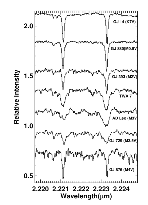
Figure 2: Spectra of TWA 7 along with several spectral type standards in the $2.2228\ \mu$m setting. The spectra are all vertically offset for better display. Note that both AD Leo and GJ 729 are known to have strong magnetic fields (Johns-Krull & Valenti, 2000). See also earlier measurements for AD Leo by Saar & Linsky (1985), and GJ 729 by Johns-Krull & Valenti (1996).

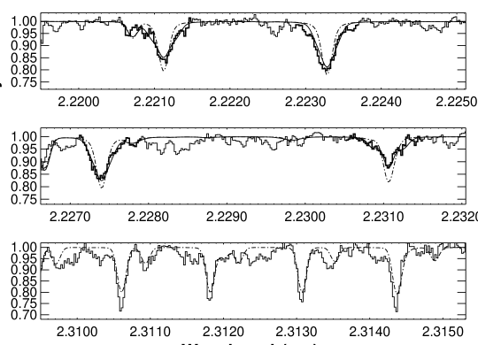
Figure 3: Best fit of infrared spectra of TWA 7 using the two-magnetic-component model M2. Top two panels: magnetically sensitive Ti I lines; Bottom panel: magnetically insensitive CO lines. (Histogram: data; dash-dotted line: fit without magnetic field; smooth line: fit with magnetic broadening.)

Webb et al. (1999) determined a spectral type of M1 for TWA 7 by comparing their low resolution optical spectra with spectral standards from Montes & Martin (1998). In our high resolution IR data, we notice that some molecular lines of TWA $7$ in the K band are more prominent than that indicated by a M1 spectral type. Shown in Figure 2, we compare the spectrum of TWA $7$ in the $2.2228\ \mu$m setting with that of several stars of different spectral types. From this TWA 7 appears to be of later spectral type than M1, probably closer to M3. Though we do not synthsize molecular lines in this wavelength setting, the Ti I lines are not seriously blended with these features. The molecular lines, possibly CN, do not substantially affect our magnetic field measurement. In our analysis we adopt a $T_{\rm eff}$ of 3300 K for TWA 7, appropriate for an M3 star, and a $\log g$ $=3.85$ is derived by adopting the bolometric luminosity and stellar mass estimates of Neuhäuser et al. (2000). The conversion of spectral type to effective temperature in this paper is based on Johnson (1966). Interestingly, Johnson’s spectral type to $T_{\rm eff}$ conversions closely parallel those derived for young stars by Luhman et al. (2003), from G through mid-M spectral types. We use a $v\sin i$ $=9.0$ km s^-1, which is slightly larger than previous measured value of $6.1\pm 0.5$ km s^-1 from Neuhäuser et al. (2000). Our choices of $v\sin i$ are based initially on literature values and in some cases they are adjusted by a small amount to better match the width of the observed nonmagnetic CO lines. As mentioned above, our analysis technique suffers $\sim 10\%$ or less systematic error for a 200 K error in $T_{\rm eff}$ or 0.5 dex error in $\log g$, so the measured field values of TWA 7 are not subject to much change, whether its spectral type is M1 or M3. The best fit for TWA 7 is shown in Figure 3.

3.3 TWA 8A

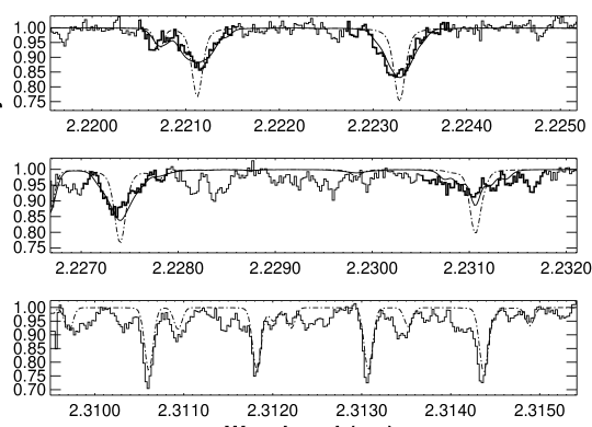
Figure 4: Best fit of infrared spectra of TWA 8A using the two-magnetic-component model M2. Top two panels: magnetically sensitive Ti I lines; Bottom panel: magnetically insensitive CO lines. (Histogram: data; dash-dotted line: fit without magnetic field; smooth line: fit with magnetic broadening.)

TWA 8A was also identified by Webb et al. (1999) as an association member, and is classified as a M2 star. Its fainter companion TWA 8B is about $13\arcsec$ to the south of the primary. The membership of the companion in TWA is based primarily on its similar lithium abundance and radial velocity compared to other members of the association. Trigonometric parallax and proper motion measurements are needed for further confirmation. White & Hillenbrand (2004) derive a spectral type of M3 ($\pm 0.5$) for TWA 8A, by matching line and molecular band ratios to those of dwarf spectral standards which are rotationally broadened. These authors also determined an upper limit of 5.5 km s^-1 for the $v\sin i$ of TWA 8A. For our analysis, we use a $T_{\rm eff}$ of 3400 K, $\log g$ of 4.0, and $v\sin i$ of 4.0 km s^-1. The inclination of TWA 8A is estimated to be $16^{\circ}$, so it is seen close to pole-on. The best fit for the Ti I lines as well as the predicted CO spectrum of TWA 8A are shown compared with the observed spectra in Figure 4.

3.4 TWA 9A & 9B

TWA 9 (CD $-36^{\circ}7429$) was found by Jensen et al. (1998) to be in the physical vicinity of TW Hya. It is a binary system with a separation of $6\arcsec$. The Hipparcos satellite (ESA, 1997) measured a distance of $50.3\pm 6.0$ pc for TWA 9 system. In the literature, TWA 9A is classified either as K5 (Webb et al., 1999) or K7 ($\pm\ 1$) (White & Hillenbrand, 2004). Previously reported $v\sin i$ values are $7\pm 3\ \mbox{km s${}^{-1}$}$ (Reid, 2003) and $11\pm 1\ \mbox{km s${}^{-1}$}\$ (White & Hillenbrand, 2004) for TWA 9A. We adopt $T_{\rm eff}$ = 4000 K and $\log g$ = 4.5, and use $v\sin i$ = 9 km s^-1. The inclination angle of TWA 9A is inferred to be $90^{\circ}$.

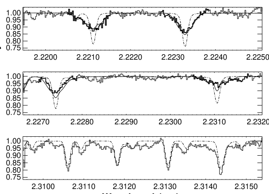
Figure 5: Best fit of infrared spectra of TWA 9A using the two-magnetic-component model M2. Top two panels: magnetically sensitive Ti I lines; Bottom panel: magnetically insensitive CO lines. (Histogram: data; dash-dotted line: fit without magnetic field; smooth line: fit with magnetic broadening.)

For TWA 9B, reported spectral types include M1 (Webb et al., 1999) and M3.5 ($\pm\ 0.5$) (White & Hillenbrand, 2004), and $v\sin i$ values of $4\pm 3\ \mbox{km s${}^{-1}$}$ (Reid, 2003) as well as $9\pm 1\ \mbox{km s${}^{-1}$}$ (White & Hillenbrand, 2004) have been published. We use $T_{\rm eff}$ = 3400 K, $\log g$ = 4.0, and $v\sin i$ = 10 km s^-1. The inclination angle is estimated to be $60^{\circ}$. Due to the very poor signal-to-noise ratio we obtain on this star, the spectrum in the $2.2300\ \mu$m setting is excluded from our analysis. The best fit spectra along with observed spectra of TWA 9A and TWA 9B are shown in Figure 5 and 6, respectively.

4 Discussion

By fitting the Zeeman broadening in the magnetically sensitive Ti I lines, we measure the average surface magnetic field of five TWA stars. Three different models were used to fit the line profiles and measure the magnetic field strength with generally good agreement in the results between the three. Model M1 assumes only 1 magnetic component to the stellar atmosphere. This model provides a good match to TWA 5A in the $2.2228\mu$m region (but not the $2.2300\mu$m region). This is likely due to the fact that TWA 5A apparently has a relatively large $v$sin$i$ so that rotational broadening, in addition to the magnetic broadening, strongly affects the line profile shapes. Because our magnetic models for TWA 5A do not reproduce line profiles in the $2.2300\mu$m region, our derived magnetic properties for TWA 5A may have large systematic errors. Generally, mean field strength increases as more components are added to the model, which suggests that the observed profiles have wings that are too broad to be fit by a single component. For the other stars, the lowest reduced $\chi^{2}$ typically occurs for model M2, though M3 is favored in one case. However, there is generally quite good agreement bewteen the mean field values recovered using these two models with the difference bewteen them averaging 15%. For consistency with previous studies, we use the results from M3 when comparing to results found by Johns-Krull (2007).

Theoretically, equipartition arguments for the Sun and cool stars suggest that the magnetic field strength should scale with the gas pressure in the surrounding non-magnetic photosphere which sets a limit for the maximum field strength allowed on the star (e.g. Spruit & Zweibel, 1979; Safier, 1999). Rajaguru et al. (2002) found that in the regime where convectively stable flux tubes exist, equipartition pressure allows a maximum magnetic field strength of $\sim 1300$ G for values of $T_{\rm eff}$ and $\log g$ appropriate for most of our TWA stars. We calculate equipartition field strengths for the TWA stars by balancing magnetic pressure, $B_{eq}^{2}/(8\pi)$, with the gas pressure in surrounding unmagnetized photosphere, $P_{g}$. We use the gas pressure at the level in the atmosphere where the local temperature is equal to the effective temperature in the model atmospheres used for our stars. This should be an upper limit for gas pressure because this level is approximately where the continuum forms, while the Ti I lines form over a wide range of depths above this level in the atmosphere. The equipartition field strengths, $B_{eq}={(8\pi P_{g})}^{1/2}$, of the TWA stars are listed in the last column of Table 2. These values are in good agreement with the estimate from Rajaguru et al. (2002). Compared with the measured mean field values, they are all smaller by a factor of at least 1.38 and more typically $\sim 2.0$ (for model M2), suggesting that magnetic pressure dominates over gas pressure in the photospheres of the TWA stars observed here. This in turn implies complete coverage of magnetic fields over surface of these stars. Magnetic regions with excess pressure would expand, while field free regions contract into the lower pressure nonmagnetic regions until equipartition is established at a lower field strength or until the entire star is covered with magnetic fields. As discussed in Papers I and II, our models do not necessarily require field-free regions. The results are essentially the same with or without a 0 kG field component. As an example, we fit the observed spectra of TWA 8A with a model which allows on the stellar surface no field-free region and four magnetic regions with specific field strengths of 1 kG, 3 kG, 5 kG and 7 kG. The measured magnetic field value using this model is 3.4 kG with a reduced $\chi^{2}$ of 1.22, while model M3 yields 3.3 kG with a reduced $\chi^{2}$ of 1.25 (see Table 2). With a field-free region included in our current analysis, all the TWA stars have at least $76\%$, in most cases $80\%-86\%$, of their surfaces covered with magnetic fields. The surfaces of TTSs are quite possibly fully covered by strong magnetic fields.

Pevtsov et al. (2003) examine the X-ray luminosities and the total unsigned magnetic flux of active stars as well as regions of different activity level on the Sun. They find a nearly linear correlation over many decades of variation in the two quantities. We calculate the magnetic flux of the four TWA stars (excluding TWA 5A since it is an unresolved multiple system), using our magnetic field measurements and the stellar radii estimated from bolometric luminosities given in Webb et al. (1999) and the effective temperatures of our stars. We utilize the X-ray luminosity-magnetic flux relationship of Pevtsov et al. (2003) and calculate the predicted X-ray luminosity. For comparison, we use the X-ray to bolometric luminosity ratio, $L_{x}/L_{bol}$, reported by Webb et al. (1999) to get the value of $L_{x}$ for each star. The predicted and measured values of $L_{x}$ for the three TWA stars (TWA 7, TWA 8A and TWA 9A) presented in this paper and that of TW Hydrae taken from Paper III are plotted in Figure 7. A measured value for TWA 9B is not available in the literature. As shown in Figure. 7, the observed $L_{x}$ values of the four TWA stars are smaller than the predicted values by a factor of $2.7\pm 0.7$ on average. This is similar to the findings of Johns-Krull (2007) in a study of 14 CTTSs in Taurus and Auriga. The stars from Johns-Krull (2007) are also plotted in Figure 7, and the difference between the observed and the predicted $L_{x}$ values is a bit more obvious. The average ratio of the predicted to observed $L_{x}$ values is $17.7\pm 3.4$ for the 14 Taurus and Auriga stars. At an age of about 10 Myrs, the TWA stars are substantially older than the stars in the Taurus-Auriga region ( $\sim$2 Myrs). As a result, the TWA stars are substantially closer to the main sequence and this may be the reason why their X-ray luminosities and magnetic flux values are closer to the relationship found by Pevtsov et al. (2003) which was based primarily on main sequence stars. The X-ray emission on active stars such as TTSs is thought to mainly result from energy dissipation in magnetic fields during flares and small-scale flare-like activities (Güdel et al., 2003; Arzner et al., 2007). Magnetic fields are stressed due to convective gas motions in the lower photosphere and below (Foukal, 2004), producing flares of various scales. For PMS stars that are fully covered by magnetic fields, when the magnetic field strength is larger than the equipartition value, it may be more difficult for the gas, at least in the photosphere, to push around the fields and build up magnetic stress. This would be the case for both the Taurus stars and the TWA stars. The ratio of the observed to equipartion magnetic field, $B_{obs}/B_{eq}$, for the Taurus stars on average is greater than that for the TWA stars, so the X-ray production might be more prohibited for the Taurus stars resulting in the observed $L_{x}$ being further away from the line of equality in Figure 7. It will be interesting to see where TTSs in other age groups fit in this picture relating magnetic flux and X-ray emission.

The origin of magnetic fields on TTSs has sparked various theoretical speculations, but it is still far from clear how the strong fields on these stars are produced. Due to their youth, most TTSs are generally thought to be fully convective, though model calculations have shown that TTSs might have small radiative cores (Granzer et al., 2000). As a result, a solar-like interface dynamo (e.g., Durney & Latour, 1978; Parker, 1993) is unlikely to be responsible for the fields on TTSs. One potential alternative mechanism is a distributed dynamo amplified by convective motions (e.g., Durney et al., 1993; Dobler et al., 2006; Chabrier & Küker, 2006). Such turbulent dynamos are not well understood at this point, but exisiting models seem to only produce field strengths equal to or lower than the pressure equipartition values, and many such models also produce strong fields which occupy only a small filling factor at the stellar surface (e.g., Cattaneo, 1999; Bercik et al., 2005). Both of these predicitons appear not to be borne out by the observations. In addition to a possible dynamo origin, the magnetic fields of TTSs could also result from the primordial flux that survives the star formation process (e.g., Tayler, 1987; Moss, 2003). With the measurements from this paper and those in Yang et al. (2005) and Johns-Krull (2007), we explore this issue by comparing the average magnetic field strength and magnetic flux of the stars in TWA and in Taurus-Auriga, two regions of different ages. The average magnetic field of the Taurus-Auriga stars is $2.20\pm 0.16$ kG, which is smaller than that of the five TWA stars (TW Hya, TWA 7, TWA 8A, TWA 9A and TWA 9B), where $\bar{B}=2.98\pm 0.22$ kG. While the average field strength increases slightly from the age of Taurus to that of TWA, we see a sharp decrease of the average magnetic flux, $4\pi{R_{*}}^{2}B$, from $(7.00\pm 1.37)\times 10^{18}$ Wb for the Taurus-Auriga stars compared to $(2.61\pm 0.69)\times 10^{18}$ Wb for the five stars in TWA. This change in the magnetic flux is generally consistent with the decay of primordial magnetic fields on TTSs as suggested by Moss (2003). With only a limited number of samples on hand, the current evidence is far from sufficient. Further observations and measurements of young stars in other young clusters of different ages, e.g., the Orion Nebula Cluster and the $\beta$ Pictoris Moving Group, could shed more light on the issue of field generation in young stars.

Table 1: Journal of Observations

Object	Wavelength Setting	UT date	UT time	Total Exposure Time(s)
TWA 5A	2.2228 $\mu$m	2000 Jan 08	14:08	2400
	2.2300 $\mu$m	2000 Jan 09	14:51	2400
	2.3129 $\mu$m	2000 Jan 07	15:03	2400
TWA 7	2.2228 $\mu$m	2000 Jan 08	13:22	2400
	2.2300 $\mu$m	2000 Jan 09	13:04	2400
	2.3129 $\mu$m	2000 Jan 07	14:00	3000
TWA 8A	2.2228 $\mu$m	2000 Jan 08	15:01	2400
	2.2300 $\mu$m	2000 Jan 09	13:50	2400
	2.3129 $\mu$m	2000 Jan 11	11:43	3600
TWA 9A	2.2228 $\mu$m	2000 Jan 11	11:43	3600
	2.2300 $\mu$m	2000 Jan 12	13:26	3600
	2.3129 $\mu$m	2000 Jan 11	13:24	4800
TWA 9B	2.2228 $\mu$m	2000 Jan 11	11:43	3600
	2.2300 $\mu$m	2000 Jan 12	13:26	3600
	2.3129 $\mu$m	2000 Jan 11	13:24	4800

Table 2: Magnetic Field Measurements

		$M_{*}$	$R_{*}$	$T_{\rm eff}$	$\log g$	$v\sin i$	$P_{rot}$	$i$	$L_{X}$	$\bar{B}_{obs}$ (kG)			$B_{eq}$ (kG)
Object	Spectral Type	($M_{\odot}$)	($R_{\odot}$)	(K)		(km s-1)	(days)	(∘)	($10^{30}$ ergs $\rm s^{-1})$	M1 Fit ($\chi_{r}^{2}$)	M2 Fit ($\chi_{r}^{2}$)	M3 Fit ($\chi_{r}^{2}$)
TWA 5A	M1.5			3700	3.70	38.0				4.2 (6.59)	4.2 (6.49)	4.9 (6.18)	1.2
TWA 7	M3	0.92	1.89	3300	3.85	9.0	5.05	28	0.875	1.6 (1.94)	2.0 (1.73)	2.3 (1.88)	1.3
TWA 8A	M2	0.60	1.29	3400	4.00	4.0	4.65	16	0.816	2.3 (1.37)	2.7 (1.20)	3.3 (1.25)	1.4
TWA 9A	K7	0.89	0.88	4000	4.50	9.0	5.10	90	0.679	2.4 (2.44)	2.9 (2.03)	3.5 (1.74)	2.1
TWA 9B	M1	0.30	0.91	3400	4.00	10.0	3.98	60		2.8 (1.14)	3.3 (1.06)	3.1 (1.18)	1.4
TW Hya	K7	2.31	0.96	4126	4.84	5.8	2.80		1.400	2.2	2.7	2.7	2.1

Figure 1: Best fit of infrared spectra of TWA 5Aab system using the two-magnetic-component model M2. Top two panels: magnetically sensitive Ti I lines; Bottom panel: magnetically insensitive CO lines. (Histogram: data; dash-dotted line: fit without magnetic field; smooth line: fit with magnetic broadening.)

Figure 6: Best fit of infrared spectra of TWA 9B using the two-magnetic-component model M2. Top panel: magnetically sensitive Ti I lines; Bottom panel: magnetically insensitive CO lines. (Histogram: data; dash-dotted line: fit without magnetic field; smooth line: fit with magnetic broadening.)

Figure 7: Observed X-ray luminosity plotted against the predicted X-ray luminosity for the TWA stars. The solid line is the line of equality, and the dashed line is where the predicted value is 10 times the observed one. The filled circles represent the TWA stars from this paper, with the observed X-ray luminosity derived from Webb et al. (1999). The hollow diamonds represent the Taurus & Auriga stars from Johns-Krull (2007).

References

- Allard & Hauschildt (1995) Allard, F., & Hauschildt, P. H. 1995, in The Bottom of the Main Sequence - and Beyond, Proceedings of the ESO Workshop Held in Garching, Germany, 10-12 August 1994, edited by Christopher G. Tinney. Springer-Verlag Berlin Heidelberg New York. Also ESO Astrophysics Symposia, 1995., p.32, ed. C. G. Tinney, 32–+
- Appenzeller & Mundt (1989) Appenzeller, I., & Mundt, R. 1989, A&A Rev., 1, 291
- Arzner et al. (2007) Arzner, K., Güdel, M., Briggs, K., Telleschi, A., & Audard, M. 2007, A&A, 468, 477
- Barrado Y Navascués (2006) Barrado Y Navascués, D. 2006, A&A, 459, 511
- Basri & Bertout (1993) Basri, G., & Bertout, C. 1993, in Protostars and Planets III, ed. E. H. Levy & J. I. Lunine, 543–566
- Basri et al. (1992) Basri, G., Marcy, G. W., & Valenti, J. A. 1992, ApJ, 390, 622
- Bercik et al. (2005) Bercik, D. J., Fisher, G. H., Johns-Krull, C. M., & Abbett, W. P. 2005, ApJ, 631, 529
- Bertout (1989) Bertout, C. 1989, ARA&A, 27, 351
- Bevington & Robinson (1992) Bevington, P. R., & Robinson, D. K. 1992, Data reduction and error analysis for the physical sciences (New York: McGraw-Hill, —c1992, 2nd ed.)
- Bouvier et al. (2007) Bouvier, J., Alencar, S. H. P., Harries, T. J., Johns-Krull, C. M., & Romanova, M. M. 2007, in Protostars and Planets V, ed. B. Reipurth, D. Jewitt, & K. Keil, 479–494
- Camenzind (1990) Camenzind, M. 1990, in Reviews in Modern Astronomy, ed. G. Klare, 234–265
- Cattaneo (1999) Cattaneo, F. 1999, ApJ, 515, L39
- Chabrier & Küker (2006) Chabrier, G., & Küker, M. 2006, A&A, 446, 1027
- Collier Cameron & Campbell (1993) Collier Cameron, A., & Campbell, C. G. 1993, A&A, 274, 309
- Daou et al. (2006) Daou, A. G., Johns-Krull, C. M., & Valenti, J. A. 2006, AJ, 131, 520
- Dobler et al. (2006) Dobler, W., Stix, M., & Brandenburg, A. 2006, ApJ, 638, 336
- Donati et al. (2007) Donati, J.-F., Jardine, M. M., Gregory, S. G., Petit, P., Bouvier, J., Dougados, C., Ménard, F., Cameron, A. C., Harries, T. J., Jeffers, S. V., & Paletou, F. 2007, MNRAS, 380, 1297
- Donati et al. (2008) Donati, J.-F., Jardine, M. M., Gregory, S. G., Petit, P., Paletou, F., Bouvier, J., Dougados, C., Ménard, F., Cameron, A. C., Harries, T. J., Hussain, G. A. J., Unruh, Y., Morin, J., Marsden, S. C., Manset, N., Aurière, M., Catala, C., & Alecian, E. 2008, MNRAS, 386, 1234
- Durney et al. (1993) Durney, B. R., De Young, D. S., & Roxburgh, I. W. 1993, Sol. Phys., 145, 207
- Durney & Latour (1978) Durney, B. R., & Latour, J. 1978, Geophysical and Astrophysical Fluid Dynamics, 9, 241
- Edwards et al. (1994) Edwards, S., Hartigan, P., Ghandour, L., & Andrulis, C. 1994, AJ, 108, 1056
- Eisner et al. (2005) Eisner, J. A., Hillenbrand, L. A., White, R. J., Akeson, R. L., & Sargent, A. I. 2005, ApJ, 623, 952
- ESA (1997) ESA. 1997, VizieR Online Data Catalog, 1239, 0
- Foukal (2004) Foukal, P. V. 2004, Solar Astrophysics, 2nd, Revised Edition (Solar Astrophysics, 2nd, Revised Edition, by Peter V. Foukal, pp. 480. ISBN 3-527-40374-4. Wiley-VCH , April 2004.)
- Goorvitch (1994) Goorvitch, D. 1994, ApJS, 95, 535
- Granzer et al. (2000) Granzer, T., Schüssler, M., Caligari, P., & Strassmeier, K. G. 2000, A&A, 355, 1087
- Greene et al. (1993) Greene, T. P., Tokunaga, A. T., Toomey, D. W., & Carr, J. B. 1993, in Proc. SPIE Vol. 1946, p. 313-324, Infrared Detectors and Instrumentation, Albert M. Fowler; Ed., ed. A. M. Fowler, 313–324
- Güdel et al. (2003) Güdel, M., Audard, M., Kashyap, V. L., Drake, J. J., & Guinan, E. F. 2003, ApJ, 582, 423
- Guenther et al. (1999) Guenther, E. W., Lehmann, H., Emerson, J. P., & Staude, J. 1999, A&A, 341, 768
- Hartmann et al. (1994) Hartmann, L., Hewett, R., & Calvet, N. 1994, ApJ, 426, 669
- Huelamo et al. (2008) Huelamo, N., Figueira, P., Bonfils, X., Santos, N. C., Pepe, F., Guillon, M., Azevedo, R., Barman, T., Fernandez, M., di Folco, E., Guenther, E. W., Lovis, C., Melo, C. H. F., Queloz, D., & Udry, S. 2008, ArXiv e-prints, 808
- Jensen et al. (1998) Jensen, E. L. N., Cohen, D. H., & Neuhäuser, R. 1998, AJ, 116, 414
- Johns-Krull (2007) Johns-Krull, C. M. 2007, ApJ, 664, 975
- Johns-Krull & Valenti (1996) Johns-Krull, C. M., & Valenti, J. A. 1996, ApJ, 459, L95+
- Johns-Krull & Valenti (2000) Johns-Krull, C. M., & Valenti, J. A. 2000, in Astronomical Society of the Pacific Conference Series, Vol. 198, Stellar Clusters and Associations: Convection, Rotation, and Dynamos, ed. R. Pallavicini, G. Micela, & S. Sciortino, 371–+
- Johns-Krull et al. (1999a) Johns-Krull, C. M., Valenti, J. A., Hatzes, A. P., & Kanaan, A. 1999a, ApJ, 510, L41
- Johns-Krull et al. (1999b) Johns-Krull, C. M., Valenti, J. A., & Koresko, C. 1999b, ApJ, 516, 900
- Johns-Krull et al. (2004) Johns-Krull, C. M., Valenti, J. A., & Saar, S. H. 2004, ApJ, 617, 1204
- Johnson (1966) Johnson, H. L. 1966, ARA&A, 4, 193
- Kastner et al. (1997) Kastner, J. H., Zuckerman, B., Weintraub, D. A., & Forveille, T. 1997, Science, 277, 67
- Königl (1991) Königl, A. 1991, ApJ, 370, L39
- Konopacky et al. (2007) Konopacky, Q. M., Ghez, A. M., Duchêne, G., McCabe, C., & Macintosh, B. A. 2007, AJ, 133, 2008
- Lawson & Crause (2005) Lawson, W. A., & Crause, L. A. 2005, MNRAS, 357, 1399
- Lin et al. (1996) Lin, D. N. C., Bodenheimer, P., & Richardson, D. C. 1996, Nature, 380, 606
- Lowrance et al. (2005) Lowrance, P. J., Becklin, E. E., Schneider, G., Kirkpatrick, J. D., Weinberger, A. J., Zuckerman, B., Dumas, C., Beuzit, J.-L., Plait, P., Malumuth, E., Heap, S., Terrile, R. J., & Hines, D. C. 2005, AJ, 130, 1845
- Luhman et al. (2003) Luhman, K. L., Stauffer, J. R., Muench, A. A., Rieke, G. H., Lada, E. A., Bouvier, J., & Lada, C. J. 2003, ApJ, 593, 1093
- Macintosh et al. (2001) Macintosh, B., Max, C., Zuckerman, B., Becklin, E. E., Kaisler, D., Lowrance, P., Weinberger, A., Christou, J., Schneider, G., & Acton, S. 2001, in ASP Conf. Ser. 244: Young Stars Near Earth: Progress and Prospects, ed. R. Jayawardhana & T. Greene, 309–+
- Makarov (2007) Makarov, V. V. 2007, ApJS, 169, 105
- Ménard & Bertout (1999) Ménard, F., & Bertout, C. 1999, in NATO ASIC Proc. 540: The Origin of Stars and Planetary Systems, ed. C. J. Lada & N. D. Kylafis, 341–374
- Montes & Martin (1998) Montes, D., & Martin, E. L. 1998, A&AS, 128, 485
- Moss (2003) Moss, D. 2003, A&A, 403, 693
- Neuhäuser et al. (2000) Neuhäuser, R., Brandner, W., Eckart, A., Guenther, E., Alves, J., Ott, T., Huélamo, N., & Fernández, M. 2000, A&A, 354, L9
- Paatz & Camenzind (1996) Paatz, G., & Camenzind, M. 1996, A&A, 308, 77
- Parker (1993) Parker, E. N. 1993, ApJ, 408, 707
- Pevtsov et al. (2003) Pevtsov, A. A., Fisher, G. H., Acton, L. W., Longcope, D. W., Johns-Krull, C. M., Kankelborg, C. C., & Metcalf, T. R. 2003, ApJ, 598, 1387
- Piskunov (1999) Piskunov, N. 1999, in Astrophysics and Space Science Library, Vol. 243, Polarization, ed. K. N. Nagendra & J. O. Stenflo, 515–525
- Rajaguru et al. (2002) Rajaguru, S. P., Kurucz, R. L., & Hasan, S. S. 2002, ApJ, 565, L101
- Reid (2003) Reid, N. 2003, MNRAS, 342, 837
- Robinson (1980) Robinson, Jr., R. D. 1980, ApJ, 239, 961
- Saar (1988) Saar, S. H. 1988, ApJ, 324, 441
- Saar & Linsky (1985) Saar, S. H., & Linsky, J. L. 1985, ApJ, 299, L47
- Safier (1999) Safier, P. N. 1999, ApJ, 510, L127
- Setiawan et al. (2008) Setiawan, J., Henning, T., Launhardt, R., Müller, A., Weise, P., & Kürster, M. 2008, Nature, 451, 38
- Shu et al. (1994) Shu, F., Najita, J., Ostriker, E., Wilkin, F., Ruden, S., & Lizano, S. 1994, ApJ, 429, 781
- Shu et al. (1999) Shu, F. H., Allen, A., Shang, H., Ostriker, E. C., & Li, Z.-Y. 1999, in NATO ASIC Proc. 540: The Origin of Stars and Planetary Systems, ed. C. J. Lada & N. D. Kylafis, 193–+
- Smirnov et al. (2004) Smirnov, D. A., Lamzin, S. A., Fabrika, S. N., & Chuntonov, G. A. 2004, Astronomy Letters, 30, 456
- Spruit & Zweibel (1979) Spruit, H. C., & Zweibel, E. G. 1979, Sol. Phys., 62, 15
- Symington et al. (2005) Symington, N. H., Harries, T. J., Kurosawa, R., & Naylor, T. 2005, MNRAS, 358, 977
- Tayler (1987) Tayler, R. J. 1987, MNRAS, 227, 553
- Tokunaga et al. (1990) Tokunaga, A. T., Toomey, D. W., Carr, J., Hall, D. N. B., & Epps, H. W. 1990, in Instrumentation in astronomy VII; Proceedings of the Meeting, Tucson, AZ, Feb. 13-17, 1990 (A91-29601 11-35). Bellingham, WA, Society of Photo-Optical Instrumentation Engineers, 1990, p. 131-143., ed. D. L. Crawford, 131–143
- Torres et al. (2003) Torres, G., Guenther, E. W., Marschall, L. A., Neuhäuser, R., Latham, D. W., & Stefanik, R. P. 2003, AJ, 125, 825
- Valenti & Johns-Krull (2004) Valenti, J. A., & Johns-Krull, C. M. 2004, Ap&SS, 292, 619
- Valenti et al. (1995) Valenti, J. A., Marcy, G. W., & Basri, G. 1995, ApJ, 439, 939
- Webb et al. (1999) Webb, R. A., Zuckerman, B., Platais, I., Patience, J., White, R. J., Schwartz, M. J., & McCarthy, C. 1999, ApJ, 512, L63
- Weintraub et al. (2000) Weintraub, D. A., Saumon, D., Kastner, J. H., & Forveille, T. 2000, ApJ, 530, 867
- White & Hillenbrand (2004) White, R. J., & Hillenbrand, L. A. 2004, ApJ, 616, 998
- Wichmann et al. (1998) Wichmann, R., Bastian, U., Krautter, J., Jankovics, I., & Rucinski, S. M. 1998, MNRAS, 301, L39+
- Yang et al. (2005) Yang, H., Johns-Krull, C. M., & Valenti, J. A. 2005, ApJ, 635, 466
- Yang et al. (2007) —. 2007, AJ, 133, 73
- Zuckerman et al. (2004) Zuckerman, B., Song, I., & Bessell, M. S. 2004, ApJ, 613, L65