Epitaxial growth under oblique incidence

Abstract

A continuum one dimensional model of homoepitaxial growth under oblique incidence is investigated. We carried out numerical integration of a continuum equation incorporating a shadowing search algorithm. The interplay between the Ehrlich-Schwoebel (ES) effect and shadowing is clearly highlighted. It was found that different growth phases are separated by a well defined crossover time after which the ES and shadowing are the dominating mechanisms. Also, the model identified the existence of a transition period where deep grooves develop on the surface before the shadowing regime is fully developed. We found that growth under oblique angles accelerates the coarsening of mounds on the surface and we determined the corresponding critical exponent.

Epitaxial growth is a process where atoms are deposited on a crystalline substrate to undergo diffusion on terraces or at the edge of atomic steps as well as attachment and detachment from step edges. These microscopic processes determine the surface morphology of the growing filmKrug02 ; Villain . It is well known that the formation of mounds during Homoepitaxial growth is a result of asymmetric attachment-detachment kinetics i.e. at the edge of an atomic step, atoms have to overcome an energy barrier to move downward. This energy barrier is called the Ehrlich-Schwoebel (ES) barrierEhrlish ; Schwoebel . In spite of the fact that many experimental observations of the surface morphology of films grown by molecular beam epitaxy have been explained by the above relaxation processes, it was recently reported that geometrical effects can play an important role VanDijken ; Amar when growth is performed under oblique incidence. In Cu/Cu(100) epitaxy for example, it was reported that large incidence angles $\theta$ of incoming atomic flux result in the formation of asymmetric mounds for $\theta=70^{o}$ and asymmetric ripples on the surface for $\theta=80^{o}$ VanDijken . In addition, the crystallographic orientation of the mounds/ripples facets depend strongly on temperature. These observations were confirmed by computer simulations which reveal that they are purely determined by geometrical effectsAmar .
Many theoretical aspects of growth in which shadowing plays an important role were introduced through continuum modelsKarunasiri ; Bales . An example, is the sputter deposition of films where the observed surface morphologies were attributed to the influence of shadowing which induces an instability in the growth processBales . A simple continuum model that describes this effect is proposed in Karunasiri , in which the smoothening effect of diffusion is included as well. In this model, the height $h$ of the surface grows according to the following equation:

$$\frac{\partial h}{\partial t}=-K\nabla^{4}h+F\theta+\eta(x,t)$$ (1)

Model (1) assumes low vapor pressure and ignores local non-linearity caused by lateral growth. The parameters $F$ and $K$ represent the deposition rate and the diffusion process respectively, while $\eta$ is Gaussian white noise satisfying $<\eta(x,t)\eta(x^{\prime},t^{\prime})>=D\delta(x-x^{\prime})\delta(t-t^{\prime})$. The angle $\theta(x,\{h\})$ is the exposure angle which depends on the position and the entire surface height $h$. In this example, the resulting surface has a columnar structure with deep grooves between neighboring columns, with a well defined characteristic thickness. The tops of the columns are growing with a constant speed along the surface normal.
Despite these efforts, many aspects of epitaxial growth under oblique incidence remain unclear. Furthermore, the shadowing effects have been largely unexplored experimentally due to a lack of theoretical predictions of the experimentally observable quantities that discriminate different growth regimes. Here we propose a one dimensional continuum model of homoepitaxial growth under oblique incidence that incorporates the ES effect, diffusion and shadowing. We clearly uncover the interplay between these effects. We show a clear distinction between the linear regime and the non-linear regime where the shadowing becomes significant, through the identification of a well defined crossover time between the two regimes. We identify the existence of a transition period where deep grooves develop on the surface before the shadowing regime is fully developed. Finally, we found that growth at oblique incidence accelerates the coarsening of mounds on the surface and we thereafter determined the corresponding critical exponent.
A phenomenological continuum model describing the surface growth incorporating the ES effect, diffusion and shadowing can be formulated in one dimension by:

$$\frac{\partial h}{\partial t}=-\nabla{j_{d}}-\nabla{j_{s}}+S(\theta,x,h,m)F+\eta(x,t)$$ (2)

where $h$ is the single valued surface height, $j_{d}$ is the ES destabilizing current, $j_{s}$ is Mullins stabilizing diffusion current, $F$ is the deposition rate and $m\equiv\partial h/\partial x$ is the slope. A model for the currents $j_{d}$ and $j_{s}$ can be expressed asKrug02 ; Politi2000 ; Stroscio :

$$j_{d}(m) = \nu f\left(\frac{m}{m_{0}}\right)m$$

$$j_{s}(m) = -K\nabla^{2}(m)$$ (3)

Here, $\nu$ and $K$ are positive constants, and the current function $f$ satisfies $f(x)=1-x^{2}$. Without the shadowing term equation (2) predicts a mound-like profile where the symmetric mounds are formed during the initial stage of the growth as a result of the competition between the ES effect and surface diffusion. Later in time, coarsening of mounds occurs with slope selection i.e. the slopes of mounds converge to a single value $m_{0}$Politi98 ; Krug02 .
The function $S$ is a non-local shadowing term which in general depends on the incidence angle $\theta$ (which is the angle between the incoming flux and the y-axis) of the incoming flux, the surface height and the surface slope at a given position on the surface profile. It can be defined as the probability that a point $M(x,h,m)$ of the evolving profile receives the incoming flux which hits the surface under oblique incidence. This function arises in the field of optics and was extensively studied to take into account the shadow effect during the scattering of electromagnetic waves on randomly rough surfaces( see for example Olgilvy and references therein). The general expression for the shadowing function $S$ is given byWagner_Smith :

$$S(\theta,M)=H(\cot\theta-m)\exp\left(-\int_{0}^{\infty}f(\theta|M,x)dx\right)$$ (4)

where $H$ is the Heaviside function i.e. $H(x)=0$ for $x\leq 0$ and $H(x)=1$ for $x>0$, and M is a point on the profile having the height $h$ and the slope $m$. The function $f(\theta|M,x)$ is the conditional probability that the incoming flux intersects the surface in the interval $[x,x+dx]$ with the knowledge that it does not hit the surface in the interval $[0,x]$. This function is expressed as:

$$f(\theta|M,x)=\int_{\mu}^{\infty}(m^{\prime}-\mu)p(h^{\prime};m^{\prime}|h;m)dm^{\prime}$$ (5)

where $\mu=\cot\theta$ and $h^{\prime}=h+\mu x$. The function $p$ is the joint probability distribution of the heights $(h,h^{\prime})$ and the slopes $(m,m^{\prime})$. Analytical expressions of $S$ are possible to derive for static rough surfaces; for example Smith and Wagner Wagner_Smith and recently Bourilier and Berginc Bourlier2003 derived $S$ for Gaussian one dimensional profiles.
For evolving profiles, analytical expressions for $S$ are intractable if not impossible to obtain, especially when non-linearities are present. In the latter case the joint probability in (5) may not be the product of individual height and slope probabilities. It is however possible to compute numerically and with great accuracy this function for any profile, using a numerical algorithm Brokelman . This purely geometric algorithm determines if a point in the profile is shadowed or illuminated. We use this algorithm to determine $S$ in (2). In our model, values of $S=1$ are attributed to illuminated areas while values of $S=0$ are attributed to shadowed areas.

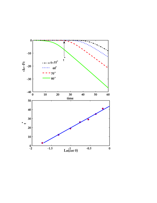
Figure 1: Top plot: evolution of the quantity $v=<h>-Ft$ as a function of time for $\theta=80^{o}$, $70^{o}$, $60^{o}$ and $55^{o}$, and for $\nu=K=0.2$. Bottom plot: the crossover time $t^{*}$ as a function if the incident angle showing the logarithmic dependence of $t^{*}$ on $\mu=cot\theta$.

We integrated equation (2) numerically using Adams-Bashforth scheme Hoffman and imposed periodic boundary conditions. At each time iteration, the function $S$ is determined at each point of the profile, before the height is updated. The initial surface is perturbed with a white noise. The numerical integration of (2) revealed the existence of an incident angle $\theta^{*}$ below which the shadowing effect is irrelevant. This critical angle is mainly determined in the linear regime and is dependent on the ratio $\nu/K$. The smaller this ratio, the larger is the critical angle. Typically, $\theta^{*}$ is in the range 45^o-50^o for $\nu/K$ varying from 10 to 1. To monitor the effect of oblique incidence on growth we followed the evolution of the mean height of the evolving profile, a quantity which is accessible experimentally with the help of scanning probe microscopes. Figure 1 shows the plot of $v=<h>$-$Ft$ versus time( here $<h>$ is the mean height), for $\theta=80^{o}$, $70^{o}$, $60^{o}$ and $55^{o}$, and for $\nu=K=0.2$ and $F=1$. For incident angles larger than the critical angle, one can distinguish two regimes: the first one where $<h>=Ft$ corresponding to the linear regime; the second corresponding to a growth phase where the shadowing influence becomes relevant. This clear distinction identifies a time $t^{*}$ separating the two regimes. For angles smaller than the critical angle, the time $t^{*}$ becomes extremely long and the separation of the linear and the shadowing regimes is no longer clear due to the dominance of the ES non-linearities. In this case, the growth of the surface profile is mainly determined by diffusion and the ES currents since equation (2) is reduced to the well known MBE equation. The time $t^{*}$ can be estimated from geometrical considerations as follows. During the linear regime the typical height is $\sigma$ which is the surface width defined as $\sigma^{2}=\Sigma_{i}\left(h(i)-<h>\right)^{2}\sim\exp({\nu t/l^{2}})$, where $l$ is the typical distance between mounds given by $l=2\pi\sqrt{(2K/\nu)}$Krug02 . If we consider two neighboring mounds of heights $h_{i-1}$ and $h_{i}$ (i is the position on the profile) then the mound $(i-1)$ shadows the mound $i$ when $cot\theta<\frac{h_{i-1}-h_{i}}{l}=\frac{\partial h}{\partial x}\sim\sigma/l$. This gives:

$$t>t^{*}\sim\frac{l^{2}}{\nu}\mbox{ln}(cot\theta)$$ (6)

Figure 1-b shows the logarithmic dependence of $t^{*}$ on $\mu=cot\theta$. The time $t^{*}$ was identified as the time when the quantity $v=<h>-Ft$ drops from zero to negative values as clearly shown in figure 1.

Beyond the time $t^{*}$, nonlinearities caused by shadowing and the ES barrier become significant. Straight after the linear regime and before non-linearities become fully developed, the height $h$ goes through a phase where deep grooves form. This is because valleys become shadowed and stop growing whilst the mound tips continue to grow. At this stage, the ES effect is still weak. As soon as the ES effect starts to be relevant, the deep grooves acquire a mean velocity due to the ES non-linearities, and the grooves morphology disappear, resulting in a morphology dominated by asymmetric mounds or columns at glancing angles. Figure 2 shows an example of the evolution of the profile’s morphology, demonstrating the three phases for the following parameters : $\theta=80^{o}$, $\nu=0.1$, $K=0.2$ and $F=1$. This morphological behavior is true for any $\theta>\theta^{*}$.

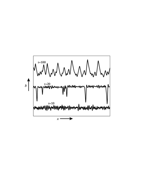
Figure 2: Portion of the evolving profile for three different times: t=10, 20 and 100 for an incident angle of $\theta=80^{o}$. At t=10, the growth is dominated by the linear instability. The intermediate phase (t=20) is characterized by the development of deep grooves on the surface as the shadowing starts to become relevant. Later on (t=100), the deep grooves disappear and the surface settles to a morphology dominated by the ES effect and shadowing, characterized by developing mounds and coarsening. The parameters used here are $\nu=0.2$, $K=0.2$ and $F=1$. The system size was $N=500$.

These observations can be quantified by considering the surface width $\sigma$. In figure 3 the time evolution of this quantity is showing the clear distinction between the above mentioned growth phases. The parameters used here are $\nu=.1$, $K=.2$ and $F=1$. The early time growth is well predicted by the linear theory i.e. $\sigma=\exp(\nu t/l^{2})$. The deep groove phase (indicated by the shaded area in figure 3) induces a sudden increase of the surface width; this phase is followed by a phase where the surface width evolves following a power law e.g. $\sigma\sim t^{\gamma}$.

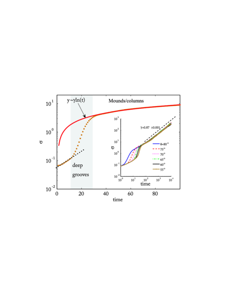
Figure 3: Time evolution of surface width $\sigma$ showing the clear distinction between three growth phases, for an incident angle of $\theta=75^{o}$ and a system size $N=500$. The parameters used here are $\nu=.1$, $K=.2$ and $F=1$. The early time growth is well predicted by the linear theory i.e. $\sigma\sim\exp(\nu t/l^{2})$. The deep groove phase (indicated by the shaded area) induces a sudden increase of the surface width, followed by a growth phase where it evolves following a power law e.g. $\sigma\sim t^{\gamma}$. The inset shows a log-log plot of $\sigma$ vs $t$ for long integration times. The power law exponent $\gamma$ was determined by non-linear regression fit giving a value $\gamma=0.87\pm 0.001$. The result was averaged over 20 realizations.

In the absence of shadowing, the scenario predicted by equation (2) is as follows: after the linear phase where the surface profile undergoes an exponential growth and where mounds form, a coarsening phase develops. During this phase, mounds coarsen and the typical mound size $\lambda$ follows a power law increase in time i.e. $\lambda\sim t^{\beta}$, where $\beta=1/3$Krug02 . In the presence of shadowing, this scenario remains similar. Indeed the coarsening is still persistent but evolves more rapidly than in the absence of shadowing. To show this, we performed long time integration of equation (2) and computed the height autocorrelation function $C(r)=<h(x+r)h(x)>_{x}$. The mounds lateral size $\lambda$ is given by the zero crossing of $C(r)$.

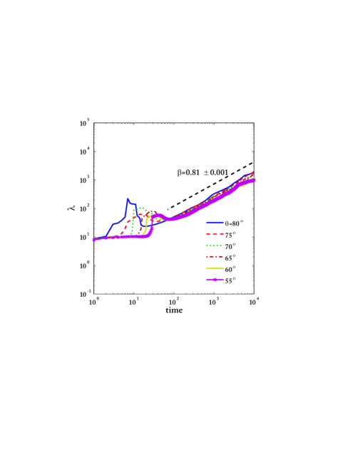
Figure 4: Log-log plot of the mound size $\lambda$ versus time for incident angles $\theta=80^{o}$, $75^{o}$, $70^{o}$, $65^{o}$, $60^{o}$ and $55^{o}$. The power law exponent was determined by regression fit which gives the value of $\beta=0.81\pm 0.001$.

Figure 4 displays a log-log plot of the mounds lateral size versus time for different incident angles. The size of the mounds follows a power law behavior $\lambda\sim t^{\beta}$ with the exponent $\beta=0.81\pm 0.001$. Notice that the value of the exponent is the same for all angles (larger than the critical angle). This tells us the coarsening is faster than in growth in normal incidence where the value of the exponent is 1/3, which is re-confirmed by the integration of equation (2) for angles smaller than $\theta^{*}$.
The draw back of the model (2) is it does not include faceting to account for crystallographic effects and it is restricted to solid-on-solid (SOS) picture. Shim and Amar Amar used kinetic Monte Carlo method which included faceting to simulate homoepitaxial growth of metal(100) under oblique incidence and found that many aspects of the surface morphology can be explained by purely geometrical effects induced by shadowing and demonstrated the appearance of ripples and rods with sides dominated by (111)-oriented facets. Model (2), although it is one dimensional, qualitatively shares some features observed in these simulations; in particular the power law behavior of the surface width and the mounds size as well as the development of asymmetric mounds. In addition, model (2) provided an insight onto the interplay between different growth mechanisms involved in the growth process. Another advantage is that it can simulate long time behavior of the surface morphology without exorbitant computer resources. A natural progression towards simulations which can directly be compared to experimental observations is to extend model (2) to two dimensions. This will have an impact on the experimental design of naturally evolving nanostructures without resorting to expensive lithographic methods such as electron beam lithography.

References

- (1) A. Pimpinelli and J. Villain 1998 Physics of crystal growth (Cambridge University press)
- (2) J. Krug, Physica A 313, 47, (2002).
- (3) G. Ehrlich and F.G. Hudda, J. Chem. Phy. 44, 1039 (1966).
- (4) R. L. Schwoebel, J. Appl. Phys. 40, 614 (1969).
- (5) S. van Dijken, L.C. Jorritsma, and B. Poelsema, Phys. Rev. Lett. 82, 4038 (1999); S. van Dijken, L. C. Jorritsma and B. Poelsema Phys. Rev. B 61, 14047 (2000).
- (6) Y. Shim and J. G. Amar, Phys. Rev. Lett, 98, 046103 (2007).
- (7) R. P. Karunasiri, R. Bruinsma, and J. Rudnick, Phys. Rev. Lett. 62, 788(1989). R. P. Karunasiri, R. Bruinsma, and J. Rudnick, Phys. Rev. Lett. 62, 2767 (1989).
- (8) G. S. Bales, R. Bruinsma, E. A. Eklund, R. P. U. Karunasiri, J. Rudnick and A. Zangwill, Science, 249, 264 (1990).
- (9) P. Politi, G. Grenet, A. Marty, A. Ponchet and J. Villain, Phys. Rep. 324, 271, (2000).
- (10) J. A. Stroscio, D. T. Pierce, M. D. Stiles, A. Zangwill and L. M. Sander, Phys. Rev. Lett. 75, 4246, (1995).
- (11) P. Politi, Phys. Rev. E 58, 281, (1998).
- (12) J. A. Olgilvy, Theory of Wave Scattering from Random Rough Surfaces (Bristol: Institute of Physics Publishing 1991).
- (13) C. Bourlier and G. Berginc, waves in random media, 13, 27, (2003).
- (14) R. J. Wagner, J. Acoust. Soc. Am. 41, 138, (1967). B. G. Smith, IEEE Trans. Antennas Propag. AP-5, 668, (1967).
- (15) R. A. Brokelman and T. Hagfors, IEEE Trans. Antennas Propag.14, 621, (1966).
- (16) Joe D. Hoffman 2001 Numerical Methods for Engineers and Scientists (CRC press)