Field theory of bi- and tetracritical points: Relaxational dynamics

Abstract

We calculate the relaxational dynamical critical behavior of systems of $O(n_{\|})\oplus O(n_{\perp})$ symmetry by renormalization group method within the minimal subtraction scheme in two loop order. The three different bicritical static universality classes previously found for such systems correspond to three different dynamical universality classes within the static borderlines. The Heisenberg and the biconical fixed point lead to strong dynamic scaling whereas in the region of stability of the decoupled fixed point weak dynamic scaling holds. Due to the neighborhood of the stability border between the strong and the weak scaling dynamic fixed point corresponding to the static biconical and the decoupled fixed point a very small dynamic transient exponent, of $\omega_{v}^{{\cal B}}=0.0044$, is present in the dynamics for the physically important case $n_{\|}=1$ and $n_{\perp}=2$ in $d=3$.

I Introduction

The phase diagram of systems with $O(n_{\|})\oplus O(n_{\perp})$ symmetry contains several phases meeting in a multicritical point. In Ref.partI (henceforce called part I) it was shown that the static critical properties can be quantitatively analyzed from field theoretic functions in two loop order if one uses resummation. As an example we have in mind an antiferromagnet in an external magnetic field (with $n_{\|}=1$ and $n_{\perp}=2$), although other physical examples with different values of order parameter (OP) components may be considered.

In order to get more insight in the dynamical critical properties near such a multicritical point we reconsider the simplest dynamical model possible for $O(n_{\|})\oplus O(n_{\perp})$ symmetric systems. In such a dynamical model one assumes relaxational behavior for the two OPs $\vec{\phi}_{\|}$ and $\vec{\phi}_{\perp}$. This model has been briefly studieddohmjanssen77 on the basis of the static one loop results konefi76 . Meanwhilecapevi03 ; Prudnikov98 ; partI it has been shown that the one loop resultskonefi76 ; Lyuksyutov75 are considerably changed in higher loop order concerning the regions of different static multicriticality in the space of OP components $n_{\|}$ and $n_{\perp}$. For integer order parameter components only a system $n_{\|}=1$ and $n_{\perp}=2$ belongs to the universality class characterized by the biconical fixed point (FP) indicating tetracritical behavior - if the physical system lies in the attraction region of the FP.note1

The paper is organized as follows: In chapter II we define the dynamical model, then in chapter III the dynamical field theoretic functions are introduced and the results in two loop order are presented. From these results the FP and dynamical exponents are calculated in chapter IV and the stability of the FP is considered in chapter V. Due to the small dynamic transient exponent found, the effective - nonasymptotic - dynamical behavior is studied in detail in chapter VI. Finally conclusions and an outlook to subsequent research of extended dynamical models is given.

II Dynamical model

The results obtained in part I for the statics of systems with $O(n_{\|})\oplus O(n_{\perp})$ symmetry are applied to the critical dynamics if the system dynamics is described by two relaxational equations for the OP components $\vec{\phi}_{\perp 0}$ and $\vec{\phi}_{\|0}$ in the two subspaces. Correspondingly two kinetic coefficients $\mathring{\Gamma}_{\perp}$ and $\mathring{\Gamma}_{\|}$ have to be introduced. The model A type equations are

$$\frac{\partial\vec{\phi}_{\perp 0}}{\partial t} = -\mathring{\Gamma}_{\perp}\frac{\delta{\mathcal{H}}_{Bi}}{\delta\vec{\phi}_{\perp 0}}+\vec{\theta}_{\phi_{\perp}}\ ,$$ (1)

$$\frac{\partial\vec{\phi}_{\|0}}{\partial t} = -\mathring{\Gamma}_{\|}\frac{\delta{\mathcal{H}}_{Bi}}{\delta\vec{\phi}_{\|0}}+\vec{\theta}_{\phi_{\|}}\,.$$ (2)

The stochastic forces $\vec{\theta}_{\phi_{\perp}}$ and $\vec{\theta}_{\phi_{\|}}$ fulfill Einstein relations

$$\langle\theta_{\phi_{\perp}}^{\alpha}(x,t)\ \theta_{\phi_{\perp}}^{\beta}(x^{\prime},t^{\prime})\rangle\!\!\! = \!\!\!2\mathring{\Gamma}_{\perp}\delta(x-x^{\prime})\delta(t-t^{\prime})\delta^{\alpha\beta}\ ,$$ (3)

$$\langle\theta_{\phi_{\|}}^{i}(x,t)\ \theta_{\phi_{\|}}^{j}(x^{\prime},t^{\prime})\rangle\!\!\! = \!\!\!2\mathring{\Gamma}_{\|}\delta(x-x^{\prime})\delta(t-t^{\prime})\delta^{ij}\ ,$$ (4)

with indices $\alpha,\beta=1,\dots,n_{\perp}$ and $i,j=1,\dots,n_{\|}$ corresponding to the two subspaces. The static functional ${\mathcal{H}}_{Bi}$ is defined as

$${\mathcal{H}}_{Bi}\!=\!\int\!d^{d}x\Bigg{\{}\frac{1}{2}\mathring{r}_{\perp}\vec{\phi}_{\perp 0}\cdot\vec{\phi}_{\perp 0}+\frac{1}{2}\sum_{\alpha=1}^{n_{\perp}}\nabla_{\alpha}\vec{\phi}_{\perp 0}\cdot\nabla_{\alpha}\vec{\phi}_{\perp 0}$$

$$+\frac{1}{2}\mathring{r}_{\|}\vec{\phi}_{\|0}\cdot\vec{\phi}_{\|0}+\frac{1}{2}\sum_{i=1}^{n_{\|}}\nabla_{i}\vec{\phi}_{\|0}\cdot\nabla_{i}\vec{\phi}_{\|0}+\frac{\mathring{u}_{\perp}}{4!}\Big{(}\vec{\phi}_{\perp 0}\cdot\vec{\phi}_{\perp 0}\Big{)}^{2}$$

$$+\frac{\mathring{u}_{\|}}{4!}\Big{(}\vec{\phi}_{\|0}\cdot\vec{\phi}_{\|0}\Big{)}^{2}+\frac{2\mathring{u}_{\times}}{4!}\Big{(}\vec{\phi}_{\perp 0}\cdot\vec{\phi}_{\perp 0}\Big{)}\Big{(}\vec{\phi}_{\|0}\cdot\vec{\phi}_{\|0}\Big{)}\Bigg{\}}\ .$$ (5)

The properties and renormalization of the static vertex functions following from ${\mathcal{H}}_{Bi}$ have already been presented in part I. There in resummed two-loop approximation it has been shown that within a small region in the space of the spatial dimension and the OP components the biconical FP is stable (e.g. for $n_{\|}=1$ and $n_{\perp}=2$ at $d=3$).

III Renormalization, field theoretic functions

From the dynamic equations (1) and (2) a functional may be derived which allows the calculation of dynamic vertex functions in perturbation theory (for an overview see fomorev06 ). Within this dynamic functional additional auxiliary densities $\vec{\tilde{\phi}}_{\perp 0}$ and $\vec{\tilde{\phi}}_{\|0}$ are introducedbauja76 . Recently it has been shown fomo02a that the dynamic two point functions have a general structure, which is in the current model

$$\mathring{\Gamma}_{\phi_{\perp}\tilde{\phi}_{\perp}}\big{(}\xi_{\perp},\xi_{\|},k,\omega\big{)} = -i\omega\mathring{\Omega}_{\phi_{\perp}\tilde{\phi}_{\perp}}\big{(}\xi_{\perp},\xi_{\|},k,\omega\big{)}$$ (6)

$$+\mathring{\Gamma}^{(2,0)}_{\perp\perp}\big{(}\xi_{\perp},\xi_{\|},k\big{)}\mathring{\Gamma}_{\perp}\ ,$$

$$\mathring{\Gamma}_{\phi_{\|}\tilde{\phi}_{\|}}\big{(}\{\xi_{\perp},\xi_{\|},k,\omega\big{)} = -i\omega\mathring{\Omega}_{\phi_{\|}\tilde{\phi}_{\|}}\big{(}\{\xi_{\perp},\xi_{\|},k,\omega\big{)}$$ (7)

$$+\mathring{\Gamma}^{(2,0)}_{\|\|}\big{(}\xi_{\perp},\xi_{\|},k\big{)}\mathring{\Gamma}_{\|}\ ,$$

where $\mathring{\Gamma}^{(2,0)}_{\perp\perp}\big{(}\xi_{\perp},\xi_{\|},k\big{)}$ and $\mathring{\Gamma}^{(2,0)}_{\|\|}\big{(}\xi_{\perp},\xi_{\|},k\big{)}$ are the static two point vertex functions discussed in part I. The functions $\mathring{\Omega}_{\phi_{\perp}\tilde{\phi}_{\perp}}\big{(}\xi_{\perp},\xi_{\|},k,\omega\big{)}$ and $\mathring{\Omega}_{\phi_{\|}\tilde{\phi}_{\|}}\big{(}\xi_{\perp},\xi_{\|},k,\omega\big{)}$ have to be determined within dynamic perturbation expansion. All functions in (6) and (7) depend besides the correlation functions $\xi_{\perp}$, $\xi_{\|}$, the wave vector modulus $k$, and the frequency $\omega$, also on the static couplings $\mathring{u}_{\perp}$, $\mathring{u}_{\times}$ and $\mathring{u}_{\|}$. The functions $\mathring{\Omega}_{\phi_{\alpha_{i}}\tilde{\phi}_{\alpha_{i}}}$ (with $\alpha_{i}=\perp,\|$) additionally depend on the two kinetic coefficients $\mathring{\Gamma}_{\perp}$ and $\mathring{\Gamma}_{\|}$. As we will see below, the genuine representation (6), (7) that allows to single out contributions from merely static vertex functions into dynamic ones essentially simplifies cumbersome calculations and enables one to effectively proceed with calculation of the dynamic RG perturbative expansions.

III.1 Renormalization of the dynamic parameters

The renormalization of the static quantities appearing in (II) has been presented in part I in detail and explicitly performed in the minimal subtraction RG schemeSchloms directly at $d=3$ to the two-loop order. The resulting renormalization factors and field theoretic functions ($\zeta$- and $\beta$-functions) remain valid also in dynamics. Additional renormalizations are necessary for dynamic quantities. Within the current dynamic model only the auxiliary densities and the kinetic coefficients have to be renormalized.

The renormalized counterparts of the auxiliary densities are defined as

$$\vec{\tilde{\phi}}_{\perp 0}=Z_{\tilde{\phi}_{\perp}}^{1/2}\vec{\tilde{\phi}}_{\perp}\ ,\qquad\vec{\tilde{\phi}}_{\|0}=Z_{\tilde{\phi}_{\|}}^{1/2}\vec{\tilde{\phi}}_{\|}\,.$$ (8)

The renormalized kinetic coefficients are introduced as

$$\mathring{\Gamma}_{\perp}=Z_{\Gamma_{\perp}}\Gamma_{\perp}\ ,\qquad\mathring{\Gamma}_{\|}=Z_{\Gamma_{\|}}\Gamma_{\|}\,.$$ (9)

Relation (8) and the renormalization of the OP densities $\vec{\phi}_{\perp 0}$ and $\vec{\phi}_{\|0}$ introduced in part I imply for the dynamic vertex functions the renormalization

$$\Gamma_{\phi_{\perp}\tilde{\phi}_{\perp}} = Z_{\phi_{\perp}}^{1/2}Z_{\tilde{\phi}_{\perp}}^{1/2}\mathring{\Gamma}_{\phi_{\perp}\tilde{\phi}_{\perp}}\ ,$$ (10)

$$\Gamma_{\phi_{\|}\tilde{\phi}_{\|}} = Z_{\phi_{\|}}^{1/2}Z_{\tilde{\phi}_{\|}}^{1/2}\mathring{\Gamma}_{\phi_{\|}\tilde{\phi}_{\|}}\ .$$ (11)

From the above relations and the structure of the dynamic two point vertex functions presented in (6) and (7) follows that the renormalization factors of the kinetic coefficients $\Gamma_{\perp}$ and $\Gamma_{\|}$ in case of the absence of mode couplings are determined by the corresponding renormalization factors of the auxiliary densities. This leads to the relations

$$Z_{\Gamma_{\perp}}=Z_{\phi_{\perp}}^{1/2}Z_{\tilde{\phi}_{\perp}}^{-1/2}\ ,\quad Z_{\Gamma_{\|}}=Z_{\phi_{\|}}^{1/2}Z_{\tilde{\phi}_{\|}}^{-1/2}\,.$$ (12)

The static renormalizaton factors $Z_{\phi_{\perp}}$ and $Z_{\phi_{\|}}$ have been introduced in Eq. (4) of part I.

III.2 Dynamic $\beta$- and $\zeta$-functions in two loop order

Quite analogous to statics in part I we will use the uniform definition

$$\zeta_{a_{i}}(\{u\},\Gamma_{\perp},\Gamma_{\|})=\frac{d\ln Z_{a_{i}}^{-1}}{d\ln\kappa}$$ (13)

for the $\zeta$-functions also in dynamics, where $a_{i}$ is now a placeholder for any auxiliary density or kinetic coefficient, $\kappa$ is the scaling parameter, and $\{u\}=\{u_{\perp},u_{\times},u_{\|}\}$ is the set of static couplings. From perturbation expansion the resulting two loop expressions for the $\zeta$-functions of the kinetic coefficients $\Gamma_{\perp}$ and $\Gamma_{\|}$ read

$$\zeta_{\Gamma_{\perp}} = \frac{n_{\perp}+2}{36}\ u_{\perp}^{2}\left(3\ln\frac{4}{3}-\frac{1}{2}\right)$$

$$+ \frac{n_{\|}}{36}\ u_{\times}^{2}\left[\frac{2}{v}\ln\frac{2(1+v)}{2+v}+\ln\frac{(1+v)^{2}}{v(2+v)}-\frac{1}{2}\right]\,,$$

$$\zeta_{\Gamma_{\|}} = \frac{n_{\|}+2}{36}\ u_{\|}^{2}\left(3\ln\frac{4}{3}-\frac{1}{2}\right)$$

$$+ \frac{n_{\perp}}{36}\ u_{\times}^{2}\left[2v\ln\frac{2(1+v)}{1+2v}+\ln\frac{(1+v)^{2}}{1+2v}-\frac{1}{2}\right]\,.$$

The important dynamic parameter is the time scale ratio

$$v=\frac{\Gamma_{\|}}{\Gamma_{\perp}}$$ (16)

between the two kinetic coefficients $\Gamma_{\perp}$ and $\Gamma_{\|}$, which have been already introduced in (III.2) and (III.2). From the above definition of the time scale ratio and the definition of the $\zeta$-functions in (13) the $\beta$-function of $v$ is determined by

$$\beta_{v}\equiv\kappa\frac{dv}{d\kappa}=v(\zeta_{\Gamma_{\|}}-\zeta_{\Gamma_{\perp}})$$ (17)

where the derivative is taken at fixed unrenormalized quantities. Inserting (III.2) and (III.2) into (17) the two loop expression of the $\beta$-function of $v$ readsdohmjanssen77 ; dohmKFA

$$\beta_{v} = \frac{v}{72}\Bigg{\{}\Big{[}(n_{\|}+2)u_{\|}^{2}-(n_{\perp}+2)u_{\perp}^{2}\Big{]}(6\ln\frac{4}{3}-1)$$

$$- n_{\|}\ u_{\times}^{2}\left[\frac{4}{v}\ln\frac{2(1+v)}{2+v}+2\ln\frac{(1+v)^{2}}{v(2+v)}-1\right]$$

$$+ n_{\perp}\ u_{\times}^{2}\left[4v\ln\frac{2(1+v)}{1+2v}+2\ln\frac{(1+v)^{2}}{1+2v}-1\right]\Bigg{\}}\,.$$

The $\beta$-function changes its sign under interchanging the parallel and perpendicular components and replacing the time scale ratio $v$ by $1/v$.

In the nonasymptotic region where a non universal effective critical behavior may be observed the values of the static couplings and the time scale ratio are described by the flow equations. For $v$ it reads

$$l\frac{dv}{dl}=\beta_{v}\big{(}u_{\|}(l),u_{\perp}(l),u_{\times}(l)\big{)}\,,$$ (19)

whereas for the static couplings Eq. (36) of part I with the Borel resummed static $\beta$-functions are used. The asymptotics is reached in the limit $l\to 0$ starting in the background at $l=1$ from non universal initial values of the time scale ratio and couplings.

IV Fixed points and dynamical critical exponents

As usualfomorev06 the two $\zeta$-functions Eqs. (III.2) and (III.2) define two dynamical critical exponents that govern the power law increase of the autocorrelation time for the OPs $\vec{\phi}_{\|}$ and $\vec{\phi}_{\perp}$, correspondingly

$$z_{\perp}=2+\zeta_{\Gamma_{\perp}}^{\star}\qquad\mbox{and}\qquad z_{\|}=2+\zeta_{\Gamma_{\|}}^{\star}\,,$$ (20)

where the stable FP values of the static and dynamic parameters have been inserted into the $\zeta$-functions, this means $\zeta_{\Gamma_{\alpha_{i}}}^{\star}=\zeta_{\Gamma_{\alpha_{i}}}(\{u^{\star}\},v^{\star})$ . At the strong scaling FP there is only one dynamic time scale and the two exponents are equal whereas at the weak scaling FP they are different and define for each component, parallel and perpendicular, the time scale.

Depending on the FP value of the time scale ratio $v$ one may obtain strong ($v^{\star}\neq 0,\infty$) or weak ($v^{\star}=0,\infty$) dynamic scaling. The dynamical FPs are calculated (see also Eq. (12) in Ref.dohmjanssen77 ) from setting the $\beta$-function (III.2) equal to zero. Inserting the stable static FP values (see Table I in part I) into Eq. (III.2) one then may calculate a dynamical ’phase diagram’ in the $n_{\|}$-$n_{\perp}$-plane quite similar to the static ’phase diagram’ Fig. 1 in part I. Let us note here, that one can make use of two different ways to analyze perturbative expansions within the minimal subtraction RG scheme. The first one is the familiar $\varepsilon$-expansion, when the FP coordinates and asymptotic critical exponents are obtained as series in $\varepsilon=4-d$ and then evaluated at the dimension of interest (e.g. for $d=3$). The second one relies on treatment of the expansions in renormalized couplings directly at fixed dimension $d=3$.Schloms Enhanced by resummation such a scheme allows to treat, besides the asymptotic quantities, the non-universal effective exponents. The latter method has been applied in part I to perform a comprehensive analysis of non-universal static behavior. Below we will make use of the static results obtained there to proceed with the analysis of (asymptotic and effective) dynamical critical behavior.

To summarize an outcome of the static FP stability analysis,konefi76 ; Lyuksyutov75 ; Prudnikov98 ; partI ; capevi03 let us recall that, depending on the $n_{\|}$, $n_{\perp}$ values the critical behavior is governed by one of the three non-trivial FPs: (i) isotropic Heisenberg FP ${\mathcal{H}}(n_{\perp}+n_{\|})$ with $u_{\|}^{\star}=u_{\perp}^{\star}=u_{\times}^{\star}=u^{\star}$; (ii) decoupling FP ${\mathcal{D}}$ with $u_{\|}^{\star}\neq 0,u_{\perp}^{\star}\neq 0,u_{\times}^{\star}=0$; (iii) biconical FP ${\mathcal{B}}$ with $u_{\|}^{\star}\neq 0,u_{\perp}^{\star}\neq 0,u_{\times}^{\star}\neq 0$. Below, we will analyze peculiarities of the dynamical critical behavior in the above universality classes.

IV.1 Dynamics at the isotropic Heisenberg fixed point

At the isotropic Heisenberg FP ${\mathcal{H}}(n_{\perp}+n_{\|})$ the fourth order static couplings are equal, $u_{\|}^{\star}=u_{\perp}^{\star}=u_{\times}^{\star}=u^{\star}$. In consequence the static couplings drop out in the FP equation for $v$. Assuming a nonzero finite value of $v$ at the FP, the equation for $v^{\star}$, $\beta_{v}(v^{\star})=0$, reads

$$0 = \Bigg{\{}\Big{[}(n_{\|}+2)-(n_{\perp}+2)\Big{]}(6\ln\frac{4}{3}-1)$$

$$- n_{\|}\left[\frac{4}{v^{\star}}\ln\frac{2(1+v^{\star})}{2+v^{\star}}+2\ln\frac{(1+v^{\star})^{2}}{v^{\star}(2+v^{\star})}-1\right]$$

$$+ n_{\perp}\left[4v^{\star}\ln\frac{2(1+v^{\star})}{1+2v^{\star}}+2\ln\frac{(1+v^{\star})^{2}}{1+2v^{\star}}-1\right]\Bigg{\}}\,.$$

One immediately sees that for general $n_{\|}$ and $n_{\perp}$ a zero can only be found if the arguments of the logarithms are equal to $4/3$, which leads to the FP value

$$v^{\star}=1\,.$$ (22)

This result has to be fulfilled also in higher loop order and therefore the result is exact. Due to Eq. (22) the $\zeta$-functions (III.2) and (III.2) become equal at the FP

$$\zeta_{\Gamma_{\perp}}^{\star}=\zeta_{\Gamma_{\|}}^{\star}=(n+2)u^{\star}(6\ln\frac{4}{3}-1)$$ (23)

with $n=n_{\|}+n_{\perp}$. This means strong dynamic scaling with the dynamical critical exponent

$$z=2+c\eta$$ (24)

of the $O(n)$-symmetric model A universality class, where $c=6\ln\frac{4}{3}-1$ in two loop order,dyn and $\eta$ is the anomalous dimension of the $O(n)$-symmetric model.

IV.2 Dynamics at the decoupling fixed point

At the decoupling FP ${\mathcal{D}}$ static critical behavior does not fulfill scaling due to the existence of two different correlation lengths, each for one of the decoupled parts of the system (the parallel and perpendicular components of the OP). The FP value of the static coupling $u_{\times}$ is equal to zero. Therefore the flow equation (19) at the static FP reduces to

$$l\frac{dv}{dl}=\frac{v}{72}\Big{(}[(n_{\|}+2)u_{\|}^{\star 2}-(n_{\perp}+2)u_{\perp}^{\star 2}](6\ln\frac{4}{3}-1)\Big{)}$$ (25)

leading either to a flow reaching $v^{\star}=0$ or $1/v^{\star}=0$ depending wether

$$n_{\|}<n_{\perp}\qquad \qquad\zeta_{\Gamma_{\|}}^{\star(A)}<\zeta_{\Gamma_{\perp}}^{\star(A)}\qquad\mbox{or}$$ where

$$n_{\|}>n_{\perp}\qquad \qquad\zeta_{\Gamma_{\|}}^{\star(A)}>\zeta_{\Gamma_{\perp}}^{\star(A)}\,,$$ where (26)

with $\zeta_{\Gamma_{\|,\perp}}^{\star(A)}$ the $\zeta$-function of model A for the corresponding subsystem with $n_{\|,\perp}$ components. Both cases mean that weak scaling holds at the decoupling FP. Indeed inserting the values of the decoupling FP into the $\zeta$-functions (III.2) and (III.2) gives two dynamical exponents $z$. One for the dynamics of the parallel and another for the perpendicular components of the OP. Both exponents correspond to the model A universality class

$$z_{\|}=2+c\eta_{\|}\qquad\mbox{and}\qquad z_{\perp}=2+c\eta_{\perp}\,.$$ (27)

In the special case when $n_{\|}=n_{\perp}$ the exponents $z_{\|}$ and $z_{\perp}$ become equal and the FP values of the time scale ratio are determined by the initial values of the static flow.

IV.3 Dynamics at the biconical fixed point

At the biconical FP ${\mathcal{B}}$ the FP values of the three fourth order couplings are different and the solution for the FP value of $v$ becomes nontrivial and dependent on the number of components $n_{\|}$ and $n_{\perp}$. However the only relevant case where this FP is stable in $d=3$ is $(n_{\|},n_{\perp})=(1,2)$ or $(n_{\|},n_{\perp})=(2,1)$.note1 Due to symmetry the two solutions are related

$$v^{\star}(n_{\|},n_{\perp})=\frac{1}{v^{\star}(n_{\perp},n_{\|})}\,.$$ (28)

The numerical solution found using the static one loop order FP values for the static couplings reads dohmjanssen77

$$v^{\star}(1,2)=v^{{\cal B}}=1.0241.$$ (29)

Thus one finds strong scaling with a new biconical dynamical exponent. Inserting the FP values into the $\zeta$-functions (III.2) and (III.2) the dynamical critical exponent is given by

$$z^{{\cal B}}=2.0149.$$ (30)

As has been shown in part I the biconical FP becomes stable in two loop order within a small region around the OP-component values $n_{\perp}=2$ for $n_{\|}=1$.

Figure 1: Dependence of FP values of the timescale ratio $1/v^{\star}$ and the dynamic transient exponent $\omega_{v}$ on $n_{\perp}$ for $n_{\|}=1$ in the region of stability of the Heisenberg ${\cal H}(3)$ and biconical ${\cal B}$ FP in $d=3$. The dotted vertical line indicates the stability border between ${\cal H}(3)$ and ${\cal B}$. At the stability border to the decoupled FP both $1/v^{\star}$ and $\omega_{v}$ go to zero (at $n_{\perp}\sim 2.18$).

However one has to apply resummation techniques to the two loop functions in order to get real FP values for the static couplings. Using these two loop order resummed values the dependence of the FP value of the time scale ratio $v$ within this region is shown in Fig. 1. Note that we do not resume the expression for $\beta_{v}$, Eq. (III.2), itself. The biconical FP reaches the value of the Heisenberg FP, $v^{{\cal H}(3)}=1$, at the stability border line and the decoupled FP value, $v^{\star}=0$ or $v^{\star}=\infty$ (depending on wether $n_{\|}$ is larger or smaller than $n_{\perp}$) at the corresponding stability border line. Inserting for $n_{\|}=1$ and $n_{\perp}=2$ the resummed FP values for static fourth order couplings into Eq. (III.2) one obtains

$$v^{\star}=v^{{\cal B}}=1.0555.$$ (31)

The corresponding dynamical critical exponent reads

$$z^{{\cal B}}=2.052.$$ (32)

This has to be compared with the predicted value for the Heisenberg FP dohmjanssen77 $z^{{\cal H}(3)}=2.015$, which was found to be stable in the $\epsilon$-expansion in one loop order .

V Dynamic transient exponents

The static stability boundaries are also dynamic stability boundaries and therefore in the case $n_{\|}=1$ and $n_{\perp}=2$ a small dynamic transient exponent is expected. Its value is given by

$$\omega_{v} = \left(\frac{\partial\beta_{v}}{\partial v}\right)_{u_{\times}^{\star},v^{\star}}$$

$$= u_{\times}^{\star 2}\frac{v^{\star}}{18}\bigg{(}\frac{n_{\|}}{v^{\star}}\ln\frac{2(1+v^{\star})}{2+v^{\star}}+n_{\perp}\ln\frac{2(1+v^{\star})}{1+2v^{\star}}\bigg{)}\,.$$

It will be further numerically evaluated by inserting the Borel resummed values for static couplings. As will be shown below this exponent goes to zero only when the dynamical FP changes from the strong dynamic scaling to the weak dynamic scaling FP. This is the case when in addition to the change of the stability of the static FP, the stability of the dynamic FP is changed.

The instability of the weak scaling FP $v^{\star}=0$ or $1/v^{\star}=0$ is defined by a negative dynamic transient exponent

$$\omega_{v} = \left(\frac{\partial\beta_{v}}{\partial v}\right)_{v^{\star}=0}$$ (34)

$$= \frac{1}{72}\Bigg{\{}\Big{[}(n_{\|}+2)u_{\|}^{\star 2}-(n_{\perp}+2)u_{\perp}^{\star 2}\Big{]}(6\ln\frac{4}{3}-1)$$

$$- n_{\|}\ u_{\times}^{\star 2}\left[3-2\lim_{v\to 0}\ln(2v)\right]-n_{\perp}\ u_{\times}^{\star 2}\Bigg{\}}\,.$$

This shows that in any case where $u_{\times}^{\star 2}$ is different from zero the weak scaling FP is never stable. Thus only at the decoupled fixed point the dynamic transient exponent might be positive, if $n_{\|}>n_{\perp}$, see Eq. (IV.2). The transient exponent then reads

$$\omega_{v}=\frac{c}{18}\left(\eta_{\|}-\eta_{\perp}\right)\,.$$ (35)

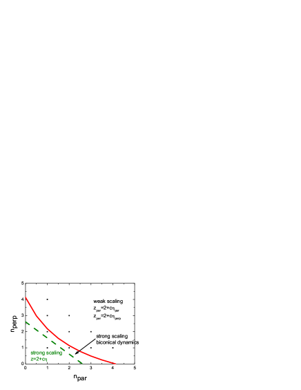
Figure 2: Regions of different static bicritical behavior, which are defined by the stable FP in the $n_{\|}-n_{\perp}$-plane ($\epsilon=4-d=1$) separated by the static stability border lines, (from left to right: Heisenberg FP, biconical FP and decoupled FP). The solid line is also the border line between dynamic strong and weak scaling. The dots indicate small integer values of the component numbers.

At the Heisenberg FP the dynamic transient exponent reduces to

$$\omega_{v}^{{\cal H}}=\frac{n(u^{{\cal H}(n)})^{2}}{18}\ln\frac{4}{3}\,.$$ (36)

Thus the dynamic transient exponent at the stability borderline to the biconical FP is finite and continous (see Fig. 1). In the region of stability of the biconical FP the dynamic transient exponent is given by the expression (V) evaluated with the appropriate FP values for $u_{\times}$ and $v$. At the stability borderlined to the decoupling FP both FP values go to zero. Thus also the dynamic transient exponent goes to zero indicating the change from the stability of the strong scaling dynamic FP to the weak scaling FP. Inserting the FP value for the biconical FP leads to a dynamic transient exponent roughly one order smaller than at the Heisenberg FP due to the smaller FP value of the static coupling $u_{\times}$. Inserting the FP values for the biconical FP into (V) one obtains

$$\omega_{v}^{{\cal B}}=0.0044\,.$$ (37)

Thus in addition to the already small transient from statics an even smaller transient in dynamics appears. This leads to a slow approach of the FP values in the flow equations.

The resulting ’phase diagram’ concerning the dynamical universality classes is shown in Fig. 2. A strong dynamic scaling part at small values for the OP components is separated by a stability border line (solid curve) at which the dynamical transient $\omega_{v}$ goes to zero. This border line lies very near the dot representing the model describing the critical behavior of a three dimensional Heisenberg antiferromagnet in a magnetic field ($n_{\|}=1$, $n_{\perp}=2$). In consequence the transient from the background to the asymptotic behavior might be very slow.

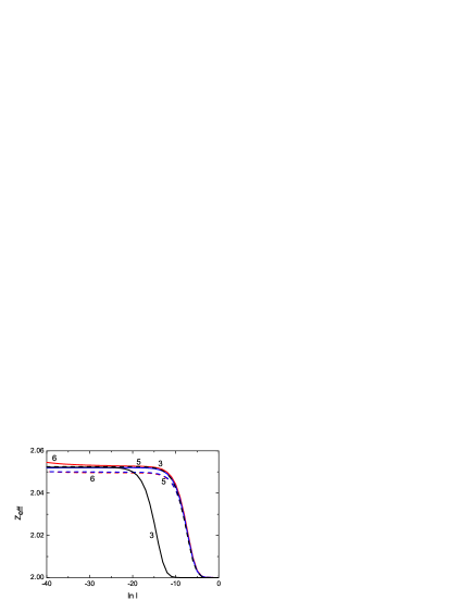
Figure 3: Effective dynamic exponent for the static flows 3, 5 and 6 (see Fig. 1 in part I). The timescale ratio $v$ is set to its biconical FP Eq. (31).

VI Flow equations and effective exponents

The asymptotic dynamic exponents may be reached only in very small region around the FP where the deviation from the FP values in the model parameters have died out. Due to the small transient exponents (either static and/or dynamic) in the physical accessible region the critical behavior may be an effective one described by effective exponents calculated with the parameters different from their FP values at $l=0$ and obtained from the flow equations at finite values of $l$.

Figure 4: Effective dynamic exponent for the static flows 1, 2 and 4 (see Fig. 1 in part I). The timescale ratio $v$ is set to its biconical FP Eq. (31).

The effective exponents are defined as

$$z_{eff,\perp}(l)=2+\zeta_{\Gamma_{\perp}}(u_{\perp}(l),u_{\|}(l),u_{\times}(l),v(l))\,,$$ (38)

$$z_{eff,\|}(l) = 2+\zeta_{\Gamma_{\|}}(u_{\perp}(l),u_{\|}(l),u_{\times}(l),v(l))\,.$$ (39)

In Figs. 3 and 4 we show the effective dynamic exponents for the parallel and perpendicular components of the OP. In the asymptotics when reaching the stable biconical FP both exponents reach the same value since the strong scaling dynamic FP is stable. In order to show the effect of the small static transient exponent we fix the value of the time scale ratio to its biconical FP value. The initial values for the static couplings are chosen to be the same as in part I for the flows in Fig. 1 numbered from 1 to 6. Although the static FP value is not reached (see Fig. 1 in part I) the numerical differences in the effective dynamical exponents are small. The difference between the parallel and perpendicular effective dynamical exponent for curves number 2 and 3 in the background region (larger $l$) result from that part of the static flow where $u_{\times}$ and either $u_{\|}$ or $u_{\perp}$ are almost zero.

In order to show the effect of the smaller dynamical transient exponent (37) we fix the static couplings to their biconical FP values and start the flow for the time scale ratio $v$ at three different initial values corresponding to situation where the parallel relaxation coefficient is smaller, equal or larger to one.

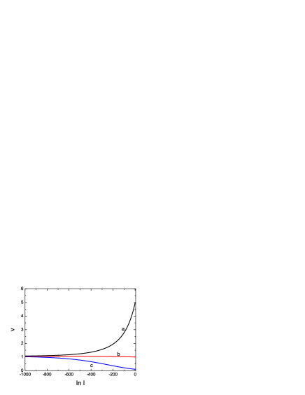
Figure 5: Flows of the timescale ratio $v(l)$ at the biconical static FP ${\cal B}$ for different initial conditions. $v(l=1)=0.1$, $v(l=1)=1$ and $v(l=1)=5$. Note the scale of the flow parameter compared to Figs. 3,4,6.

As one can see from the Fig. 5 indeed for initial values of $v(0)$ far from its FP value, the timescale ratio almost never attains its FP value (for $v(1)=0.1$ it reaches the asymptotics at $\ln\ell\simeq-10^{3}$)! However the effective exponents $z_{eff}$ are not so far from their FP values in consequence of the general dependence on the timescale ratio (see Fig. 6). However one might define a dynamic amplitude ratio from the relaxation rates $\Gamma_{\|}/\Gamma_{\perp}$. This ratio then would in leading order behave like $v$.

Figure 6: Effective dynamical exponents $z_{eff,\|}$ (solid curves) and $z_{eff,\perp}$ (dashed curves) for the flows shown in Fig. 5.

Starting the flows of 3 and 5 with $v$ different from its FP value (see Fig. 7) leads to nonmonotonic behavior of the effective dynamic exponents (see Fig. 8).

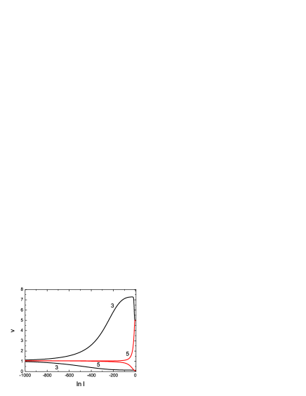
Figure 7: Flows of the timescale ratio $v(l)$ to the biconical static FP ${\cal B}$ for different initial conditions. 3: $v(l=1)=0.1$, 5: $v(l=1)=5$. A quite different behavior is observed.

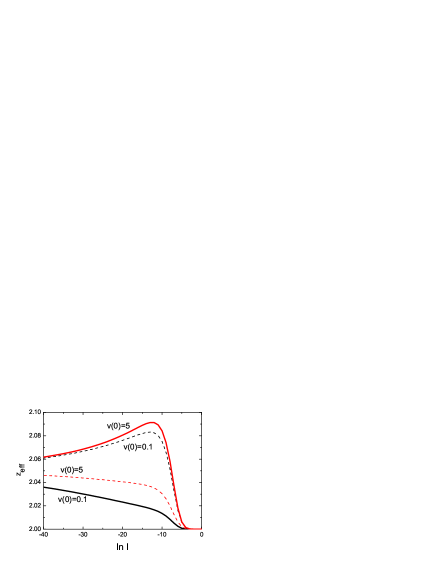
Figure 8: Effective dynamic exponent $z_{eff,\|}$ (solid curves) and $z_{eff,\perp}$ (dashed curves) for the static initial conditions of flow number 5 and dynamic initial conditions as indicated. For the different behavior of the parallel and perpendicular exponent see the text.

At the first sight the behavior of the parallel and perpendicular effective dynamical exponents looks strange since the nonmonotonic behavior is seen in Fig. 8 for small initial values $v(0)$ in the perpendicular exponent, whereas for large values $v(0)$ in the parallel exponent. To explain such an unexpected behavior, one may look at the difference of the two effective exponents (see Eqs (III.2 and III.2)),

$$\Delta z=z_{eff,\|}(u_{\|},u_{\times},u_{\perp},v)-z_{eff,\perp}(u_{\|},u_{\times},u_{\perp},v)$$ (40)

and estimate it at fixed $u_{\|},u_{\times},u_{\perp}$ but for different values of $v$. The difference can be written as:

$$\Delta z=c+\delta z(v).$$ (41)

In Eq. (41), $c$ depends on the static coupling only and $\delta z(v)$ for $n_{\perp}=2$, $n_{\|}=1$ reads:

$$\delta z(v) = \frac{{{\it u_{\times}}}^{2}}{36}\left(4{{\it v}}\,\ln\left(2\,{\frac{1+{\it v}}{1+2{\it v}}}\right)+2\ln\left({\frac{\left(1+{\it v}\right)^{2}}{1+2{\it v}}}\right)\right.$$ (42)

$$- \left.\frac{2}{{{\it v}}}\,\ln\left(2\,{\frac{1+{\it v}}{2+{\it v}}}\right)-\ln\left({\frac{\left(1+{\it v}\right)^{2}}{{\it v}\,\left(2+{\it v}\right)}}\right)\right)$$

depending on $v$ and the static coupling $u_{\times}$. For flows where $u_{\times}$ is very small no difference is seen according to $v$. So no difference is seen in the corresponding flow for the static flow number 3.

However for $u_{\times}$ near the bicritical FP, the difference between $z_{\|}$ and $z_{\perp}$ calculated at the same values of the static couplings but at different values of the timescale ratio sometimes can be positive (i.e. $z_{\|}>z_{\perp}$) and sometimes it can be negative ($z_{\|}<z_{\perp}$), depending on particular values of $v$. Numerically estimates indeed recover the differences shown in Fig. 8

VII Conclusion and outlook

We have reconsidered the relaxational dynamics at the multicritical dynamical FPs in $O(n_{\|})\oplus O(n_{\perp})$ symmetric systems. According to the static two loop order results the biconical FP is the stable FP at the interesting case $n_{\|}=1$ and $n_{\perp}=2$ for which a new dynamic FP with strong dynamic scaling has been found.

The critical dynamics of such a system has to take into account additional properties, namely if the densities of conserved quantities couple statically to the OP and/or if mode coupling term are present. Both extensions of the dynamical equations have to be considered lacking a complete two loop order calculationdohmjanssen77 . The model C like extension of this model will be presented in a third part of this series.

Acknowledgement: This work was supported by the Fonds zur Förderung der wissenschaftlichen Forschung under Project No. P19583-N20.

References

- (1) R. Folk, Y. Holovatch, and G. Moser, submitted to Phys. Rev. 2008; arXiv:0808.0314; henceforth called part I
- (2) V. Dohm and H.-K. Janssen, Phys. Rev. Lett. 39, 946 (1977); J. Appl. Phys. 49, 1347 (1978); see also the review v. Dohm in Multicritical Phenomena, ed. Plenum, New York and London 1983 page 81
- (3) J. M. Kosterlitz, D. Nelson, and M. E. Fisher, Phys. Rev. 13, 412 (1976)
- (4) V. V. Prudnikov, P. V. Prudnikov, and A. A. Fedorenko, JETP Lett. 68, 950 (1998).
- (5) P. Calabrese, A. Pelissetto, and E. Vicari, Phys. Rev. 67, 054505 (2003).
- (6) I. F. Lyuksyutov, V. L. Pokrovskii, and D. E. Khmel nitskii, Sov. Phys. JETP 42, 923 (1975).
- (7) In the minimal subtraction RG scheme at , this result is obtained already in the two-loop approximation, if one properly takes into account the asymptotic propertises of the series obtained.partI It is further supported by the five-loop calculations.capevi03 Noteworthy, a similar analysis of the RG expansions in the massive scheme shows that the two-loop approximation is still insufficient: the biconical FP appears to be stable for , and as well!Prudnikov98 The closeness of the stability borderline between the decoupled FP and the biconical FP to the biconical FP found in Ref.partI is of importance for the effective dynamical behavior as shown in this paper.
- (8) R. Folk and G. Moser, J. Phys. A: Math. Gen. 39, R207 (2006)
- (9) R.Bausch, H.K.Janssen and H.Wagner, Z.Phys.B 24, 113 (1976)
- (10) R. Folk and G. Moser, Phys. Rev. Lett. 89, 125301 (2002)
- (11) V. Dohm, Z. Phys. B 60, 61 (1985); R. Schloms and V. Dohm, Europhys. Lett., 3, 413 (1987); R. Schloms and V. Dohm, Nucl. Phys. B 328, 639 (1989).
- (12) V. Dohm, Report of the Kernforschungsanlage Jülich nr. 1578 (1979)
- (13) B. I. Halperin, P. C. Hohenberg, and S.-k. Ma, Phys. Rev. Lett 29, 1548 (1972)