Balance laws with integrable unbounded sources

Abstract

We consider the Cauchy problem for a $n\times n$ strictly hyperbolic system of balance laws

$$\left\{\begin{array}[]{c}u_{t}+f(u)_{x}=g(x,u),\qquad x\in{\mathbb{R}},t>0\\ u(0,.)=u_{o}\in\mathinner{{{\bf L}^{1}}}\cap\mathinner{\bf BV}({\mathbb{R}};{\mathbb{R}}^{n}),\\ |\lambda_{i}(u)|\geq c>0\mbox{ for all }i\in\{1,\ldots,n\},\\ {\left\|g(x,\cdot)\right\|}_{\mathbf{C}^{2}}\leq\tilde{M}(x)\in\mathinner{{{\bf L}^{1}}},\\ \end{array}\right.$$

each characteristic field being genuinely nonlinear or linearly degenerate. Assuming that the $\mathbf{L}^{1}$ norm of $\|g(x,\cdot)\|_{\mathbf{C}^{1}}$ and $\|u_{o}\|_{\mathinner{\bf BV}({\mathbb{R}})}$ are small enough, we prove the existence and uniqueness of global entropy solutions of bounded total variation extending the result in [1] to unbounded (in $\mathinner{{{\bf L}^{\infty}}}$) sources. Furthermore, we apply this result to the fluid flow in a pipe with discontinuous cross sectional area, showing existence and uniqueness of the underlying semigroup.

2000 Mathematics Subject Classification: 35L65, 35L45, 35L60.

Keywords: Hyperbolic Balance Laws, Unbounded Sources, Pipes with Discontinuous Cross Sections.

1 Introduction

The recent literature offers several results on the properties of gas flows on networks. For instance, in [4, 5, 6, 8] the well posedness is established for the gas flow at a junction of $n$ pipes with constant diameters. The equations governing the gas flow in a pipe with a smooth varying cross section $a(x)$ are given by (see for instance [11]):

$$\left\{\begin{array}[]{l}\frac{\partial\rho}{\partial t}+\frac{\partial q}{\partial x}=-\frac{a^{\prime}(x)}{a(x)}q\\ \frac{\partial q}{\partial t}+\frac{\partial(\frac{q^{2}}{\rho}+p)}{\partial x}=-\frac{a^{\prime}(x)}{a(x)}\frac{q^{2}}{\rho}\\ \frac{\partial e}{\partial t}+\frac{\partial\left(\frac{q}{\rho}(e+p)\right)}{\partial x}=-\frac{a^{\prime}(x)}{a(x)}\left(\frac{q}{\rho}(e+p)\right).\\ \end{array}\right.$$

The well posedness of this system is covered in [1] where an attractive unified approach to the existence and uniqueness theory for quasilinear strictly hyperbolic systems of balance laws is proposed. The case of discontinuous cross sections is considered in the literature inserting a junction with suitable coupling conditions at the junction, see for example [4, 5, 9]. One way to obtain coupling conditions at the point of discontinuity of the cross section $a$ is to take the limit of a sequence of Lipschitz continuous cross sections $a^{\varepsilon}$ converging to $a$ in $\mathinner{{{\bf L}^{1}}}$ (for a different approach see for instance [7]). Unfortunately the results in [1] require $\mathinner{{{\bf L}^{\infty}}}$ bounds on the source term and well posedness is proved on a domain depending on this $\mathinner{{{\bf L}^{\infty}}}$ bound. Since in the previous equations the source term contains the derivative of the cross sectional area one cannot hope to take the limit $a^{\varepsilon}\to a$. Indeed when $a$ is discontinuous, the $\mathinner{{{\bf L}^{\infty}}}$ norm of $(a^{\varepsilon})^{\prime}$ goes to infinity. Therefore the purpose of this paper is to establish the result in [1] without requiring the $\mathinner{{{\bf L}^{\infty}}}$ bound. More precisely, we consider the Cauchy problem for the following $n\times n$ system of equations

$$u_{t}+f(u)_{x}=g(x,u),\qquad x\in{\mathbb{R}},\ t>0,$$ (1)

endowed with a (suitably small) initial data

$$u(0,x)=u_{o}(x),\qquad x\in{\mathbb{R}}.$$ (2)

belonging to $\mathinner{{{\bf L}^{1}}}\cap\mathinner{\bf BV}\left({\mathbb{R}};{\mathbb{R}}^{n}\right)$, the space of integrable functions with bounded total variation (Tot.Var.) in the sense of [12]. Here $u(t,x)\in{\mathbb{R}}^{n}$ is the vector of unknowns, $f:\Omega\to{\mathbb{R}}^{n}$ denotes the fluxes, i.e. a smooth function defined on $\Omega$ which is an open neighborhood of the origin in ${\mathbb{R}}^{n}$. The system (1) is supposed to be strictly hyperbolic, with each characteristic field either genuinely nonlinear or linearly degenerate in the sense of Lax [10]. Concerning the source term $g$, we assume that it satisfies the following Caratheodory–type conditions:

• $g:{\mathbb{R}}\times\Omega\to{\mathbb{R}}^{n}$ is measurable with respect to (w.r.t.) $x$, for any $u\in\Omega$, and is $\mathinner{{{\bf C}^{\bf 2}}}$ w.r.t. $u$, for any $x\in{\mathbb{R}}$;

• there exists a $\mathinner{{{\bf L}^{1}}}$ function $\tilde{M}(x)$ such that ${\left\|g(x,\cdot)\right\|}_{\mathinner{{{\bf C}^{\bf 2}}}}\leq\tilde{M}(x)$;

• there exists a function $\omega\in\mathinner{{{\bf L}^{1}}}({\mathbb{R}})$ such that $\|g(x,\cdot)\|_{\mathinner{{{\bf C}^{\bf 1}}}}\leq\omega(x)$.

Remark 1.

Note that the $\mathinner{{{\bf L}^{1}}}$ norm of $\tilde{M}(x)$ does not have to be small but only bounded differently from $\omega(x)$ whose norm has to be small (see Theorem 1 below). Furthermore condition $(P_{2})$ replaces the $\mathinner{{{\bf L}^{\infty}}}$ bound of the $\mathinner{{{\bf C}^{\bf 2}}}$ norm of $g$ in [1]. Finally observe that we do not require any $\mathinner{{{\bf L}^{\infty}}}$ bound on $\omega$. On the other hand we will need the following observation: if we define

$$\tilde{\varepsilon}_{h}=\sup_{x\in{\mathbb{R}}}\int_{0}^{h}\omega(x+s)\;ds,$$ (3)

by absolute continuity one has $\tilde{\varepsilon}_{h}\to 0$ as $h\to 0$.

Moreover, we assume that a non-resonance condition holds, that is the characteristic speeds of the system (1) are bounded away from zero:

$$|\lambda_{i}(u)|\geq c>0,\qquad\forall~{}u\in\Omega,\ i\in\{1,\ldots,n\}.$$ (4)

The following theorem states the well posedness of (1) in the above defined setting.

Theorem 1.

Assume $(P_{1})$–$(P_{3})$ and (4). If the norm of $\omega$ in $\mathinner{{{\bf L}^{1}}}({\mathbb{R}})$ is sufficiently small, there exist a constant $L>0$, a closed domain ${\cal D}$ of integrable functions with small total variation and a unique semigroup $P:[0,+\infty)\times{\cal D}\rightarrow{\cal D}$ satisfying

1. $P_{0}u=u,\quad P_{t+s}u=P_{t}\circ P_{s}u$ for all $u,v\in{\cal D}$ and $t,s\geq 0$;

2. $\|P_{s}u-P_{t}v\|_{\mathinner{{{\bf L}^{1}}}({\mathbb{R}})}\leq L\Big{(}|s-t|+\|u-v\|_{\mathinner{{{\bf L}^{1}}}({\mathbb{R}})}\Big{)}$ for all $u,v\in{\cal D}$ and $t,s\geq 0$;

3. for all $u_{o}\in{\cal D}$ the function $u(t,\cdot)=P_{t}u_{o}$ is a weak entropy solution of the Cauchy problem (1)–(2) and satisfies the integral estimates (54), (55).

Conversely let $u:[0,T]\rightarrow{\cal D}$ be Lipschitz continuous as a map with values in $\mathinner{{{\bf L}^{1}}}({\mathbb{R}},{\mathbb{R}}^{n})$ and assume that $u(t,x)$ satisfies the integral conditions (54), (55). Then $u(t,\cdot)$ coincides with a trajectory of the semigroup $P$.

The proof of this theorem is postponed to sections 3 and 4, where existence and uniqueness are proved. Before these technical details, we state the application of the above result to gas flow in section 2. Here we apply Theorem 1 to establish the existence and uniqueness of the semigroup related to pipes with discontinuous cross sections. Furthermore, we show that our approach yields the same semigroup as the approach followed in [6] in the special case of two connected pipes. The technical details of section 2 can be found at the end of the paper in section 5.

2 Application to gas dynamics

Theorem 1 provides an existence and uniqueness result for pipes with Lipschitz continuous cross section where the equations governing the gas flow are given by

$$\left\{\begin{array}[]{l}\frac{\partial\rho}{\partial t}+\frac{\partial q}{\partial x}=-\frac{a^{\prime}(x)}{a(x)}q\\ \frac{\partial q}{\partial t}+\frac{\partial(\frac{q^{2}}{\rho}+p)}{\partial x}=-\frac{a^{\prime}(x)}{a(x)}\frac{q^{2}}{\rho}\\ \frac{\partial e}{\partial t}+\frac{\partial\left(\frac{q}{\rho}(e+p)\right)}{\partial x}=-\frac{a^{\prime}(x)}{a(x)}\left(\frac{q}{\rho}(e+p)\right).\end{array}\right.$$ (5)

Here, as usual, $\rho$ denotes the mass density, $q$ the linear momentum, $e$ is the energy density, $a$ is the area of the cross section of the pipe and $p$ is the pressure which is related to the conserved quantities $(\rho,q,e)$ by the equations of state. In most situations, when two pipes of different size have to be connected, the length $l$ of the adaptor is small compared to the length of the pipes. Therefore it is convenient to model these connections as pipes with a jump in the cross sectional area. These discontinuous cross sections however do not fulfill the requirements of Theorem 1. Nevertheless, we can use this Theorem to derive the existence of solutions to the discontinuous problem by a limit procedure. To this end, we approximate the discontinuous function

$$a(x)=\left\{\begin{array}[]{ll}a^{-},&x<0\\ a^{+},&x>0\end{array}\right.$$ (6)

by a sequence $a_{l}\in C^{0,1}({\mathbb{R}},{\mathbb{R}}^{+})$ with the following properties

$$a_{l}(x)=\left\{\begin{array}[]{ll}a^{-},&x<-\frac{l}{2}\\ \varphi_{l}(x),&x\in\left[-\frac{l}{2},\frac{l}{2}\right]\\ a^{+},&x>\frac{l}{2}\end{array}\right.$$ (7)

where $\varphi_{l}$ is any smooth monotone function which connects the two strictly positive constants $a^{-}$, $a^{+}$. One possible choice of the approximations $a_{l}$ as well as the discontinuous pipe with cross section $a$ are shown in figure 1.

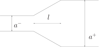
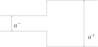
Figure 1: Illustration of approximated and discontinuous cross-sectional area

With the help of Theorem 1 and the techniques used in its proof, we are now able to derive the following Theorem (see also [7] for a similar result obtained with different methods).

Theorem 2.

If $\|a_{l}^{\prime}\|_{\mathinner{{{\bf L}^{1}}}}=|a^{+}-a^{-}|$ is sufficiently small, the semigroups $P^{l}$ related with the smooth section $a_{l}$ converge to a unique semigroup $P$.

The limit semigroup satisfies and is uniquely identified by the integral estimates (54), (55) with $U^{\sharp}$ substituted by $\bar{U}^{\sharp}$ (see Section 5) for the point $\xi=0$. More precisely let $u:[0,T]\rightarrow{\cal D}$ be Lipschitz continuous as a map with values in $\mathinner{{{\bf L}^{1}}}({\mathbb{R}},{\mathbb{R}}^{n})$ and assume that $u(t,x)$ satisfies the integral conditions (54), (55) with $U^{\sharp}$ substituted by $\bar{U}^{\sharp}$ for the point $\xi=0$. Then $u(t,\cdot)$ coincides with a trajectory of the semigroup $P$.

Observe that the same Theorem holds for the $2\times 2$ isentropic system (see Section 5)

$$\left\{\begin{array}[]{l}\frac{\partial\rho}{\partial t}+\frac{\partial q}{\partial x}=-\frac{a^{\prime}(x)}{a(x)}q\\ \frac{\partial q}{\partial t}+\frac{\partial(\frac{q^{2}}{\rho}+p)}{\partial x}=-\frac{a^{\prime}(x)}{a(x)}\frac{q^{2}}{\rho}.\end{array}\right.$$ (8)

In [6] $2\times 2$ homogeneous conservation laws at a junction are considered for given admissible junction conditions. The situation of a junctions with only two pipes with different cross sections can be modeled by our limit procedure or as in [6] with a suitable junction condition. If we define the function $\Psi$ which describes the junction conditions as

$$\Psi\left(\rho_{1},q_{1},\rho_{2},q_{2}\right)=(\rho_{2},q_{2})-\Phi(a^{+}-a^{-},\rho_{1},q_{1})$$ (9)

then it fulfills the determinant condition in [6, Proposition 2.2] since it satisfies Lemma 3. Here $\Phi(a,u)$ is the solution of the ordinary differential equation (72) in Section 5. With these junction conditions one can show that the semigroup obtained in [6] satisfies the same integral estimate (see the following proposition) as our limit semigroup hence they coincide.

Proposition 1.

The semigroup defined in [6] with the junction condition given by (5) satisfies the integral estimates (54), (55) with $U^{\sharp}$ substituted by $\bar{U}^{\sharp}$ for the point $\xi=0$.

The proof is postponed to Section 5.

Remark 2.

Note that Proposition 1 justifies the coupling condition (9) as well as the condition used in [9] to study the Riemann problem for the gas flow through a nozzle.

3 Existence of BV entropy solutions

Throughout the next two sections, we follow the structure of [1]. We recall some definitions and notations in there, and also the results which do not depend on the $\mathinner{{{\bf L}^{\infty}}}$ boundedness of the source term. We will prove only the results which in [1] do depend on the $\mathinner{{{\bf L}^{\infty}}}$ bound using our weaker hypotheses.

3.1 The non homogeneous Riemann-Solver

Consider the stationary equations associated to (1), namely the system of ordinary differential equations:

$$f(v(x))_{x}=g(x,v(x)).$$ (10)

For any $x_{o}\in{\mathbb{R}}$, $v\in\Omega$, consider the initial data

$$v(x_{o})=v.$$ (11)

As in [1], we introduce a suitable approximation of the solutions to (10), (11). Thanks to (4), the map $u\mapsto f(u)$ is invertible inside some neighborhood of the origin; in this neighborhood, for small $h>0$, we can define

$$\Phi_{h}(x_{o},u)\,\dot{=}\,f^{-1}\left[f(u)+\int_{0}^{h}g\left(x_{o}+s,u\right)\,ds\right].$$ (12)

This map gives an approximation of the flow of (10) in the sense that

$$f\left(\Phi_{h}(x_{o},u)\right)-f(u)=\int_{0}^{h}g\left(x_{o}+s,u\right)\,ds.$$ (13)

Throughout the paper we will use the Landau notation ${\cal O}(1)$ to indicate any function whose absolute value remains uniformly bounded, the bound depending only on $f$ and $\|\tilde{M}\|_{\mathinner{{{\bf L}^{1}}}}$.

Lemma 1.

The function $\Phi_{h}(x_{o},u)$ defined in (12) satisfies the following uniform (with respect to $x_{o}\in{\mathbb{R}}$ and to $u$ in a suitable neighborhood of the origin) estimates.

$$\begin{split}&\|\Phi_{h}(x_{o},\cdot)\|_{\mathinner{{{\bf C}^{\bf 2}}}}\leq{\cal O}(1),\qquad\lim_{h\to 0}\sup_{x_{o}\in{\mathbb{R}}}|\Phi_{h}(x_{o},u)-u|=0,\\ &\lim_{h\to 0}\|Id-D_{u}\Phi_{h}(x_{o},u)\|=0\end{split}$$ (14)

Proof.

The Lipschitz continuity of $f^{-1}$ and (3) imply

$$\begin{split}\left|\Phi_{h}(x_{o},u)-u\right|&=\left|\Phi_{h}(x_{o},u)-f^{-1}\left(f(u)\right)\right|\leq{\cal O}(1)\left|\int_{0}^{h}g(x_{o}+s,u)\;ds\right|\\ &\leq{\cal O}(1)\left|\int_{0}^{h}\omega(x_{o}+s)\;ds\right|\leq{\cal O}(1)\tilde{\varepsilon}_{h}\xrightarrow{h\to 0}0.\end{split}$$

Next we compute

$$\begin{split}D_{u}\Phi_{h}(x_{o},u)=&Df^{-1}\left[f(u)+\int_{0}^{h}g(x_{o}+s,u)\;ds\right]\\ &\qquad\cdot\left(Df(u)+\int_{0}^{h}D_{u}g(x_{o}+s,u)\;ds\right)\end{split}$$

which together to the identity $u=f^{-1}\left(f(u)\right)$ implies

$$\begin{split}\left\|D_{u}\Phi_{h}(x_{o},u)-Id\right\|&=\left\|D_{u}\Phi_{h}(x_{o},u)-Df^{-1}\left(f(u\right)\right)\|\\ &\leq\left\|Df^{-1}\left[f(u)+\int_{0}^{h}g(x_{o}+s,u)\;ds\right]-Df^{-1}\left(f(u)\right)\right\|\\ &\qquad\qquad\cdot\left(\|Df(u)\|+\int_{0}^{h}\|D_{u}g(x_{o}+s,u)\|\;ds\right)\\ &\qquad+\left\|Df^{-1}\left(f(u)\right)\right\|\cdot\int_{0}^{h}\|D_{u}g(x_{o}+s,u)\|\;ds\\ &\leq{\cal O}(1)\tilde{\varepsilon}_{h}\xrightarrow{h\to 0}0.\end{split}$$

Finally, denoting with $D_{i}$ the partial derivative with respect to the $i$ component of the state vector and by $\Phi_{h,\ell}$ the $\ell$ component of the vector $\Phi_{h}$, we derive

$$\begin{split}D_{i}D_{j}\Phi_{h,l}(x_{o},u)&=\sum_{k,k^{\prime}}\Bigg{(}D_{k}D_{k^{\prime}}f_{\ell}^{-1}\left(f(u)+\int_{0}^{h}g(x_{o}+s,u)\;ds\right)\\ &\qquad\quad\cdot\left(D_{i}f_{k}(u)+\int_{0}^{h}D_{i}g_{k}(x_{o}+s,u)\;ds\right)\\ &\qquad\quad\cdot\left(D_{j}f_{k^{\prime}}(u)+\int_{0}^{h}D_{j}g_{k^{\prime}}(x_{o}+s,u)\;ds\right)\Bigg{)}\\ &\qquad+\sum_{k}D_{k}f^{-1}_{\ell}\left(f(u)+\int_{0}^{h}g(x_{o}+s,u)\;ds\right)\\ &\qquad\quad\cdot\left(D_{j}D_{i}f_{k}(u)+\int_{0}^{h}D_{j}D_{i}g_{k}(x_{o}+s,u)\;ds\right)\end{split}$$

so that

$$\begin{split}\left\|D^{2}\Phi_{h}(x_{o},u)\right\|&\leq{\cal O}(1)\left(1+\int_{0}^{h}\tilde{M}(x_{o}+s)\;ds\right)\leq{\cal O}(1)\left(1+\|\tilde{M}\|_{\mathinner{{{\bf L}^{1}}}}\right)\leq{\cal O}(1).\end{split}$$

∎

For any $x_{o}\in{\mathbb{R}}$ we consider the system (1), endowed with a Riemann initial datum:

$$u(0,x)=\left\{\begin{array}[]{ll}u_{\ell}&{\rm if}\ x<x_{o}\\ u_{r}&{\rm if}\ x>x_{o}.\end{array}\right.$$ (17)

If the two states $u_{\ell}$, $u_{r}$ are sufficiently close, let $\Psi$ be the unique entropic homogeneous Riemann solver given by the map

$$u_{r}=\Psi({\boldsymbol{\sigma}})(u_{\ell})=\psi_{n}(\sigma_{n})\circ\ldots\circ\psi_{1}(\sigma_{1})(u_{\ell}),$$

where ${\boldsymbol{\sigma}}=(\sigma_{1},\ldots,\sigma_{n})$ denotes the (signed) wave strengths vector in ${\mathbb{R}}^{n}$, [10]. Here $\psi_{j}$, $j=1,\ldots,n$ is the shock–rarefaction curve of the $j^{th}$ family, parametrized as in [3] and related to the homogeneous system of conservation laws

$$u_{t}+f(u)_{x}=0.$$ (18)

Observe that, due to (4), all the simple waves appearing in the solution of (18), (17) propagate with non-zero speed.

To take into account the effects of the source term, we consider a stationary discontinuity across the line $x=x_{o}$, that is, a wave whose speed is equal to 0, the so called zero-wave. Now, given $h>0$, we say that the particular Riemann solution:

$$u(t,x)=\left\{\begin{array}[]{ll}u_{\ell}&{\rm if}\ x<x_{o}\\ u_{r}&{\rm if}\ x>x_{o}.\end{array}\right.\qquad\forall~{}t\geq 0$$ (21)

is admissible if and only if $u_{r}=\Phi_{h}(x_{o},u_{\ell})$, where $\Phi_{h}$ is the map defined in (12). Roughly speaking, we require $u_{\ell}$, $u_{r}$ to be (approximately) connected by a solution of the stationary equations (10).

Definition 1.

Given $h>0$ suitably small, $x_{o}\in{\mathbb{R}}$, we say that $u(t,x)$ is a $h$–Riemann solver for (1), (4), (17), if the following conditions hold

• there exist two states $u^{-}$, $u^{+}$ which satisfy $u^{+}=\Phi_{h}(x_{o},u^{-})$;

• on the set $\{t\geq 0,\ x<x_{o}\}$, $u(t,x)$ coincides with the solution to the homogeneous Riemann Problem (18) with initial values $u_{\ell}$, $u^{-}$ and, on the set $\{t\geq 0,\ x>x_{o}\}$, with the solution to the homogeneous Riemann Problem with initial values $u^{+}$, $u_{r}$;

• the Riemann Problem between $u_{\ell}$ and $u^{-}$ is solved only by waves with negative speed (i.e. of the families $1,\ldots,p$);

• the Riemann Problem between $u^{+}$ and $u_{r}$ is solved only by waves with positive speed (i.e. of the families $p+1,\ldots,n$).

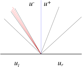
Figure 2: Wave structure in an $h$–Riemann solver.

Lemma 2.

Let $x_{o}\in{\mathbb{R}}$ and $u,\ u_{1},\ u_{2}$ be three states in a suitable neighborhood of the origin. For $h$ suitably small, one has

$$\left|\Phi_{h}(x_{o},u)-u\right| = {\cal O}(1)\int_{0}^{h}\omega(x_{o}+s)\;ds,$$ (22)

$$\left|\Phi_{h}(x_{o},u_{2})-\Phi_{h}(x_{o},u_{1})-(u_{2}-u_{1})\right| = {\cal O}(1)|u_{2}-u_{1}|\int_{x_{o}}^{x_{o}+h}\omega(s)ds.$$ (23)

Lemma 3.

For any $M>0$ there exist ${\delta}_{1}^{\prime},\ h_{1}^{\prime}>0$, depending only on $M$ and the homogeneous system (18), such that the following holds. For all maps $\phi\in\mathinner{{{\bf C}^{\bf 2}}}({\mathbb{R}}^{n},{\mathbb{R}}^{n})$ satisfying

$$\|\phi\|_{\mathinner{{{\bf C}^{\bf 2}}}}\leq M,\qquad|\phi(u)-u|\leq h_{1}^{\prime},\qquad\|I-D\phi(u)\|\leq h_{1}^{\prime}$$

and for all $u_{\ell}\in B(0,{\delta}_{1}^{\prime})$, $u_{r}\in B(\phi(0),{\delta}_{1}^{\prime})$ there exist $n+1$ states $w_{0},\ldots,w_{n+1}$ and $n$ wave sizes $\sigma_{1},\ldots,\sigma_{n}$, depending smoothly on $u_{\ell},\ u_{r}$, such that with previous notations:

1. $w_{0}=u_{\ell},\ w_{n+1}=u_{r}$;

2. $w_{i}=\Psi_{i}(\sigma_{i})(w_{i-1}),\qquad i=1,\ldots,p$;

3. $w_{p+1}=\phi(w_{p})$;

4. $w_{i+1}=\Psi_{i}(\sigma_{i})(w_{i}),\qquad i=p+1,\ldots,n$.

The next lemma establishes existence and uniqueness for the $h$–Riemann solvers (see Fig.2).

Lemma 4.

There exist ${\delta}_{1},\ h_{1}>0$ such that the following holds: for any $x_{o}\in{\mathbb{R}}$, $h\in[0,h_{1}]$, $u_{\ell}$, $u_{r}\in B(0,{\delta}_{1})$, there exists a unique $h$–Riemann solver in the sense of Definition 1.

Proof.

By Lemma 1 if $h_{1}>0$ is chosen sufficiently small then for any $h\in[0,h_{1}]$, $x_{o}\in{\mathbb{R}}$ the map $u\mapsto\Phi_{h}(x_{o},u)$ meets the hypotheses of Lemma 3. Finally taking $h_{1}$ eventually smaller we can obtain that there exists ${\delta}_{1}>0$ such that $B(0,{\delta}_{1})\subset B(0,{\delta}_{1}^{\prime})\cap B(\Phi_{h}(x_{o},0),{\delta}_{1}^{\prime})$, for any $h\in[0,h_{1}]$. ∎

In the sequel, $E$ stands for the implicit function given by Lemmas 3 and 4:

$${\boldsymbol{\sigma}}\dot{=}E(h,u_{\ell},u_{r};x_{o}),$$

which plays the role of a wave–size vector. We recall that, by Lemma 3, $E$ is a $\mathinner{{{\bf C}^{\bf 2}}}$ function with respect to the variables $u_{\ell},u_{r}$ and its $\mathinner{{{\bf C}^{\bf 2}}}$ norm is bounded by a constant independent of $h$ and $x_{o}$.

In contrast with the homogeneous case, the wave–size ${\boldsymbol{\sigma}}$ in the $h$–Riemann solver is not equivalent to the jump size $|u_{\ell}-u_{r}|$; an additional term appears coming from the “Dirac source term” (see the special case $u_{\ell}=u_{r}$).

Lemma 5.

Let ${\delta}_{1},\ h_{1}$ be the constants in Lemma 4. For $u_{\ell},u_{r}\in B(0,{\delta}_{1})$, $h\in[0,h_{1}]$, set ${\boldsymbol{\sigma}}=E[h,u_{\ell},u_{r};x_{o}]$. Then it holds:

$$\begin{array}[]{rcl}|u_{\ell}-u_{r}|&=&{\cal O}(1)\left(|{\boldsymbol{\sigma}}|+\displaystyle{\int_{0}^{h}\omega(x_{o}+s)\;ds}\right),\\ |{\boldsymbol{\sigma}}|&=&{\cal O}(1)\left(|u_{\ell}-u_{r}|+\displaystyle{\int_{0}^{h}\omega(x_{o}+s)\;ds}\right).\end{array}$$ (26)

3.2 Existence of a Lipschitz semigroup of $\mathinner{\bf BV}$ entropy solutions

Note that as shown in [1] we can identify the sizes of the zero waves with the quantity

$$\sigma=\int_{0}^{h}\omega(jh+s)\,ds.$$ (27)

With this definition all the Glimm interaction estimates continue to hold with constants that depend only on $f$ and on $\|\tilde{M}\|_{\mathinner{{{\bf L}^{1}}}}$, therefore all the wave front tracking algorithm can be carried out obtaining the existence of $\varepsilon,h$-approximate solutions as defined below.

Definition 2.

Given $\epsilon,h>0$, we say that a continuous map

$$u^{\epsilon,h}:[0,+\infty)\rightarrow\mathinner{{{\bf L}^{1}}}_{loc}\left({\mathbb{R}},{\mathbb{R}}^{n}\right)$$

is an $\epsilon,h$–approximate solution of (1)–(2) if the following holds:

• As a function of two variables, $u^{\epsilon,h}$ is piecewise constant with discontinuities occurring along finitely many straight lines in the $x,t$ plane. Only finitely many wave-front interactions occur, each involving exactly two wave-fronts, and jumps can be of four types: shocks (or contact discontinuities), rarefaction waves, non-physical waves and zero-waves: ${\cal J}={\cal S}\cup{\cal R}\cup{\cal NP}\cup{\cal Z}$.

• Along each shock (or contact discontinuity) $x_{\alpha}=x_{\alpha}(t)$, $\alpha\in{\cal S}$, the values of $u^{-}=u^{\epsilon,h}(t,x_{\alpha}-)$ and $u^{+}=u^{\epsilon,h}(t,x_{\alpha}+)$ are related by $u^{+}=\psi_{{k_{\alpha}}}(\sigma_{\alpha})(u^{-})$ for some ${k_{\alpha}}\in\{1,...,n\}$ and some wave-strength $\sigma_{\alpha}$. If the ${k_{\alpha}}^{th}$ family is genuinely nonlinear, then the Lax entropy admissibility condition $\sigma_{\alpha}<0$ also holds. Moreover, one has

  $$|\dot{x}_{\alpha}-\lambda_{{k_{\alpha}}}(u^{+},u^{-})|\leq\epsilon$$

  where $\lambda_{{k_{\alpha}}}(u^{+},u^{-})$ is the speed of the shock front (or contact discontinuity) prescribed by the classical Rankine-Hugoniot conditions.

• Along each rarefaction front $x_{\alpha}=x_{\alpha}(t)$, $\alpha\in{\cal R}$, one has $u^{+}=\psi_{{k_{\alpha}}}(\sigma_{\alpha})(u^{-})$, $0<\sigma_{\alpha}\leq\epsilon$ for some genuinely nonlinear family ${k_{\alpha}}$. Moreover, we have: $|\dot{x}_{\alpha}-\lambda_{{k_{\alpha}}}(u^{+})|\leq\epsilon$.

• All non-physical fronts $x=x_{\alpha}(t)$, $\alpha\in{\cal NP}$ travel at the same speed $\dot{x}_{\alpha}=\hat{\lambda}>\sup_{u,i}|\lambda_{i}(u)|$. Their total strength remains uniformly small, namely:

  $$\sum_{\alpha\in{\cal NP}}|u^{\epsilon,h}(t,x_{\alpha}+)-u^{\epsilon,h}(t,x_{\alpha}-)|\leq\epsilon,\qquad\forall~{}t>0.$$

• The zero-waves are located at every point $x=jh$, $j\in(-\frac{1}{h\epsilon},\frac{1}{h\epsilon})\cap{\mathbb{Z}}$.
  Along a zero-wave located at $x_{\alpha}=j_{\alpha}h$, $\alpha\in{\cal Z}$, the values $u^{-}=u^{\epsilon,h}(t,x_{\alpha}-)$ and $u^{+}=u^{\epsilon,h}(t,x_{\alpha}+)$ satisfy $u^{+}=\Phi_{h}(x_{\alpha},u^{-})$ for all $t>0$ except at the interaction points.

• The total variation in space $\mathop{\mbox{\rm Tot.Var.}}u^{\epsilon,h}(t,\cdot)$ is uniformly bounded for all $t\geq 0$. The total variation in time $\mathop{\mbox{\rm Tot.Var.}}\left\{u^{\epsilon,h}(\cdot,x);[0,+\infty)\right\}$ is uniformly bounded for $x\not=jh$, $j\in{\mathbb{Z}}$.

Finally, we require that $\|u^{\epsilon,h}(0,.)-u_{o}\|_{\mathinner{{{\bf L}^{1}}}({\mathbb{R}})}\leq\epsilon$.

Keeping $h>0$ fixed, we are about to let first $\epsilon$ tend to zero. Hence we shall drop the superscript $h$ for notational clarity.

Theorem 3.

Let $u^{\epsilon}$ be a family of $\epsilon,h$–approximate solutions of (1)–(2). There exists a subsequence $u^{\epsilon_{i}}$ converging as $i\rightarrow+\infty$ in ${\bf L}^{1}_{loc}\left((0,+\infty)\times{\mathbb{R}}\right)$ to a function $u$ which satisfies for any $\varphi\in{\bf C}^{1}_{c}\left((0,+\infty)\times{\mathbb{R}}\right)$:

$$\int_{0}^{\infty}\int_{\mathbb{R}}\left[u\varphi_{t}+f(u)\varphi_{x}\right]dxdt$$

$$+\int_{0}^{\infty}\sum_{j\in{\mathbb{Z}}}\varphi(t,jh)\left(\int_{0}^{h}g\left[jh+s,u(t,jh-)\right]ds\right)dt=0.$$ (28)

Moreover $\mathop{\mbox{\rm Tot.Var.}}u(t,\cdot)$ is uniformly bounded and $u$ satisfies the Lipschitz property

$$\int_{\mathbb{R}}\left|u(t^{\prime},x)-u(t^{\prime\prime},x)\right|dx\leq C^{\prime}|t^{\prime}-t^{\prime\prime}|,\qquad t^{\prime},t^{\prime\prime}\geq 0;$$ (29)

Now we are in position to prove [1, Theorem 4] with our weaker hypotheses. As in [1] we can apply Helly’s compactness theorem to get a subsequence $u^{h_{i}}$ converging to some function $u$ in $\mathinner{{{\bf L}^{1}}}_{loc}$ whose total variation in space is uniformly bounded for all $t\geq 0$. Moreover, working as in [2, Proposition 5.1], one can prove that $u^{h_{i}}(t,\cdot)$ converges in $\mathinner{{{\bf L}^{1}}}$ to $u(t,\cdot)$, for all $t\geq 0$.

Theorem 4.

Let $u^{h_{i}}$ be a subsequence of solutions of equation (28) with uniformly bounded total variation converging as $i\rightarrow+\infty$ in $\mathinner{{{\bf L}^{1}}}$ to some function $u$. Then $u$ is a weak solution to the Cauchy problem (1)–(2).

We omit the proofs of Theorem 3 and 4 since they are very similar to the proofs of [1, Theorem 3 and 4]. We only observe that, in those proofs, the computations which rely on the $\mathinner{{{\bf L}^{\infty}}}$ bound on the source term have to be substituted by the following estimates.

• Concerning the proof of Theorem 3:

  $$\begin{split}&\int_{0}^{h}\left|g\left(jh+s,u^{\varepsilon}(t,jh-)\right)-g\left(jh+s,u(t,jh-)\right)\right|\;ds\\ &\qquad\leq\int_{0}^{h}\left\|g(jh+s,\cdot)\right\|_{\mathinner{{{\bf C}^{\bf 1}}}}\cdot\left|u^{\varepsilon}(t,jh-)-u(t,jh-)\right|\;ds\\ &\qquad\leq\tilde{\varepsilon}_{h}\cdot\left|u^{\varepsilon}(t,jh-)-u(t,jh-)\right|.\end{split}$$

• Concerning the proof of Theorem 4:

  $$\begin{split}&\int_{0}^{h}\left|g\left(jh+s,u^{h}(t,jh-)\right)\right|\;ds\leq\int_{0}^{h}\left\|g(jh+s,\cdot)\right\|_{\mathinner{{{\bf C}^{\bf 1}}}}\;ds\leq\tilde{\varepsilon}_{h}\end{split}$$

  and

  $$\begin{split}&\int_{0}^{h}\left|g\left(jh+s,u^{h}(t,jh-)\right)-g\left(jh+s,u(t,jh+s)\right)\right|\;ds\\ &\qquad\leq\int_{0}^{h}\left\|g(jh+s,\cdot)\right\|_{\mathinner{{{\bf C}^{\bf 1}}}}\cdot\left|u^{h}(t,jh-)-u(t,jh+s)\right|\;ds\\ &\qquad\leq\tilde{\varepsilon}_{h}\cdot\mathop{\mbox{\rm Tot.Var.}}\left\{u^{h}(t,\cdot),[(j-1)h,(j+1)h]\right\}\\ &\qquad\quad+\int_{jh}^{(j+1)h}\omega(x)\left|u^{h}(t,x)-u(t,x)\right|.\end{split}$$

We observe that all the computations done in [1, Section 4] rely on the source $g$ only through the amplitude of the zero waves and on the interaction estimates. Therefore the following two theorems still hold in the more general setting.

Theorem 5.

There exists ${\delta}>0$ such that if $\left\|\omega\right\|_{\mathinner{{{\bf L}^{1}}}({\mathbb{R}})}$ is sufficiently small, then for any (small) $h>0$ there exist a non empty closed domain ${\cal D}_{h}({\delta})$ and a unique uniformly Lipschitz semigroup $P^{h}:[0,+\infty)\times{\cal D}_{h}({\delta})\rightarrow{\cal D}_{h}({\delta})$ whose trajectories $u(t,.)=P_{t}^{h}u_{o}$ solve (28) and are obtained as limit of any sequence of $\epsilon,h$–approximate solutions as $\epsilon$ tends to zero with fixed $h$. In particular the semigroups $P^{h}$ satisfy for any $u_{o},v_{o}\in{\cal D}_{h}({\delta})$, $t,s\geq 0$

$$P^{h}_{0}u_{o}=u_{o},\qquad P^{h}_{t}\circ P^{h}_{s}u_{o}=P^{h}_{s+t}u_{o},$$ (30)

$$\left\|P^{h}_{t}u_{o}-P^{h}_{s}v_{o}\right\|_{\mathinner{{{\bf L}^{1}}}({\mathbb{R}})}\leq L\left[\left\|u_{o}-v_{o}\right\|_{\mathinner{{{\bf L}^{1}}}({\mathbb{R}})}+|t-s|\right]$$ (31)

for some $L>0$, independent on $h$.

Theorem 6.

If $\left\|\omega\right\|_{\mathinner{{{\bf L}^{1}}}({\mathbb{R}})}$ is sufficiently small, there exist a constant $L>0$, a non empty closed domain ${\cal D}$ of integrable functions with small total variation and a semigroup $P:[0,+\infty)\times{\cal D}\rightarrow{\cal D}$ with the following properties

1. $P_{0}u=u,\quad\forall u\in{\cal D};\qquad P_{t+s}u=P_{t}\circ P_{s}u,\quad\forall u\in{\cal D},\ t,s\geq 0.$

2. $\|P_{s}u-P_{t}v\|_{\mathinner{{{\bf L}^{1}}}({\mathbb{R}})}\leq L\Big{(}|s-t|+\|u-v\|_{\mathinner{{{\bf L}^{1}}}({\mathbb{R}})}\Big{)},\quad\forall u\in{\cal D},\ t,s\geq 0.$

3. for all $u_{o}\in{\cal D}$, the function $u(t,\cdot)=P_{t}u_{o}$ is a weak entropy solution of system (1).

4. for some ${\delta}>0$ and all $h>0$ small enough ${\cal D}\subset{\cal D}_{h}({\delta})$.

5. There exists a sequence of semigroups $P^{h_{i}}$ such that $P^{h_{i}}_{t}u$ converges in $\mathinner{{{\bf L}^{1}}}$ to $P_{t}u$ as $i\rightarrow+\infty$ for any $u\in{\cal D}$.

Remark 3.

Looking at [1, (4.6)] and the proof of [1, Theorem 7] one realizes that the invariant domains $\mathcal{D}_{h}(\delta)$ and $\mathcal{D}$ depend on the particular source term $g(x,u)$. On the other hand estimate [1, (4.4)] shows that all these domains contain all integrable functions with sufficiently small total variation. Since the bounds ${\cal O}(1)$ in Lemma 5 depend only on $f$ and on $\|\tilde{M}\|_{\mathinner{{{\bf L}^{1}}}}$, also the constant $C_{1}$ in [1, (4.4)] depends only on $f$ and on $\|\tilde{M}\|_{\mathinner{{{\bf L}^{1}}}}$. Therefore there exists $\tilde{\delta}>0$ depending only on $f$ and on $\|\tilde{M}\|_{\mathinner{{{\bf L}^{1}}}}$ such that $\mathcal{D}_{h}(\delta)$ and $\mathcal{D}$ contain all integrable functions $u(x)$ with $\mathop{\mbox{\rm Tot.Var.}}\left\{u\right\}\leq\tilde{\delta}$.

4 Uniqueness of $\mathinner{\bf BV}$ entropy solutions

The proof of uniqueness in [1] strongly depends on the boundedness of the source, therefore we have to consider it in a more careful way.

4.1 Some preliminary results

As in [1] we shall make use of the following technical lemmas whose proofs can be found in [3].

Lemma 6.

Let $(a,b)$ a (possibly unbounded) open interval, and let $\hat{\lambda}$ be an upper bound for all wave speeds. If $\bar{u},\ \bar{v}\in{\cal D}_{h}({\delta})$ then for all $t\geq 0$ and $h>0$, one has

$$\int_{a+\hat{\lambda}t}^{b-\hat{\lambda}t}\left|\left(P^{h}_{t}\bar{u}\right)(x)-\left(P^{h}_{t}\bar{v}\right)(x)\right|dx\leq L\int_{a}^{b}\left|\bar{u}(x)-\bar{v}(x)\right|dx.$$ (32)

Lemma 7.

Given any interval $I_{0}=[a,b]$, define the interval of determinacy

$$I_{t}=[a+\hat{\lambda}t,b-\hat{\lambda}t],\qquad t<\frac{b-a}{2\hat{\lambda}}.$$ (33)

For every Lipschitz continuous map $w:[0,T]\mapsto{\cal D}_{h}({\delta})$ and $h>0$:

$$\left\|w(t)-P^{h}_{t}w(0)\right\|_{\mathinner{{{\bf L}^{1}}}(I_{t})}$$

$$\leq L\int_{0}^{t}\left\{\liminf_{\eta\rightarrow 0}\frac{\left\|w(s+\eta)-P^{h}_{\eta}w(s)\right\|_{\mathinner{{{\bf L}^{1}}}(I_{s+\eta})}}{\eta}\right\}ds.$$

Remark 4.

Lemmas 6, 7 hold also substituting $P^{h}$ with the operator $P$. In this case we have obviously to substitute the domains ${\cal D}_{h}({\delta})$ with the domain ${\cal D}$ of Theorem 6.

Let now $u_{\ell},u_{r}$ be two nearby states and $\lambda<\hat{\lambda}$; we consider the function

$$v(t,x)=\left\{\begin{array}[]{lll}u_{\ell}&\mbox{ if }&x<\lambda t+x_{o}\\ u_{r}&\mbox{ if }&x\geq\lambda t+x_{o}.\end{array}\right.$$ (37)

Lemma 8.

Call $w(t,x)$ the self-similar solution given by the standard homogeneous Riemann Solver with the Riemann data (17).

1. In the general case, one has

   $$\frac{1}{t}\int_{-\infty}^{+\infty}\left|v(t,x)-w(t,x)\right|dx={\cal O}(1)|u_{\ell}-u_{r}|;$$ (38)

2. Assuming the additional relations $u_{r}=R_{i}(\sigma)(u_{\ell})$ and $\lambda=\lambda_{i}(u_{r})$ for some $\sigma>0$, $i=1,\ldots,n$ one has the sharper estimate

   $$\frac{1}{t}\int_{-\infty}^{+\infty}\left|v(t,x)-w(t,x)\right|dx={\cal O}(1)\sigma^{2};$$ (39)

3. Let $u^{*}\in\Omega$ and call $\lambda_{1}^{*}<\ldots<\lambda_{n}^{*}$ the eigenvalues of the matrix $A^{*}=\nabla f(u^{*})$. If for some $i$ it holds $A^{*}(u_{r}-u_{\ell})=\lambda_{i}^{*}(u_{r}-u_{\ell})$ and $\lambda=\lambda_{i}^{*}$ in (37) then one has

   $$\frac{1}{t}\int_{-\infty}^{+\infty}\left|v(t,x)-w(t,x)\right|dx={\cal O}(1)|u_{\ell}-u_{r}|\Big{(}|u_{\ell}-u^{*}|+|u^{*}-u_{r}|\Big{)};$$ (40)

We now prove the next result which is directly related to our $h$-Riemann solver.

Lemma 9.

Call $w(t,x)$ the self-similar solution given by the $h$–Riemann Solver in $x_{o}$ with the Riemann data (17).

1. In the general case one has

   $$\frac{1}{t}\int_{-\infty}^{+\infty}\left|v(t,x)-w(t,x)\right|dx={\cal O}(1)\Big{(}|u_{\ell}-u_{r}|+\int_{0}^{h}\omega(x_{o}+s)\;ds\Big{)};$$ (41)

2. Assuming the additional relation

   $$u_{r}=u_{\ell}+\left[\nabla f\right]^{-1}(u^{*})\displaystyle{\int_{0}^{h}}g(x_{o}+s,u^{*})ds$$

   with $\lambda=0$ in (37) one has the sharper estimate

   $$\frac{1}{t}\int_{-\infty}^{+\infty}\left|v(t,x)-w(t,x)\right|dx$$ (42)

   $$= {\cal O}(1)\Big{(}\int_{0}^{h}\omega(x_{o}+s)\;ds+|u_{\ell}-u^{*}|\Big{)}\cdot\int_{0}^{h}\omega(x_{o}+s)\;ds.$$

Proof. Estimate (i) is a direct consequence of Lemma 5. Let us prove now (ii). Since $\lambda=0$ we derive

$$\frac{1}{t}\int_{-\infty}^{+\infty}\left|v(t,x)-w(t,x)\right|dx$$

$$= \frac{1}{t}\int_{-\hat{\lambda}t}^{0}\left|u_{\ell}-w(t,x)\right|dx+\frac{1}{t}\int_{0}^{\hat{\lambda}t}\left|u_{r}-w(t,x)\right|dx$$

$$= {\cal O}(1)\left[\sum_{\iota=1}^{p}|\sigma_{\iota}|+\sum_{\iota=p+1}^{n}|\sigma_{\iota}|\right]={\cal O}(1)|{\boldsymbol{\sigma}}|.$$

This leads to

$$|{\boldsymbol{\sigma}}| = \Big{|}E\left[h,u_{\ell},u_{r};x_{o}\right]-E\left[h,u_{\ell},\Phi_{h}(x_{o},u_{\ell});x_{o}\right]\Big{|}$$

$$= {\cal O}(1)\left|u_{r}-\Phi_{h}(x_{o},u_{\ell})\right|.$$

To estimate this last term, we define $b(y,u)=f^{-1}\left(f(u)+y\right)$ and compute for some $y_{1},\;y_{2}$:

$$\left|u_{\ell}+\left[\nabla f\right]^{-1}(u^{*})y_{1}-b(y_{2},u_{\ell})\right| \leq {\cal O}(1)|y_{1}|\cdot|u^{*}-u_{\ell}|+{\cal O}(1)|y_{1}-y_{2}|$$

$$+\left|u_{\ell}+\left[\nabla f\right]^{-1}(u_{\ell})y_{2}-b\left(y_{2},u_{\ell}\right)\right|.$$

The function $z(y_{2})=u_{\ell}+\left[\nabla f\right]^{-1}(u_{\ell})y_{2}-b\left(y_{2},u_{\ell}\right)$ satisfies $z(0)=0$, $D_{y_{2}}z(0)=0$, hence we have the estimate

$$\left|u_{\ell}+\left[\nabla f\right]^{-1}(u^{*})y_{1}-b(y_{2},u_{\ell})\right|\leq{\cal O}(1)\left[|y_{1}|\cdot|u^{*}-u_{\ell}|+|y_{1}-y_{2}|+\left|y_{2}\right|^{2}\right].$$

If in this last expression we substitute

$$y_{1}=\int_{0}^{h}g(x_{o}+s,u^{*})ds,\qquad y_{2}=\int_{0}^{h}g(x_{o}+s,u_{\ell})ds$$

then, we get

$$\left|u_{r}-\Phi_{h}(x_{o},u_{\ell})\right|=O(1)\Big{(}\int_{0}^{h}\omega(x_{o}+s)\;ds+|u_{\ell}-u^{*}|\Big{)}\int_{0}^{h}\omega(x_{o}+s)\;ds$$

which proves (42).      

4.2 Characterization of the trajectories of $P$

In this section we are about to give necessary and sufficient conditions for a function $u(t,\cdot)\in{\cal D}$ to coincide with a semigroup’s trajectory. To this end, we prove the uniqueness of the semigroup $P$ and the convergence of all the sequence of semigroups $P^{h}$ towards $P$ as $h\rightarrow 0$.

We begin by introducing some notations: given a $BV$ function $u=u(x)$ and a point $\xi\in{\mathbb{R}}$, we denote by $U^{\sharp}_{(u;\xi)}$ the solution of the homogeneous Riemann Problem (17) with data

$$u_{\ell}=\lim_{x\rightarrow\xi-}u(x),\qquad u_{r}=\lim_{x\rightarrow\xi+}u(x),\qquad x_{o}=\xi.$$ (44)

Moreover we define $U^{\flat}_{(u;\xi)}$ as the solution of the linear hyperbolic Cauchy problem with constant coefficients

$$w_{t}+\widetilde{A}w_{x}=\widetilde{g}(x),\qquad w(0,x)=u(x),$$ (45)

with $\widetilde{A}=\nabla f\left(u(\xi)\right)$, $\widetilde{g}(x)=g\left(x,u(\xi)\right)$.

We will need also the following approximations of $U^{\flat}_{(u;\xi)}$. Let $\overline{v}$ be a piecewise constant function. We will call $w^{h}$ the solution of the following Cauchy problem:

$$(w^{h})_{t}+\widetilde{A}(w^{h})_{x}=\sum_{j\in{\mathbb{Z}}}{\delta}(x-jh)\int_{0}^{h}\widetilde{g}(jh+s)\;ds,\qquad w^{h}(0,x)=\overline{v}(x).$$

Define $u^{*}\dot{=}u(\xi)$ and let $\lambda_{i}=\lambda_{i}(u^{*})$, $r_{i}=r_{i}(u^{*})$, $l_{i}=l_{i}(u^{*})$ be respectively the $i^{th}$ eigenvalue, the $i^{th}$ right/left eigenvectors of the matrix $\widetilde{A}$. As in [1] $w$ and $w^{h}$ have the following explicit representation

$$w(t,x) = \sum_{i=1}^{n}\left\{\left\langle l_{i},u\left(x-\lambda_{i}t\right)\right\rangle+\frac{1}{\lambda_{i}}\int_{x-\lambda_{i}t}^{x}\left\langle l_{i},\widetilde{g}(x^{\prime})\right\rangle dx^{\prime}\right\}r_{i}$$

$$w^{h}(t,x) = \sum_{i=1}^{n}\left\{\left\langle l_{i},\overline{v}\left(x-\lambda_{i}t\right)\right\rangle+\frac{1}{\lambda_{i}}\left\langle l_{i},G^{h}(t,x)\right\rangle\right\}r_{i},$$ (46)

where the function $\displaystyle{G^{h}(t,x)=\sum_{i=1}^{n}G_{i}^{h}(t,x)r_{i}}$ is defined by

$$G_{i}^{h}(t,x)=\left\{\begin{array}[]{lll}\displaystyle{\sum_{j:\;jh\in\left(x-\lambda_{i}t,x\right)}\int_{0}^{h}\left\langle l_{i},\widetilde{g}\left(jh+s\right)\right\rangle ds}&\hbox{ if }\lambda_{i}>0\\ \displaystyle{-\sum_{j:\;jh\in\left(x,x-\lambda_{i}t\right)}\int_{0}^{h}\left\langle l_{i},\widetilde{g}\left(jh+s\right)\right\rangle ds}&\hbox{ if }\lambda_{i}<0.\end{array}\right.$$ (49)

Using (3) we can compute

$$\left|G_{i}^{h}(t,x)-\int_{x-\lambda_{i}t}^{x}\left\langle l_{i},\widetilde{g}(x^{\prime})\right\rangle dx\right|={\cal O}(1)\tilde{\varepsilon}_{h}.$$ (50)

Hence, for any $a,b\in{\mathbb{R}}$ with $a<b$, we have the error estimate

$$\int_{a+\hat{\lambda}t}^{b-\hat{\lambda}t}\left|w(t,x)-w^{h}(t,x)\right|dx\leq{\cal O}(1)\left[\int_{a}^{b}\left|u(x)-\overline{v}(x)\right|dx+(b-a)\tilde{\varepsilon}_{h}\right].$$ (51)

From (46), (49), it is easy to see that $w^{h}(t,x)$ is piecewise constant with discontinuities occurring along finitely many lines on compact sets in the $(t,x)$ plane for $t\geq 0$. Only finitely many wave front interactions occur in a compact set, and jumps can be of two types: contact discontinuities or zero waves. The zero waves are located at the points $jh$, $j\in{\mathbb{Z}}$ and satisfy

$$w^{h}(t,jh+)-w^{h}(t,jh-)=\left[\nabla f\right]^{-1}(u^{*})\int_{jh}^{(j+1)h}\widetilde{g}\left(jh+s\right)ds.$$ (52)

Conversely a contact discontinuity of the $i^{th}$ family located at the point $x_{\alpha}(t)$ satisfies $\dot{x}_{\alpha}(t)=\lambda_{i}(u^{*})$ and

$$w^{h}(t,x_{\alpha}(t)+)-w^{h}(t,x_{\alpha}(t)-)=\sigma r_{i}(u^{*})$$ (53)

for some $\sigma\in{\mathbb{R}}$.

Now, we can state the uniqeness result in our more general setting.

Theorem 7.

Let $P:{\cal D}\times[0,+\infty)\rightarrow{\cal D}$ be the semigroup of Theorem 6 and let $\hat{\lambda}$ be an upper bound for all wave speeds. Then every trajectory $u(t,\cdot)=P_{t}u_{0}$, $u_{0}\in{\cal D}$, satisfies the following conditions at every $\tau\geq 0$.

1. For every $\xi$, one has

   $$\lim_{\theta\rightarrow 0}\frac{1}{\theta}\int_{\xi-\theta\hat{\lambda}}^{\xi+\theta\hat{\lambda}}\left|u(\tau+\theta,x)-U^{\sharp}_{(u(\tau);\xi)}\left(\theta,x\right)\right|dx=0.$$ (54)

2. There exists a constant $C$ such that, for every $a<\xi<b$ and $0<\theta<\frac{b-a}{2\hat{\lambda}}$, one has

   $$\frac{1}{\theta}\int_{a+\theta\hat{\lambda}}^{b-\theta\hat{\lambda}}\left|u(\tau+\theta,x)-U^{\flat}_{(u(\tau);\xi)}\left(\theta,x\right)\right|dx$$ (55)

   $$\leq C\Big{[}\mathop{\mbox{\rm Tot.Var.}}\left\{u(\tau);(a,b)\right\}+\int_{a}^{b}\omega(x)\;dx\Big{]}^{2}.$$

Viceversa let $u:[0,T]\rightarrow{\cal D}$ be Lipschitz continuous as a map with values in $\mathinner{{{\bf L}^{1}}}({\mathbb{R}},{\mathbb{R}}^{n})$ and assume that the conditions (i), (ii) hold at almost every time $\tau$. Then $u(t,\cdot)$ coincides with a trajectory of the semigroup $P$.

Remark 5.

The difference with respect to the result in [1] is the presence of the integral in the right hand side of formula (55). If $\omega$ is in $\mathinner{{{\bf L}^{\infty}}}$, the integral can be bounded by ${\cal O}(1)(b-a)$ and we recover the estimates in [1]. Note also that the quantity

$$\mu\left((a,b)\right)=\mathop{\mbox{\rm Tot.Var.}}\left\{u(\tau);(a,b)\right\}+\int_{a}^{b}\omega(x)\;dx$$

is a uniformly bounded finite measure and this is what is needed for proving the sufficiency part of the above Theorem.

Proof.

Part 1: Necessity Given a semigroup trajectory $u(t,\cdot)=P_{t}\bar{u}$, $\bar{u}\in{\cal D}$ we now show that the conditions (i), (ii) hold for every $\tau\geq 0$.

As in [1] we use the following notations. For fixed $h,\;\theta,\;\varepsilon>0$ we define $J_{t}=J_{t}^{-}\cup J^{o}_{t}\cup J^{+}_{t}$ with

$$J_{t}^{-} = \left(\xi-\left(2\theta-t+\tau\right)\hat{\lambda},\xi-(t-\tau)\hat{\lambda}\right);$$

$$J_{t}^{o} = \left[\xi-(t-\tau)\hat{\lambda},\xi+(t-\tau)\hat{\lambda}\right];$$ (56)

$$J_{t}^{+} = \left(\xi+(t-\tau)\hat{\lambda},\xi+\left(2\theta-t+\tau\right)\hat{\lambda}\right).$$

Let $U^{\sharp,\varepsilon}_{(u(\tau);\xi)}\left(\theta,x\right)$ be the piecewise constant function obtained from $U^{\sharp}_{(u(\tau);\xi)}\left(\theta,x\right)$ dividing the centered rarefaction waves in equal parts and replacing them by rarefaction fans containing wave fronts whose strength is less than $\varepsilon$. Observe that:

$$\frac{1}{t}\int_{-\infty}^{+\infty}\left|U^{\sharp,\varepsilon}_{(u(\tau);\xi)}\left(\theta,x\right)-U^{\sharp}_{(u(\tau);\xi)}\left(\theta,x\right)\right|\;dx={\cal O}(1)\varepsilon.$$ (57)

Applying estimate (7) to the function $U^{\sharp,\varepsilon}_{(u(\tau);\xi)}$ we obtain

$$\int_{J_{\tau+\theta}}\left|U^{\sharp,\varepsilon}_{(u(\tau);\xi)}(\theta,x)-\left(P^{h}_{\theta}U^{\sharp,\varepsilon}_{(u(\tau);\xi)}(0)\right)(x)\right|dx$$

$$\leq L\int_{\tau}^{\tau+\theta}\liminf_{\eta\rightarrow 0}\frac{\left\|U^{\sharp,\varepsilon}_{(u(\tau);\xi)}(t-\tau+\eta)-P_{\eta}^{h}U^{\sharp,\varepsilon}_{(u(\tau);\xi)}(t-\tau)\right\|_{\mathinner{{{\bf L}^{1}}}\left(J_{t+\eta}\right)}}{\eta}dt.$$

The discontinuities of $U^{\sharp,\varepsilon}_{(u(\tau);\xi)}$ do not cross the Dirac comb for almost all times $t\in(\tau,\tau+\theta)$. Therefore we compute for such a time $t$:

$$\frac{1}{\eta}\int_{J_{t+\eta}}\left|U^{\sharp,\varepsilon}_{(u(\tau);\xi)}(t-\tau+\eta,x)-\left(P_{\eta}^{h}U^{\sharp,\varepsilon}_{(u(\tau);\xi)}(t-\tau)\right)(x)\right|dx$$

$$= \frac{1}{\eta}\int_{J^{-}_{t+\eta}\cup J^{o}_{t+\eta}\cup J^{+}_{t+\eta}}\left|U^{\sharp,\varepsilon}_{(u(\tau);\xi)}(t-\tau+\eta,x)-\left(P_{\eta}^{h}U^{\sharp,\varepsilon}_{(u(\tau);\xi)}(t-\tau)\right)(x)\right|dx.$$

Define ${\cal{W}}_{t}$ the set of points in which $U^{\sharp,\varepsilon}_{(u(\tau);\xi)}(t-\tau)$ has a discontinuity while ${\cal{Z}}_{h}$ is the set of points in which the zero waves are located. If $\eta$ is sufficiently small, the solutions of the Riemann problems arising at the discontinuities of $U^{\sharp,\varepsilon}_{(u(\tau);\xi)}(t-\tau)$ do not interact, therefore

$$\frac{1}{\eta}\int_{J^{o}_{t+\eta}}\left|U^{\sharp,\varepsilon}_{(u(\tau);\xi)}(t-\tau+\eta,x)-\left(P_{\eta}^{h}U^{\sharp,\varepsilon}_{(u(\tau);\xi)}(t-\tau)\right)(x)\right|dx$$

$$= \left(\sum_{x\in J^{o}_{t}\cap{\cal{W}}_{t}}+\sum_{x\in J^{o}_{t}\cap{\cal{Z}}_{h}}\right)$$

$$\frac{1}{\eta}\int_{x-\hat{\lambda}\eta}^{x+\hat{\lambda}\eta}\left|U^{\sharp,\varepsilon}_{(u(\tau);\xi)}(t-\tau+\eta,y)-\left(P_{\eta}^{h}U^{\sharp,\varepsilon}_{(u(\tau);\xi)}(t-\tau)\right)(y)\right|dy$$

Note that the shock are solved exactly both in $U^{\sharp,\varepsilon}_{(u(\tau);\xi)}$ and in $P^{h}U^{\sharp,\varepsilon}_{(u(\tau);\xi)}$ therefore they make no contribution in the summation. To estimate the approximate rarefactions we use the estimate (39) hence

$$\sum_{x\in J^{o}_{t}\cap{\cal{W}}_{t}}\frac{1}{\eta}\int_{x-\hat{\lambda}\eta}^{x+\hat{\lambda}\eta}\left|U^{\sharp,\varepsilon}_{(u(\tau);\xi)}(t-\tau+\eta,x)-\left(P_{\eta}^{h}U^{\sharp,\varepsilon}_{(u(\tau);\xi)}(t-\tau)\right)(x)\right|dx$$

$$\leq{\cal O}(1)\sum_{\stackrel{{\scriptstyle x\in J^{o}_{t}\cap{\cal{W}}_{t}}}{{rarefaction}}}|\sigma|^{2}\leq{\cal O}(1)\varepsilon\mathop{\mbox{\rm Tot.Var.}}\left\{U^{\sharp,\varepsilon}_{(u(\tau);\xi)}(t-\tau);J^{0}_{t}\right\}$$ (60)

$$\leq{\cal O}(1)\varepsilon\left|u(\tau,\xi+)-u(\tau,\xi-)\right|$$

Concerning the zero waves, recall that $t$ is chosen such that $U^{\sharp,\varepsilon}_{(u(\tau);\xi)}$ is constant there, and $P^{h}$ is the exact solution of an $h$–Riemann problem, hence we can apply (41) with $u_{\ell}=u_{r}$ and obtain

$$\sum_{x\in J^{o}_{t}\cap{\cal{Z}}_{h}}\frac{1}{\eta}\int_{x-\hat{\lambda}\eta}^{x+\hat{\lambda}\eta}\left|U^{\sharp,\varepsilon}_{(u(\tau);\xi)}(t-\tau+\eta,x)-\left(P_{\eta}^{h}U^{\sharp,\varepsilon}_{(u(\tau);\xi)}(t-\tau)\right)(x)\right|dx$$ (61)

$$\leq {\cal O}(1)\sum_{jh\in J^{o}_{t}}\int_{0}^{h}\omega(jh+s)\;ds\leq{\cal O}(1)\left(\int_{J^{o}_{t}}\omega(x)\;dx+\tilde{\varepsilon}_{h}\right)$$

Finally using (61) and (60) we get in the end

$$\frac{1}{\eta}\int_{J^{o}_{t+\eta}}\left|U^{\sharp,\varepsilon}_{(u(\tau);\xi)}(t-\tau+\eta,x)-\left(P_{\eta}^{h}U^{\sharp,\varepsilon}_{(u(\tau);\xi)}(t-\tau)\right)(x)\right|dx$$ (62)

$$={\cal O}(1)\left\{\int_{J^{0}_{t}}\omega(x)\;dx+\tilde{\varepsilon}_{h}+\varepsilon\right\}.$$

Moreover, following the same steps as before and using (38) and (41) with $u_{\ell}=u_{r}$ we get

$$\frac{1}{\eta}\int_{J^{+}_{t+\eta}}\left|U^{\sharp,\varepsilon}_{(u(\tau);\xi)}(t-\tau+\eta,x)-\left(P_{\eta}^{h}U^{\sharp,\varepsilon}_{(u(\tau);\xi)}(t-\tau)\right)(x)\right|dx$$ (63)

$$={\cal O}(1)\left\{\int_{J^{+}_{t}}\omega(x)\;dx+\tilde{\varepsilon}_{h}\right\}.$$

Note that here there is no total variation of $U^{\sharp,\varepsilon}_{(u(\tau);\xi)}$ since in $J^{+}_{t}$ it is constant. A similar estimate holds for the interval $J^{-}_{t+\eta}$. Putting together (4.2), (62), (63), one has

$$\frac{1}{\eta}\int_{J_{t+\eta}}\left|U^{\sharp,\varepsilon}_{(u(\tau);\xi)}(t-\tau+\eta,x)-\left(P_{\eta}^{h}U^{\sharp,\varepsilon}_{(u(\tau);\xi)}(t-\tau)\right)(x)\right|dx$$

$$={\cal O}(1)\Big{(}\int_{J_{\tau}}\omega(x)\;dx+\tilde{\varepsilon}_{h}+\varepsilon\Big{)}.$$

Hence, setting $\tilde{v}=U^{\sharp,\varepsilon}_{(u(\tau);\xi)}(0)=U^{\sharp}_{(u(\tau);\xi)}(0)$ by (4.2), we have

$$\int_{J_{\tau+\theta}}\left|U^{\sharp,\varepsilon}_{(u(\tau);\xi)}(\theta,x)-\left(P^{h}_{\theta}\tilde{v}\right)(x)\right|dx={\cal O}(1)\theta\Big{(}\int_{J_{\tau}}\omega(x)\;dx+\tilde{\varepsilon}_{h}+\varepsilon\Big{)}.$$ (64)

Finally we take the sequence $P^{h_{i}}$ converging to $P$. Using (32) we have

$$\frac{1}{\theta}\left\|P^{h_{i}}_{\theta}u(\tau)-P^{h_{i}}_{\theta}\tilde{v}\right\|_{\mathinner{{{\bf L}^{1}}}\left(J_{\tau+\theta}\right)} \leq \frac{1}{\theta}L\left\|u(\tau)-\tilde{v}\right\|_{\mathinner{{{\bf L}^{1}}}\left(J_{\tau}\right)}$$

$$= \frac{L}{\theta}\int_{\xi-2\hat{\lambda}\theta}^{\xi+2\hat{\lambda}\theta}\left|u(\tau,x)-\tilde{v}(x)\right|dx$$

$$\dot{=} \bar{\varepsilon}_{\theta},$$

where $\bar{\varepsilon}_{\theta}$ tends to zero as $\theta$ tends to zero due to the fact that $u(\tau)$ has right and left limit at any point: for any given $\epsilon>0$ if $\theta$ is sufficiently small $|u(\tau,x)-\tilde{v}(x)|=|u(\tau,x)-u(\tau,\xi-)|\leq\epsilon$ for $x\in(\xi-2\hat{\lambda}\theta,\xi)$.

Therefore by (57), (64), we derive:

$$\frac{1}{\theta}\int_{\xi-\theta\hat{\lambda}}^{\xi+\theta\hat{\lambda}}\left|u(\tau+\theta,x)-U^{\sharp}_{(u(\tau);\xi)}\left(\theta,x\right)\right|dx$$

$$= \frac{\left\|P_{\theta}u(\tau)-P^{h_{i}}_{\theta}u(\tau)\right\|_{\mathinner{{{\bf L}^{1}}}({\mathbb{R}})}}{\theta}+\bar{\varepsilon}_{\theta}+{\cal O}(1)\left[\int_{J_{\tau}}\omega(x)\;dx+\tilde{\varepsilon}_{h_{i}}\right].$$

The left hand side of the previous estimate does not depend on $\varepsilon$ and $h_{i}$, hence

$$\frac{1}{\theta}\int_{\xi-\theta\hat{\lambda}}^{\xi+\theta\hat{\lambda}}\left|u(\tau+\theta,x)-U^{\sharp}_{(u(\tau);\xi)}\left(\theta,x\right)\right|dx=O(1)\int_{J_{\tau}}\omega(x)\;dx+\bar{\varepsilon}_{\theta}.$$

Note that the intervals $J_{\tau}$ depend on $\theta$ (see 56). So taking the limit as $\theta\rightarrow 0$ in the previous estimate yields (54).

To prove (ii) let $\theta>0$ and a point $(\tau,\xi)$ be given together with an open interval $(a,b)$ containing $\xi$. Fix $\varepsilon>0$ and choose a piecewise constant function $\bar{v}\in{\cal D}$ satisfying $\bar{v}(\xi)=u(\tau,\xi)$ together with

$$\int_{a}^{b}\left|\bar{v}(x)-u(\tau,x)\right|\;dx\leq\varepsilon,\quad\mathop{\mbox{\rm Tot.Var.}}\left\{\bar{v};(a,b)\right\}\leq\mathop{\mbox{\rm Tot.Var.}}\left\{u(\tau);(a,b)\right\}$$ (66)

Let now $w^{h}$ be defined by (46) ($u^{*}=\bar{v}(\xi)=u(\tau,\xi)$). From (51), (66) we have the estimate

$$\int_{a+\theta\hat{\lambda}}^{b-\theta\hat{\lambda}}\left|U^{\flat}_{(u(\tau);\xi)}\left(\theta,x\right)-w^{h}(\theta,x)\right|dx\leq{\cal O}(1)\Big{(}\varepsilon+\tilde{\varepsilon}_{h}(b-a)\Big{)}.$$ (67)

Using (33), (7) we get

$$\int_{a+\theta\hat{\lambda}}^{b-\theta\hat{\lambda}}\left|w^{h}(\theta,x)-\left(P_{\theta}^{h}w^{h}(0)\right)(x)\right|dx$$

$$\leq L\int_{\tau}^{\tau+\theta}\liminf_{\eta\rightarrow 0}\frac{\left\|w^{h}(t-\tau+\eta)-P^{h}_{\eta}w^{h}(t-\tau)\right\|_{\mathinner{{{\bf L}^{1}}}(\tilde{I}_{t+\eta})}}{\eta}dt$$

where we have defined $\tilde{I}_{t+\eta}=I_{t-\tau+\eta}$. Let $t\in(\tau,\tau+\theta)$ be a time for which there is no interaction in $w^{h}$; in particular, discontinuities which travel with a non-zero velocity do not cross the Dirac comb (this happens for almost all $t$). We observe that by the explicit formula (46):

$$\mathop{\mbox{\rm Tot.Var.}}\left\{w^{h}(t-\tau);\tilde{I}_{t}\right\}={\cal O}(1)\Big{(}\mathop{\mbox{\rm Tot.Var.}}\left\{\bar{v};(a,b)\right\}+\int_{a}^{b}\omega(x)\;dx+\tilde{\varepsilon}_{h}\Big{)}$$ (69)

$$\left|w^{h}(t-\tau,x)-\bar{v}(\xi)\right|={\cal O}(1)\Big{(}\mathop{\mbox{\rm Tot.Var.}}\left\{\bar{v};(a,b)\right\}+\int_{a}^{b}\omega(x)\;dx+\tilde{\varepsilon}_{h}\Big{)}.$$ (70)

As before for $\eta$ sufficiently small we can split homogeneous and zero waves

$$\frac{1}{\eta}\int_{\tilde{I}_{t+\eta}}\left|w^{h}(t-\tau+\eta,x)-\left(P^{h}_{\eta}w^{h}(t-\tau)\right)(x)\right|dx$$

$$= \left(\sum_{x\in\tilde{I}_{t}\cap{\cal{W}}_{t}}+\sum_{x\in\tilde{I}_{t}\cap{\cal{Z}}_{h}}\right)\frac{1}{\eta}\int_{x-\hat{\lambda}\eta}^{x+\hat{\lambda}\eta}\left|w^{h}(t-\tau+\eta,x)-\left(P^{h}_{\eta}w^{h}(t-\tau)\right)(x)\right|dx$$

The homogeneous waves in $w^{h}$ satisfy (53), with $\bar{v}(\xi)$ in place of $u^{*}$, hence we can apply (40) which together with (69), (70) leads to

$$\sum_{x\in\tilde{I}_{t}\cap{\cal{W}}_{t}}\frac{1}{\eta}\int_{x-\hat{\lambda}\eta}^{x+\hat{\lambda}\eta}\left|w^{h}(t-\tau+\eta,x)-\left(P^{h}_{\eta}w^{h}(t-\tau)\right)(x)\right|dx$$

$$\leq {\cal O}(1)\sum_{x\in\tilde{I}_{t}\cap{\cal{W}}_{t}}|\Delta w^{h}(t-\tau,x)|\Big{(}\mathop{\mbox{\rm Tot.Var.}}\left\{\bar{v};(a,b)\right\}+\int_{a}^{b}\omega(x)\;dx+\tilde{\varepsilon}_{h}\Big{)}$$

$$\leq {\cal O}(1)\mathop{\mbox{\rm Tot.Var.}}\left\{w^{h}(t-\tau),\tilde{I}_{t}\right\}\Big{(}\mathop{\mbox{\rm Tot.Var.}}\left\{\bar{v};(a,b)\right\}+\int_{a}^{b}\omega(x)\;dx+\tilde{\varepsilon}_{h}\Big{)}$$

$$\leq {\cal O}(1)\Big{(}\mathop{\mbox{\rm Tot.Var.}}\left\{\bar{v};(a,b)\right\}+\int_{a}^{b}\omega(x)\;dx+\tilde{\varepsilon}_{h}\Big{)}^{2}$$

where $\Delta w^{h}(t-\tau,x)$ denotes the jump of $w^{h}(t-\tau)$ at $x$.

The zero waves in $w^{h}$ satisfy (52), hence we can apply (42) which together with (70) leads to

$$\sum_{x\in\tilde{I}_{t}\cap{\cal{Z}}_{h}}\frac{1}{\eta}\int_{x-\hat{\lambda}\eta}^{x+\hat{\lambda}\eta}\left|w^{h}(t-\tau+\eta,x)-\left(P^{h}_{\eta}w^{h}(t-\tau)\right)(x)\right|dx$$

$$\leq {\cal O}(1)\sum_{x\in\tilde{I}_{t}\cap{\cal{Z}}_{h}}\int_{0}^{h}\omega(x+s)\;ds\cdot\Big{(}\mathop{\mbox{\rm Tot.Var.}}\left\{\bar{v};(a,b)\right\}+\int_{a}^{b}\omega(x)\;dx+\tilde{\varepsilon}_{h}\Big{)}$$

$$\leq {\cal O}(1)\left(\int_{\tilde{I}_{t}}\omega(x)\;dx+\tilde{\varepsilon}_{h}\right)\Big{(}\mathop{\mbox{\rm Tot.Var.}}\left\{\bar{v};(a,b)\right\}+\int_{a}^{b}\omega(x)\;dx+\tilde{\varepsilon}_{h}\Big{)}$$

$$\leq {\cal O}(1)\Big{(}\mathop{\mbox{\rm Tot.Var.}}\left\{\bar{v};(a,b)\right\}+\int_{a}^{b}\omega(x)\;dx+\tilde{\varepsilon}_{h}\Big{)}^{2}$$

Let now $P^{h_{i}}$ be the subsequence converging to $P$. Since $w^{h}(0)=\bar{v}$ using (67), (4.2), (66), and the last estimates we get

$$\frac{1}{\theta}\int_{a+\theta\hat{\lambda}}^{b-\theta\hat{\lambda}}\left|u(\tau+\theta,x)-U^{\flat}_{(u(\tau);\xi)}\left(\theta,x\right)\right|dx$$

$$\leq \frac{\|P_{\theta}u(\tau)-P_{\theta}^{h_{i}}u(\tau)\|_{\mathinner{{{\bf L}^{1}}}({\mathbb{R}})}}{\theta}+L\frac{\|u(\tau)-\bar{v}\|_{\mathinner{{{\bf L}^{1}}}({\mathbb{R}})}}{\theta}$$

$$+{\cal O}(1)\bigg{\{}\frac{\varepsilon+\tilde{\varepsilon}_{h_{i}}\cdot(b-a)}{\theta}+\Big{(}\mathop{\mbox{\rm Tot.Var.}}\left\{\bar{v};(a,b)\right\}+\int_{a}^{b}\omega(x)\;dx+\tilde{\varepsilon}_{h_{i}}\Big{)}^{2}\bigg{\}}.$$

So for $\varepsilon,\;h_{i}\rightarrow 0$ we obtain the desired inequality.
Part 2: Sufficiency By Remark 4 we can apply (7) to $P$ and hence the proof for the homogeneous case presented in [3], which relies on the property recalled in Remark 5, can be followed exactly for our case, hence it will be not repeated here.      

∎

Proof of Theorem 1

It is now a direct consequence of Theorems 6 and 7.      

5 Proofs related to Section 2

Consider the equation

$$u_{t}+f(u)_{x}=a^{\prime}g(u)$$

for some $a\in\mathinner{\bf BV}$. Equation (5) is comprised in this setting with the substitution $a\mapsto\ln a$. For this kind of equations we consider the exact stationary solutions instead of approximated ones as in (12). Therfore call $\Phi(a,\bar{u})$ the solution of the following Cauchy problem:

$$\left\{\begin{array}[]{l}\frac{d}{da}u(a)=\left[D_{u}f(u(a))\right]^{-1}g(u(a))\\ u(0)=\bar{u}\end{array}\right.$$ (72)

If $a$ is sufficiently small, the map $u\mapsto\Phi(a,u)$ satisfies Lemma 3. We call $a$-Riemann problem the Cauchy problem

$$\left\{\begin{array}[]{l}u_{t}+f(u)_{x}=a^{\prime}g(u)\\ (a,u)(0,x)=\left\{\begin{array}[]{ll}(a^{-},u_{l})&\mbox{ if }x<0\\ (a^{+},u_{r})&\mbox{ if }x>0\end{array}\right.\end{array}\right.$$ (73)

its solution will be the function described in Definition 1 using the map $\Phi(a^{+}-a^{-},u^{-})$ instead of the $\Phi_{h}$ in there. Observe that if $a^{+}=a^{-}$ the $a$-Riemann solver coincides with the usual homogeneous Riemann solver.

Definition 3.

Given a function $u\in\mathinner{\bf BV}$ and two states $a^{-}$, $a^{+}$, we define $\bar{U}^{\sharp}_{u}\left(t,x\right)$ as the solution of the $a$-Riemann solver (73) with $u_{l}=u(0-)$ and $u_{r}=u(0+)$.

Proof of Theorem 2:

Since $\|a_{l}^{\prime}\|_{\mathinner{{{\bf L}^{1}}}}=|a^{+}-a^{-}|$, hypothesis $(P_{2})$ is satisfied uniformly with respect to $l$, moreover the smallness of $|a^{+}-a^{-}|$ ensures that the $\mathinner{{{\bf L}^{1}}}$ norm of $\omega$ in $(P_{3})$ is small. Therefore the hypotheses of Theorem 1 are satisfied uniformly with respect to $l$.

Let $P^{l}$ be the semigroup related with the smooth section $a_{l}$. By Remark 3, if $\mathop{\mbox{\rm Tot.Var.}}\left\{u\right\}$ is sufficiently small, $u$ belongs to the domain of $P^{l}$ for every $l>0$. Since the total variation of $P^{l}_{t}u$ is uniformly bounded for a fixed initial data $u$, Helly’s theorem guarantees that there is a converging subsequence $P^{l_{i}}_{t}u$. By a diagonal argument one can show that there is a converging subsequence of semigroups converging to a limit semigroup $P$ defined on an invariant domain (see [1, Proof of Theorem 7]).

For the uniqueness we are left to prove the integral estimate (54) in the origin with $U^{\sharp}$ subsituted by $\bar{U}^{\sharp}$.

Therefore we have to show that the quantity

$$\frac{1}{\theta}\int_{-\theta\hat{\lambda}}^{+\theta\hat{\lambda}}\left|u(\tau+\theta,x)-\bar{U}^{\sharp}_{u(\tau)}\left(\theta,x\right)\right|dx$$ (74)

converges to zero as $\theta$ tends to zero. We will estimate (74) in several steps. First define $\bar{v}=\bar{U}^{\sharp}_{u(\tau)}\left(0,x\right)$ and compute

$$\frac{1}{\theta}\int_{-\theta\hat{\lambda}}^{+\theta\hat{\lambda}}\left|(P_{\theta}u(\tau))(x)-(P_{\theta}\bar{v})(x)\left(\theta,x\right)\right|dx\leq\bar{\epsilon}_{\theta}.$$ (75)

as in (4.2). Then we consider the approximating sequence $P^{l_{i}}$ corresponding to the source term $a_{l_{i}}$ and the semigroups $P^{l_{i},h}$ which converge to $P^{l_{i}}$ in the sense of Theorem 6. Hence we have

$$\lim_{i\to\infty}\lim_{h\to 0}\frac{1}{\theta}\int_{-\theta\hat{\lambda}}^{+\theta\hat{\lambda}}\left|(P^{l_{i},h}_{\theta}\bar{v})(x)-(P_{\theta}\bar{v})(x)\right|dx=0$$

For notational convenience we skip the subscript $i$ in $l_{i}$. As in (57) we approximate rarefactions in $\bar{U}^{\sharp}_{u(\tau)}$ introducing the function $\bar{U}^{\sharp,\varepsilon}_{u(\tau)}$. Then we define (see Figure 3)

$$\bar{U}^{\sharp,\varepsilon,l,h}_{u(\tau)}(t-\tau,x)=\left\{\begin{array}[]{ll}\bar{U}^{\sharp,\varepsilon}_{u(\tau)}(t-\tau,x+\frac{l}{2})&\text{ for }x<-l/2\\ \widetilde{U}(x)&\text{ for }-l/2\leq x\leq l/2\\ \bar{U}^{\sharp,\varepsilon}_{u(\tau)}(t-\tau,x-\frac{l}{2})&\text{ for }x>l/2\end{array}\right.$$

\psfrag{u}{$\bar{U}^{\sharp,\varepsilon,l,h}$}\psfrag{x}{$x$}\psfrag{h}{$h$}\psfrag{t}{$t$}\psfrag{ul}{$u(\tau,0-)=u_{l}$}\psfrag{ur}{$u(\tau,0+)=u_{r}$}\psfrag{ut}{$\widetilde{U}$}\psfrag{-l}{$-\frac{l}{2}$}\psfrag{l}{$\frac{l}{2}$}\psfrag{lambda}{$x=\hat{\lambda}t$}\psfrag{lambdat}{$x=\frac{l}{2}+\hat{\lambda}t$}\includegraphics[width=341.43306pt]{usharp.eps}

Figure 3: Illustration of $\bar{U}^{\sharp,\varepsilon,l,h}$ in the $(t,x)$ plane

where $\widetilde{U}(x)$ is piecewise constant with jumps in the points $jh$ satisfying $\widetilde{U}(jh+)=\Phi(jh,\widetilde{U}(jh-))$. Furthermore $\widetilde{U}(-l/2-)=\bar{U}^{\sharp,\varepsilon}_{(u;\tau)}(t-\tau,0-)$ and $\Phi$ is defined as in (12) using the source term $g(x,u)=a^{\prime}_{l}(x)g(u)$. Observe that the jump between $\widetilde{U}(l/2-)$ and $\bar{U}^{\sharp,\varepsilon,l,h}_{u(\tau)}(t-\tau,l/2+)$ does not satisfy any jump condition, but as $\widetilde{U}(x)$ is an “Euler” approximation of the ordinary differential equation $f(u)_{x}=a_{l}^{\prime}g(u)$, this jump is of order $\tilde{\varepsilon}_{h}$. Since $\bar{U}^{\sharp,\varepsilon}_{u(\tau)}$ and $\bar{U}^{\sharp,\varepsilon,l,h}_{u(\tau)}$ have uniformly bounded total variation we have the estimate

$$\frac{1}{\theta}\int_{-\theta\hat{\lambda}}^{+\theta\hat{\lambda}}\left|\bar{U}^{\sharp,\varepsilon}_{u(\tau)}\left(\theta,x\right)-\bar{U}^{\sharp,\varepsilon,l,h}_{u(\tau)}\left(\theta,x\right)\right|dx\leq{\cal O}(1)\frac{l}{\theta}$$

the bound ${\cal O}(1)$ not depending on $h$. We apply Lemma 7 on the remaining term

$$\frac{1}{\theta}\int_{-\theta\hat{\lambda}}^{+\theta\hat{\lambda}}\left|(P^{l,h}_{\theta}\bar{v})(x)-\bar{U}^{\sharp,\varepsilon,l,h}_{u(\tau)}\left(\theta,x\right)\right|dx$$

$$\leq L\int_{\tau}^{\tau+\theta}\liminf_{\eta\to 0}\frac{\|\bar{U}^{\sharp,\varepsilon,l,h}_{u(\tau)}\left(t-\tau+\eta\right)-P^{l,h}_{\eta}\bar{U}^{\sharp,\varepsilon,l,h}_{u(\tau)}\left(t-\tau\right)\|_{\mathinner{{{\bf L}^{1}}}(J_{t+\eta})}}{\eta}$$

To estimate this last term we proceed as before. Observe that $P^{l,h}$ does not have zero waves outside the interval $[-\frac{l}{2}-h,\frac{l}{2}+h]$ since outside the interval $[-\frac{l}{2},\frac{l}{2}]$ the function $a_{l}^{\prime}$ is identically zero. If $\eta$ is small enough, the waves in $P^{l,h}_{\eta}\bar{U}^{\sharp,\varepsilon,l,h}_{u(\tau)}\left(t-\tau\right)$ do not interact, therefore the computation of the $\mathinner{{{\bf L}^{1}}}$ norm in the previous integral, as before can be splitted in a summation on the points in which there are zero waves in $P^{l,h}$ or jumps in $\bar{U}^{\sharp,\varepsilon,l,h}_{u(\tau)}\left(t-\tau\right)$. Observe that the jumps of $\bar{U}^{\sharp,\varepsilon,l,h}_{u(\tau)}\left(t-\tau+\eta\right)$ in the interval $(-\frac{l}{2},+\frac{l}{2})$, are defined exactly as the zero waves in $P^{l,h}$ so we have no contribution to the summation from this interval. Outside the interval $[-\frac{l}{2}-h,\frac{l}{2}+h]$, $P^{h}$ coincides with the homogeneous semigroup, hence we have only the second order contribution from the approximate rarefactions in $\bar{U}^{\sharp,\varepsilon,l,h}_{u(\tau)}\left(t-\tau\right)$ as in (60). Furthermore we might have a zero wave in the interval $[-\frac{l}{2}-h,-\frac{l}{2}]$ and a discontinuity of $\bar{U}^{\sharp,\varepsilon,l,h}_{u(\tau)}$ in the point $x=\frac{l}{2}$ of order $\tilde{\varepsilon}_{h}$. Using (41) for the zero wave and (38) for the discontinuity (since $P^{h}$ is equal to the homogeneous semigroup in $x=\frac{l}{2}$), we get

$$\liminf_{\eta\to 0}\frac{\|\bar{U}^{\sharp,\varepsilon,l,h}_{u(\tau)}\left(t-\tau+\eta\right)-P^{l,h}_{\eta}\bar{U}^{\sharp,\varepsilon,l,h}_{u(\tau)}\left(t-\tau\right)\|_{\mathinner{{{\bf L}^{1}}}(J_{t+\eta})}}{\eta}\leq{\cal O}(1)\left(\varepsilon+\tilde{\varepsilon}_{h}\right)$$

Which completes the proof if we let first $\varepsilon$ tend to zero, then $h$ tend to zero, then $l$ tend to zero and finally $\theta$ tend to zero. As in the previous proof, the sufficiency part can be obtained following the proof for the homogeneous case presented in [3].      

Proof of Proposition 1:

Call $S$ the semigroup defined in [6]. The estimates for this semigroup outside the origin are equal to the ones for the Standard Riemann Semigroup see [3]. Concerning the origin we first observe that the choice (9) implies that the solution to the Riemann problem in [6, Proposition 2.2] coincides with $\bar{U}^{\sharp}_{u(\tau)}$. We need to show that

$$\lim_{\theta\to 0}\frac{1}{\theta}\int_{-\theta\hat{\lambda}}^{+\theta\hat{\lambda}}\left|u(\tau+\theta,x)-\bar{U}^{\sharp}_{u(\tau)}\left(\theta,x\right)\right|dx=0.$$ (76)

with $u(t,x)=(S_{t}u_{o})(x)$. As before, we first approximate $\bar{U}^{\sharp}_{u(\tau)}$ with $\bar{U}^{\sharp,\varepsilon}_{u(\tau)}$ and $u(\tau)$ with $\bar{U}^{\sharp}_{u(\tau)}(0)\dot{=}\bar{v}$ then we apply Lemma 7 (which holds also for the semigroup $S$) and compute

$$\frac{1}{\theta}\int_{-\theta\hat{\lambda}}^{+\theta\hat{\lambda}}\left|(S_{\theta}\bar{v})(x)-\bar{U}^{\sharp,\varepsilon}_{u(\tau)}\left(\theta,x\right)\right|dx$$

$$\leq L\frac{1}{\theta}\int_{\tau}^{\tau+\theta}\liminf_{\eta\to 0}\frac{\|\bar{U}^{\sharp,\varepsilon}_{u(\tau)}\left(t-\tau+\eta\right)-S_{\eta}\bar{U}^{\sharp,\varepsilon}_{u(\tau)}\left(t-\tau\right)\|_{\mathinner{{{\bf L}^{1}}}(J_{t+\eta})}}{\eta}$$

The discontinuities of $\bar{U}^{\sharp,\varepsilon}_{u(\tau)}$ are solved by $S_{\eta}$ with exact shock or rarefaction for $x\not=0$ and with the $a$–Riemann solver in $x=0$ therefore the only difference between $\bar{U}^{\sharp,\varepsilon}_{u(\tau)}\left(t-\tau+\eta\right)$ and $S_{\eta}\bar{U}^{\sharp,\varepsilon}_{u(\tau)}\left(t-\tau\right)$ are the rarefactions solved in an approximate way in the first function and in an exact way in the second. Recalling (39) we know that this error is of second order in the size of the rarefactions.
To show that (76) holds, proceed as in (60).

References

- [1] Debora Amadori, Laurent Gosse, and Graziano Guerra. Global BV entropy solutions and uniqueness for hyperbolic systems of balance laws. Arch. Ration. Mech. Anal., 162(4):327–366, 2002.
- [2] Debora Amadori and Graziano Guerra. Uniqueness and continuous dependence for systems of balance laws with dissipation. Nonlinear Anal., 49(7, Ser. A: Theory Methods):987–1014, 2002.
- [3] Alberto Bressan. Hyperbolic systems of conservation laws, volume 20 of Oxford Lecture Series in Mathematics and its Applications. Oxford University Press, Oxford, 2000. The one-dimensional Cauchy problem.
- [4] Rinaldo M. Colombo and Mauro Garavello. On the -system at a junction. In Control methods in PDE-dynamical systems, volume 426 of Contemp. Math., pages 193–217. Amer. Math. Soc., Providence, RI, 2007.
- [5] Rinaldo M. Colombo, Graziano Guerra, Michael Herty, and Veronika Sachers. Modeling and optimal control of networks of pipes and canals. Preprint, 2008.
- [6] Rinaldo M. Colombo, Michael Herty, and Veronika Sachers. On conservation laws at a junction. SIAM J. Math. Anal., To appear.
- [7] Rinaldo M. Colombo and Francesca Marcellini. Smooth and discontinuous junctions in gas pipelines. In preparation, 2008.
- [8] Rinaldo M. Colombo and Cristina Mauri. Euler system at a junction. Journal of Hyperbolic Differential Equations, To appear.
- [9] Paola Goatin and Philippe G. LeFloch. The Riemann problem for a class of resonant hyperbolic systems of balance laws. Ann. Inst. H. Poincaré Anal. Non Linéaire, 21(6):881–902, 2004.
- [10] P. D. Lax. Hyperbolic systems of conservation laws. II. Comm. Pure Appl. Math., 10:537–566, 1957.
- [11] T.P. Liu. Quasilinear hyperbolic systems. Commun. Math. Phys., 68:141–172, 1979.
- [12] A. I. Vol’pert. Spaces and quasilinear equations. Mat. Sb. (N.S.), 73 (115):255–302, 1967.