Intermediate states at structural phase transition: Model with a one-component order parameter coupled to strains

Abstract

We study a Ginzburg-Landau model of structural phase transition in two dimensions, in which a single order parameter is coupled to the tetragonal and dilational strains. Such elastic coupling terms in the free energy much affect the phase transition behavior particularly near the tricriticality. A characteristic feature is appearance of intermediate states, where the ordered and disordered regions coexist on mesoscopic scales in nearly steady states in a temperature window. The window width increases with increasing the strength of the dilational coupling. It arises from freezing of phase ordering in inhomogeneous strains. No impurity mechanism is involved. We present a simple theory of the intermediate states to produce phase diagrams consistent with simulation results.

I Introduction

At structural phase transitions, anisotropically deformed domains of the low-temperature ordered phase emerge in the high-temperature disordered phase, as the temperature is lowered Kha ; Onukibook . In these processes, elastic strains are induced around the domains, radically influencing the phase transition behavior. The order parameter can be the concentration, the atomic configuration in a unit cell, the electric polarization, the magnetization, the orbital order, etc. Thus the effects are extremely varied and complex in real solids and have not yet been well understood. Among them, particularly remarkable are the so-called precursor phenomena taking place in a temperature window at first-order structural phase transitions Na ; Ohshima ; Shapiro ; Seto ; Kinoshita ; Uezu ; Waseda . They are caused by equilibrium or metastable coexistence of disordered and ordered phases on mesoscopic scales and the volume fraction of the ordered regions increaes with lowering of the temperature, as unambiguously observed with various experimental methods. Theoretically, phase ordering phenomena in solids have been studied using time-dependent Ginzburg-Landau or phase field models, in which an order parameter is coupled to the elastic field in a coarse-grained free energy functional Kha ; Onukibook . Simulations of the model dynamics have been powerful in understanding the formation of mesoscopic domain structures.

Kartha et al. Kartha have ascribed the origin of the observed tweed patterns Ohshima to quenched disorder imposed by the compositional randomness. In their model, the elastic modulus $C^{\prime}=(C_{11}-C_{12})/2$ for the tetragonal deformations consists of a mean value proportional to $T-T_{0}$ and a space-dependent random noise, where $T_{0}$ is the nominal transition temperature. This randomness then produces quasi-static flluctuations of the strains, but it remains unclear how such a microscopic perturbation can lead to mesoscopic domain structures and lattice distortions above $T_{0}$. On the other hand, Seto et al. Seto proposed an intrinsic (impurity-free) pinnng mechanism stemming from anharmonic elasticity. One of the present authors demonstrated that third order anharmonic elasticity can freeze tetragonal domains in a disordered matrix in two-dimensional (2D) simulation pre ; Onukibook . Moreover, some authors stressed relevance of the anisotropic lattice deformations in producing multi-phase coexistence in perovskite manganites (possibly together with the compositional randoness) Mills ; Bishop . For example, Ahn et al. Bishop have used a 2D phenomenological model with a two-component order parameter coupled to the tetragonal strain, but their model free energy contains only terms even with respect to the order parameter (improper coupling). As a result, in their model, the domains in phase ordering grow anisotropically up to the system size without pinning.

In phase transitions subject to elsticity, there are various intrinsic pinning mechanisms Onukibook . As such examples, we mention binary alloys Nishimori and polymer gels Puri , where the elastic moduli depend on the composition (elastic inhomogeneity) serving to freeze the domain growth. In gel-forming polymeric systems, furthermore, randomness in the crosslinkage constitutes quenched disorder. Although the domain pinning itself can be induced by the elastic inhomogeneity only, the crosslink disorder produces quasi-static composition fluctuations enhanced toward the volume-phase and sol-gel transitions Onukibook as detected by scattering experiments Tanaka-h ; Shibayama . We also mention hexagonal-to-orthorhombic transformations Onukibook ; hexa , where the interfaces between the ordered variants take preferred orientations hexagonal with respect to the principal lattice axes. This geometrical constraint gives rise to pinning of the domains.

In this paper, we will further investigate the impurity-free pinning mechanism at structural phase transitions in the Ginzburg-Landau scheme. We will present analytic results supported by extensive numerical calculations. We will present only 2D results for the mathematical simplicity. We suppose solid films undergoing a square-to-rectangle transition in the plane. Such phase transitions would be realized under uniaxial compression Onukibook ; JT . However, in real epitaxial films, analyzing elastic effects is difficult, because the displacement is fixed at the film-substrate boundary and the stress is free at the film-air interface Desai .

The organization of this paper is as follows. In Section 2, we will set up the Ginzburg-Landau free energy and the dynamic equation in 2D. The elastic field will be expressed in terms of $\psi$ under the mechanical equilibrium condition. In Section 3, we will present analytic theory on two kinds of intermediate states at fixed volume, in which ordered domains appear in a disordered matrix and take shapes of long stripes or lozenges. In Section 4, we will give simulation results in 2D under the fixed-volume condition, which will be compared with our theory. In Appendix B, we will derive the effective free energy in the strain-only theory.

II Theoretical Background

For ferroelastic transitions, one theoretical approach has been to set up a nonlinear elastic free energy containing the strains up to sixth-order terms (the strain-only theory) Kartha ; pre ; Barsch ; Jacobs ; Curnoe ; Lookman , where some strain components constitute a multi-component order parameter and the corresponding elastic modulus decreases toward the transition. Another approach has been to intoduce a true order parameter $\psi$ different from the strains. If $\psi$ is coupled to the tetragonal or shear strains properly or in the bilinear form in the free energy, elastic softening follows above the transition and anisotropic domains appear in phase ordering. For improper structural phase transitions Onukibook , on the other hand, the square of the order parameter $\psi^{2}$ is coupled to the strains without elastic softening. Thus the second approach has been used for improper structural phase transitions hexa ; WangK . In this paper, we will adopt the second approach in 2D in the presence of both proper and improper elastic couplings, while one of the present authors presented a strain-only theory to describe intermediate states in 2D pre .

II.1 Ginzburg-Landau model in 2D

We assume that the free energy function $F=F\{\psi,{\mbox{\boldmath$u$}}\}$ depends on a one-component order parameter $\psi$ and the displacement $u$. We define $u$ as the elastic displacement from the atomic position in a reference one-phase state in the disordered matrix. No dislocation will be assumed in the coherent condition Onukibook , where $u$ is treated as a continuous variable.

The free energy $F$ consists of four parts,

$${F}=\int d{\mbox{\boldmath$r$}}\bigg{[}{f}_{0}+\frac{C}{2}|\nabla\psi|^{2}+{f}_{\rm el}+{f}_{\rm int}\bigg{]}.$$ (2.1)

where the space integral is within the solid. The free energy density $f_{0}=f_{0}(\psi)$ is the chemical part of $\psi$ given in the Landau expansion form,

$$f_{0}=\frac{\tau}{2}\psi^{2}+\frac{{\bar{u}}}{4}\psi^{4}+\frac{v}{6}\psi^{6},$$ (2.2)

where $\tau$ depends on the temperature $T$ as

$$\tau=A_{0}(T-T_{0}).$$ (2.3)

We retain the terms up to the sixth order in $f_{0}$. The coefficients $A_{0}$, $v$, and $C$ are positive constants, and $T_{0}$ is the critical temperature in the absence of the elastic coupling (for $\bar{u}>0$). We call $\tau$ the reduced temperature. The other coefficients are assumed to be independent of $T$. For the mathematical simplicity, we assume the isotropic elasticity with homogeneous elastic moduli. Then the elastic energy density is of the harmonic form,

$${f}_{\rm el}=\frac{K}{2}e_{1}^{2}+\frac{\mu}{2}(e_{2}^{2}+e_{3}^{2}),$$ (2.4)

where $K$ is the bulk modulus and $\mu$ is the shear modulus. The $e_{1}$, $e_{2}$, and $e_{3}$ are the dilational, tetragonal, and shear strains, respectively. In terms of the displacement vector $u$ , they are defined by

$$e_{1} = \nabla_{x}u_{x}+\nabla_{y}u_{y},$$

$$e_{2} = \nabla_{x}u_{x}-\nabla_{y}u_{y},$$

$$e_{3} = \nabla_{y}u_{x}+\nabla_{x}u_{y},$$ (2.5)

where $\nabla_{x}=\partial/\partial x$ and $\nabla_{y}=\partial/\partial y$. The third term $f_{\rm int}$ consists of the following two interaction terms,

$$f_{\rm int}=-ge_{2}\psi-\alpha e_{1}\psi^{2}.$$ (2.6)

Thus $\psi$ is properly coupled to the tetragonal strain $e_{2}$ and improperly coupled to the dilational strain $e_{1}$. Without loss of mathematical generality we may assume

$$g>0,\quad\alpha>0.$$ (2.7)

If both are negative, we change $u$ to $-{\mbox{\boldmath$u$}}$. For $g<0$ and $\alpha>0$ we change ${\psi}$ to $-{\psi}$, while for $g>0$ and $\alpha<0$ the signs of $u$ and $\psi$ are both reversed.

In the absence of the elastic coupling ($\alpha=g=0$) Onukibook ; Griffiths , it is well-known that the transition is second-order for $\bar{u}>0$ and is first-order for $\bar{u}<0$ with the tricritical point at $\tau={\bar{u}}=0.$ In our problem, the phase transition behavior is much altered by $f_{\rm int}$. The coupling to $e_{2}$ ($g\neq 0$) gives rise to anisotropic domains (even in the isotropic elasticity) and that to $e_{1}$ ($\alpha\neq 0$) makes the effective reduced temperature($=\tau-2\alpha e_{1}$) inhomogeneous in the intermediate states Onukibook .

We introduce the elastic stress tensor by

$$\sigma_{xx} = Ke_{1}+\mu e_{2}-\alpha\psi^{2}-g\psi,$$ (2.8)

$$\sigma_{yy} = Ke_{1}-\mu e_{2}-\alpha\psi^{2}+g\psi,$$ (2.9)

$$\sigma_{xy} = \sigma_{yx}=\mu e_{3}.$$ (2.10)

If we change $u$ by a small amount $\delta{\mbox{\boldmath$u$}}$, the free energy $F$ changes by $\delta F=\int d{\mbox{\boldmath$r$}}\sum_{ij}\sigma_{ij}\partial\delta u_{j}/\delta x_{j}$. We then have $\delta F/\delta u_{i}=-\sum_{j}\nabla_{j}\sigma_{ij}$, where $\psi$ is fixed in the functional derivative with respect to $u$. In this paper, $u$ is determined from the mechanical equilibrium condition,

$$\sum_{j}\nabla_{j}\sigma_{ij}=-\frac{\delta F}{\delta{u_{i}}}=0.$$ (2.11)

Then $u$ becomes a functional of $\psi$ under given boundary conditions Kha ; Onukibook .

In dynamics, the elastic field is assumed to instantaneously satisfy the mechanical condition (2.11), while the order parameter $\psi$ obeys the relaxation equation,

$$\frac{\partial\psi}{\partial t}=-\lambda_{0}\frac{\delta F}{\delta\psi}=-\lambda_{0}[\hat{\mu}-C\nabla^{2}\psi].$$ (2.12)

The kinetic coefficient $\lambda_{0}$ is assumed to be a constant. From Eqs.(2,2) and (2.6) $\hat{\mu}$ in Eq.(2.12) is written as

$$\hat{\mu}=\tau\psi+\bar{u}\psi^{3}+v\psi^{5}-ge_{2}-2\alpha e_{1}\psi.$$ (2.13)

If we integrate Eq.(2.12), equilibrium or metastable states can be reached at long times, where it holds the extremum condition,

$$\frac{\delta F}{\delta\psi}=\hat{\mu}-C\nabla^{2}\psi=0.$$ (2.14)

The gradient term is important in the interface regions, while we may neglect it and set $\hat{\mu}=0$ outside them.

II.2 Elimination of the elastic field

We may apply an average homogeneous strain as $\langle{\nabla_{j}u_{i}}\rangle=A_{ij}$, where $A_{ij}$ is a homogeneous tensor representing affine deformation. Hereafter $\langle{\cdots}\rangle=\int d{\mbox{\boldmath$r$}}(\cdots)/V$ represents the space average in the solid, $V$ being the solid volume. The displacement may be divided into the average and the deviation as

$${u}_{i}=\sum_{j}A_{ij}x_{j}+\delta{u_{i}}.$$ (2.15)

The simplest boundary condition is to impose the periodicity of the deviation $\delta{\mbox{\boldmath$u$}}$. Note that the space average of $\sum_{ij}\sigma_{ij}\nabla_{i}\delta u_{j}$ vanishes in this case. Since $2f_{\rm el}=\sum_{ij}\sigma_{ij}\nabla_{i}u_{j}+\alpha e_{1}\psi^{2}+ge_{2}\psi$, the total free energy $F$ in Eq.(2.1) becomes

$${F}=\int d{\mbox{\boldmath$r$}}\bigg{[}f_{0}+\frac{C}{2}|\nabla\psi|^{2}+\sum_{ij}\frac{A_{ij}}{2}\sigma_{ij}\bigg{]}+F_{\rm e}.$$ (2.16)

Under the mechanical equilibrium condition (2.11), the elastic part $F_{\rm e}$ is written as

$$F_{\rm e}=\int d{\mbox{\boldmath$r$}}\bigg{[}-\frac{\alpha}{2}\psi^{2}e_{1}-\frac{g}{2}\psi e_{2}\bigg{]}$$ (2.17)

In this paper, we impose the periodic boundary condition on $\delta{\mbox{\boldmath$u$}}$ and $\psi$ in the region $0<x<V^{1/2}$ and $0<y<V^{1/2}$ in 2D to investigate the domain morphology not affected by the boundaries. It is then convenient to use the Fourier transformation, $\delta u_{j}({\mbox{\boldmath$r$}})=\sum_{\mbox{\boldmath$k$}}u_{j{\mbox{\boldmath$k$}}}e^{i{\mbox{\boldmath$k$}}\cdot{\mbox{\boldmath$r$}}},$ where $j=x$ and $y$ in 2D. The mechanical equilibrium condition (2.11) may be rewritten in terms of $u_{j{\mbox{\boldmath$k$}}}$ as

$$Kik_{x}e_{1{\mbox{\boldmath$k$}}}-\mu k^{2}u_{x{\mbox{\boldmath$k$}}}=ik_{x}[\alpha\varphi_{\mbox{\boldmath$k$}}+g\psi_{\mbox{\boldmath$k$}}],$$

$$Kik_{y}e_{1{\mbox{\boldmath$k$}}}-\mu k^{2}u_{y{\mbox{\boldmath$k$}}}=ik_{y}[\alpha\varphi_{\mbox{\boldmath$k$}}-g\psi_{\mbox{\boldmath$k$}}],$$ (2.18)

where $e_{1{\mbox{\boldmath$k$}}}$ and $\psi_{\mbox{\boldmath$k$}}$ are the Fourier components of $e_{1}$ and $\psi$, respectively, and $\varphi_{\mbox{\boldmath$k$}}$ is that of

$$\varphi({\mbox{\boldmath$r$}})=\psi^{2}({\mbox{\boldmath$r$}})-\langle{\psi^{2}}\rangle,$$ (2.19)

Here we make $\langle{\varphi}\rangle=0$. The Fourier components of the strains $e_{1}$, $e_{2}$, and $e_{3}$ are calculated for $\mbox{\boldmath$k$}\neq\mbox{\boldmath$0$}$ as

$$Le_{1{\mbox{\boldmath$k$}}}={\alpha}\varphi_{{\mbox{\boldmath$k$}}}+{g}\psi_{{\mbox{\boldmath$k$}}}\cos 2\theta,$$ (2.20)

$$Le_{2{\mbox{\boldmath$k$}}}={\alpha}\varphi_{{\mbox{\boldmath$k$}}}\cos 2\theta+{g}\psi_{{\mbox{\boldmath$k$}}}\bigg{[}1+\frac{K}{\mu}\sin^{2}2\theta\bigg{]},$$ (2.21)

$$Le_{3{\mbox{\boldmath$k$}}}={\sin 2\theta}\bigg{[}{\alpha}\varphi_{{\mbox{\boldmath$k$}}}-\frac{K}{\mu}g\psi_{{\mbox{\boldmath$k$}}}\cos 2\theta\bigg{]},$$ (2.22)

where $L$ is the longitudinal modulus defined by

$$L=K+\mu.$$ (2.23)

We set $\cos\theta=k_{x}/k$ and $\sin\theta=k_{y}/k$, so

$$\cos 2\theta=(k_{x}^{2}-k_{y}^{2})/k^{2},\quad\sin 2\theta=2k_{x}k_{y}/k^{2},$$ (2.24)

in Eqs.(2.20)-(2.22). Here it is convenient to introduce a variable $\chi({\mbox{\boldmath$r$}})$ defined by

$$\nabla^{2}\chi=(\nabla_{x}^{2}-\nabla_{y}^{2})\psi$$ (2.25)

with $\langle{\chi}\rangle=0$. The Fourier component of $\chi$ satisfies $\chi_{\mbox{\boldmath$k$}}=\psi_{\mbox{\boldmath$k$}}\cos 2\theta$ for ${\mbox{\boldmath$k$}}\neq{\mbox{\boldmath$0$}}$. From Eq.(2.20) $e_{1}$ is expressed as

$$e_{1}=\langle{e_{1}}\rangle+(\alpha\varphi+g\chi)/L.$$ (2.26)

In terms of $\chi$ and $\varphi$, $F_{\rm e}$ in Eq.(2.17) is expressed as

$$F_{\rm e} = \int d{\mbox{\boldmath$r$}}\bigg{[}-\frac{g}{2}\langle{e_{2}}\rangle\psi-\frac{\alpha}{2}\langle{e_{1}}\rangle\psi^{2}-\frac{g^{2}}{2\mu}\delta\psi^{2}$$ (2.27)

$$+\frac{g^{2}K}{2\mu L}\chi^{2}-\frac{\alpha g}{L}\chi\varphi-\frac{\alpha^{2}}{2L}\varphi^{2}\bigg{]},$$

where $\delta\psi=\psi-\langle{\psi}\rangle$. Thus $F_{\rm e}$ consists of contributions of the first, second, third, and fourth orders with respect to $\psi$, where the coefficients depend on the space averages $\langle{\psi}\rangle$ and $\langle{\psi^{2}}\rangle$.

II.3 Dimensionless representation

In this paper, we will show snapshots of $\psi$ and the strains obtained in our simulations. They will be normalized as $\psi/\psi_{0}$, $e_{1}/e_{0}$, and $e_{2}/e_{0}$, where $\psi_{0}$ and $e_{0}$ are typical amplitudes given by

$$\psi_{0}=\frac{g}{\sqrt{|\bar{u}|K}},\quad e_{0}=\frac{g}{K}\psi_{0}=\frac{g^{2}}{\sqrt{{|\bar{u}|K^{3}}}},$$ (2.28)

in terms of the coefficients $g$, $\bar{u}$, and $K$ in the free energy $F$. We will set $\mu=K$ and include the case of ${\bar{u}}<0$. In terms of the coefficient $C$ of the gradient free energy, the typical spatial scale $\ell$ is given by

$$\ell=\sqrt{CK}/g.$$ (2.29)

These expressions give the typical free energy density $C\psi_{0}^{2}/\ell^{2}=|{\bar{u}}|\psi_{0}^{4}=ge_{0}\psi_{0}=Ke_{0}^{2}=g^{4}/|\bar{u}|K^{2}$. We scale the coefficients $\tau$, $\alpha$, and $v$ by $\tau_{0}$, $\alpha_{0}$, and $v_{0}$, respectively, defined by

$$\tau_{0}=\frac{g^{2}}{K},\quad\alpha_{0}={\sqrt{|\bar{u}|K}},\quad v_{0}=\frac{\bar{u}^{2}K}{g^{2}}.$$ (2.30)

Our simulation results will be parametrized by $\tau/\tau_{0}$, $\alpha/\alpha_{0}$, and $v/v_{0}$. If $\alpha\sim\alpha_{0}$ and $\psi\sim\psi_{0}$, the ratio of the typical dilational strain ($\sim\alpha\psi^{2}/K$) to the typical tetragonal strain ($\sim g\psi/\mu$) is of order $\mu/K(=1$ in our simulation). Near the tricritical point, $\bar{u}$ tends to zero and $\alpha_{0}$ and $v_{0}$ become small so that the scaled parameters $\alpha/\alpha_{0}$ and $v/v_{0}$ are amplified.

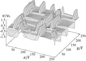
Figure 1: Normalized order parameter $\psi/\psi_{0}$ in a stripe intermediate state for $(\tau/\tau_{0},\alpha/\alpha_{0},v/v_{0})=(0.6,1.4,1)$. In the domains $\psi=\psi_{\rm s}$, $-\psi_{\rm s}$, or $0$.

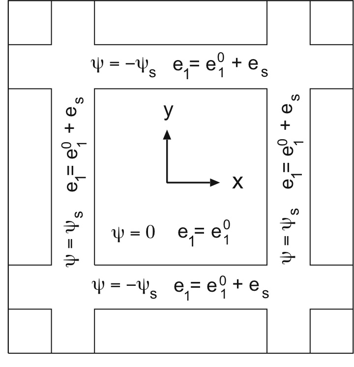
Figure 2: Disordered square regions are enclosed by ordered stripe domains uniaxially stetched along the $y$ or $x$ axis.

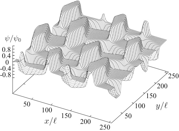
Figure 3: Normalized order parameter $\psi/\psi_{0}$ in a lozenge intermediate state for $(\tau/\tau_{0},\alpha/\alpha_{0},v/v_{0})=(0.6,1,1)$. In the domains $\psi=\psi_{\ell}$, $-\psi_{\ell}$, or $0$.

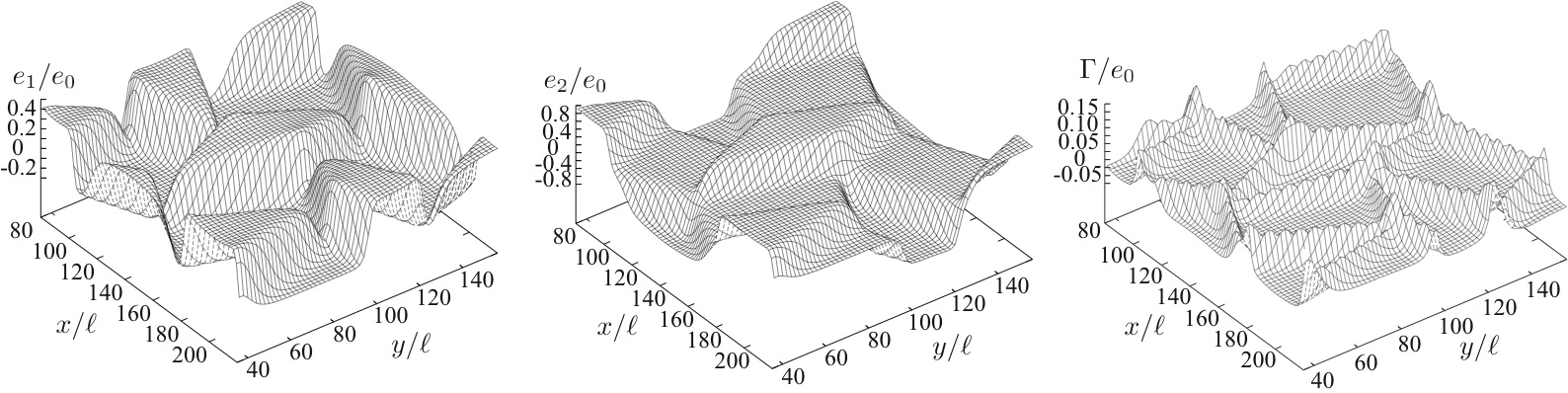
Figure 4: Strains $e_{1}$, $e_{2}$, and $\Gamma=e_{1}-\alpha\varphi/K$ in units of $e_{0}$ in Eq.(2.28) in the same lozenge state as in Fig. 3. These stains are flat and $\Gamma$ is small within the domains. As a result, $e_{1}=\alpha\varphi/K$, $e_{2}=g\psi/\mu$ in accord with Eq.(3.35).

III Phase transitions at fixed volume and shape

The phase transitions in solids can crucially depend on the boundary condition Onukibook ; comp . In this paper, we limit ourselves to the simplest case of fixed volume (area in 2D) and shape. This condition holds in the lateral directions if a solid film is fixed to a substrate. For 3D solids, the phase transition is usually observed under the stress-free boundary condition and claming of the boundaries is needed to realize the fixed-volume condition.

In this paper, we thus assume $A_{ij}=0$ ($i,j=x,y$) and

$$\langle{e_{1}}\rangle=\langle{e_{2}}\rangle=\langle{e_{3}}\rangle=0,$$ (3.1)

Furthermore, in our 2D simulation, there was no macroscopic order or

$$\langle{\psi}\rangle=0.$$ (3.2)

Then $\langle{\sigma_{xx}}\rangle=\langle{\sigma_{yy}}\rangle=-\alpha\langle{\psi^{2}}\rangle$ and $\langle{\sigma_{xy}}\rangle=0$. Note that $\langle{\psi}\rangle$ becomes nonvanishing under applied tetragonal strain $\langle{e_{2}}\rangle\neq 0$, since $\langle{e_{2}}\rangle$ plays a role of the ordering field in Eq.(2.27). In phase ordering, the condition (3.2) means that domains with positive $\psi$ and those with negative $\psi$ equally appear and the space average of $\psi$ over many domains vanishes. Under Eqs.(3.1) and (3.2) the elastic contribution $F_{\rm e}$ in Eq.(2.17) becomes

$$F_{\rm e}=\int d{\mbox{\boldmath$r$}}\bigg{[}-\frac{g^{2}}{2\mu}\psi^{2}+\frac{g^{2}K}{2\mu L}\chi^{2}-\frac{\alpha g}{L}\chi\varphi-\frac{\alpha^{2}}{2L}\varphi^{2}\bigg{]},$$ (3.3)

where $\varphi$ and $\chi$ are defined by Eqs. (2.19) and (2.25), respectively.

In our previous paper comp , the model with $\alpha>0$ and $g=0$ has been studied at fixed volume. There, in a temperature window, the free energy is lower in two-phase states than in one-phase states, where the domains attain macroscopic sizes, however. For $\alpha=0$ and $g>0$, on the other hand, lamellar or twin ordered states appear at low temperatures, where the interface normals make angles of $\pm\pi/4$ wth respect to the $x$ axis and $\chi$ vanishes in 2D Barsch ; pre ; Jacobs ; Curnoe ; Lookman ; Seme.

III.1 Stripe intermediate states

Figure 1 is an example of intermediate states consisting of ordered stripes parallel to the $x$ or $y$ axis. As illustrated in Fig. 2, the stripes enclose disordered rectangular regions with $\psi=0$ isotropically dilated at $e_{1}=e_{1}^{0}$. A rotation of $\pi/2$ of a stripe pattern yields another possible stripe pattern. As a result, the areal fractions of the stripes along the $x$ axis and those along the $y$ axis are the same under no applied tetragonal strain. We assume that the width of the stripes is much longer than the interface thickness. Within the stripes along the $y$ axis, we have

$$\psi=\psi_{\rm s},\quad e_{1}=e_{1}^{0}+e_{\rm s},\quad e_{2}=e_{\rm s}.$$ (3.4)

On the other hand, within the stripes along the $x$ axis, $\psi$ and $e_{2}$ are reversed in sign, but $e_{1}$ is unchanged, so that

$$\psi=-\psi_{\rm s},\quad e_{1}=e_{1}^{0}+e_{\rm s},\quad e_{2}=-e_{\rm s}.$$ (3.5)

Thus we have $\langle{\psi}\rangle=0$ and $\langle{e_{2}}\rangle=\langle{e_{3}}\rangle=0$ on the average. From the dilation-free condition $\langle{e_{1}}\rangle=e_{1}^{0}+\phi e_{s}=0$ in Eq.(3.1), the areal fraction of the ordered regions $\phi$ is expressed as

$$\phi=-e_{1}^{0}/e_{s}.$$ (3.6)

To calculate the excess dilation $e_{\rm s}$, we consider the interface region of a stripe along the $y$ axis, where all the quantities depend only on $x$. The mechanical equilibrium condition yields $\sigma_{xx}=$constant along the $x$ axis. Here $\nabla_{x}u_{x}$ changes along the $x$ axis, while $\nabla_{y}u_{y}$ remains at $e_{1}^{0}/2$. From Eq.(2.8) or from Eq.(2.26) $\nabla_{x}u_{x}$ across the interface is expressed as

$$\nabla_{x}u_{x}-\frac{1}{2}e_{1}^{0}=\frac{\alpha}{L}\psi(x)^{2}+\frac{g}{L}\psi(x),$$ (3.7)

where $L$ is defined in Eq.(2.23). The above quantity is equal to $e_{1}(x)-e_{1}^{0}$ and $e_{2}(x)$. The result (3.7) also follows from Eqs.(2.20) and (2.21), where $\cos 2\theta=1$ and $\chi=\psi$ since $\psi$ change along the $x$ axis. The order parameter $\psi(x)$ changes from 0 to $\psi_{s}$ with increasing $x$, leading to

$$e_{\rm s}=(\alpha\psi_{\rm s}^{2}+g\psi_{\rm s})/L,$$ (3.8)

In the extremum condition (2.14) for $\psi(x)$, we set $e_{1}-e_{1}^{0}$ and $e_{2}$ equal to the right hand side of Eq.(3.7) to obtain

$$C\frac{d^{2}\psi}{dx^{2}}=f_{0}^{\prime}-2\alpha e_{1}^{0}\psi-(g+2\alpha\psi)(\alpha\psi^{2}+g\psi)/L,$$ (3.9)

where $f_{0}^{\prime}=\partial f_{0}/\partial\psi$. This equation is integrated to give the standard form of the interface equation Onukibook ,

$$\frac{C}{2}\bigg{(}\frac{d\psi}{dx}\bigg{)}^{2}=f_{\rm st}(\psi),$$ (3.10)

where $f_{\rm st}(\psi)$ is the effective free energy density near the interface. Here the derivative $\partial f_{\rm st}(\psi)/\partial\psi$ is equal to the right hand side of Eq.(3.9) and $f_{\rm st}(0)=0$ is required, so we obtain

$$f_{\rm st} = f_{0}-\alpha e_{1}^{0}\psi^{2}-(g+\alpha\psi)^{2}\psi^{2}/2L$$ (3.11)

$$= \psi^{2}\bigg{[}\frac{\tau^{\prime}}{2}+\frac{{u}}{4}\psi^{2}+\frac{v}{6}\psi^{4}-\frac{\alpha}{L}g\psi\bigg{]},$$

In the second line, we define the coefficients,

$$\tau^{\prime} = \tau-g^{2}/L-2\alpha e_{1}^{0},$$ (3.12)

$$\beta_{L} = 2\alpha^{2}/L,$$ (3.13)

$$u = {\bar{u}}-2\alpha^{2}/L={\bar{u}}-\beta_{L}.$$ (3.14)

The integrand of $F_{\rm e}$ in Eq.(2.27) yields the above $f_{\rm st}$ if we replace $\langle{e_{1}}\rangle$ by $e_{1}^{0}$, $\delta\psi$ by $\psi$, $\chi$ by $\psi$, and $\varphi$ by $\psi^{2}$, with $\langle{e_{2}}\rangle=0$.

For the existence of a planar interface $f_{\rm st}(\psi)$ should be minimized at the two points $\psi=0$ and $\psi_{\rm s}$, so we need to require $f_{\rm st}=\partial f_{\rm st}/\partial\psi=0$ at $\psi=\psi_{\rm s}$. Hence $\psi_{\rm s}$ is the solution of the following cubic equation,

$$\bigg{(}\frac{\partial}{\partial\psi}\frac{f_{\rm st}}{\psi^{2}}\bigg{)}_{\psi=\psi_{\rm s}}=\frac{{u}}{2}\psi_{\rm s}+\frac{2v}{3}\psi_{\rm s}^{3}-\frac{\alpha}{L}g=0.$$ (3.15)

where $\tau$ vanishes and $\psi_{\rm s}$ turns out to be independent of $\tau$ or the temperature. In Appendix A, we will explicitly solve the above cubic equation. From $f_{\rm st}(\psi_{\rm s})=0$ the effective reduced temperature $\tau^{\prime}$ is related to $\psi_{\rm s}$ by

$$\tau^{\prime} = \frac{2\alpha}{L}g\psi_{\rm s}-\frac{{u}}{2}\psi_{\rm s}^{2}-\frac{v}{3}\psi_{\rm s}^{4},$$ (3.16)

$$= \frac{\alpha}{L}g\psi_{\rm s}+\frac{{v}}{3}\psi_{\rm s}^{4},$$

where the quadratic term in the first line is eliminated in the second line with the aid of Eq.(3.15). Thus $\tau^{\prime}$ is also a constant independent of $\tau$. With Eqs.(3.13) and (3.14), we may rewrite $f_{\rm st}$ as

$$f_{\rm st}=\psi^{2}(\psi-\psi_{\rm s})^{2}\bigg{[}\frac{v}{6}(\psi+\psi_{\rm s})^{2}+\frac{v}{3}\psi_{\rm s}^{2}+\frac{u}{4}\bigg{]}.$$ (3.17)

Since $f_{\rm st}(\psi)>0$ should hold at $\psi=-\psi_{\rm s}$, the inequality $v\psi_{\rm s}^{2}/3+u/4>0$ follows, which then gives $\psi_{\rm s}>0$ from Eq.(3.15). The positivity $\tau^{\prime}>0$ also holds.

From Eq. (3.12) we have $e_{1}^{0}=(\tau-g^{2}/L-\tau^{\prime})/2\alpha$. Use of Eqs. (3.8) and (3.16) gives the areal fraction $\phi$ in Eq.(3.6) in the form,

$$\phi=(\tau_{\rm s}-\tau)/\tau_{\rm sw}.$$ (3.18)

Here $\tau_{\rm s}=\tau^{\prime}+g^{2}/L$ and $\tau_{\rm sw}={2\alpha}e_{\rm s}$ are rewritten as

$$\tau_{\rm s}=\frac{g^{2}}{L}+\frac{\alpha}{L}g\psi_{\rm s}+\frac{{v}}{3}\psi_{\rm s}^{4},$$ (3.19)

$$\tau_{\rm sw}=\frac{2}{L}\alpha\psi_{\rm s}(g+\alpha\psi_{\rm s}).$$ (3.20)

Since $\phi\rightarrow 0$ as $\tau\rightarrow\tau_{\rm s}$, $\tau_{\rm s}$ is the transition-point value of $\tau$. From $0<\phi<1$, $\tau$ is in the window range,

$$\tau_{\rm s}-\tau_{\rm sw}<\tau<\tau_{\rm s},$$ (3.21)

to realize the stripe domain morphology. For $\tau<\kern-12.0pt\lower 5.0pt\hbox{$\displaystyle=$}\tau_{\rm s}-\tau_{\rm sw}$ the system changes into an ordered state (where the order parameter and the free energy will be calculated as Eqs.(3.47) and (3.48), respectively).

In the stripe intermediate states, the free energy density in the disordered regions is $f_{\rm el}=K(e_{1}^{0})^{2}/2$, while that in the stripes is $f_{0}+f_{\rm el}+f_{\rm int}=Ke_{1}^{0}(e_{1}^{0}/2+e_{\rm s})$ from $f_{\rm st}(\psi_{\rm s})=0$ or from Eq.(3.16), where $e_{\rm s}$ is the excess dilation given in Eq.(3.8). Neglecting the surface contribution, we write the free energy density as

$$\frac{F}{V} = \frac{K}{2}e_{1}^{0}(e_{1}^{0}+2\phi e_{\rm s})$$ (3.22)

$$= -\frac{K}{8\alpha^{2}}(\tau_{\rm s}-\tau)^{2},$$

where the first line holds for general $e_{1}^{0}$ and the second line follows from Eq.(3.6) at fixed volume. Thus $F$ is negative in the stripe intermediate phase.

III.2 Lozenge intermediate states

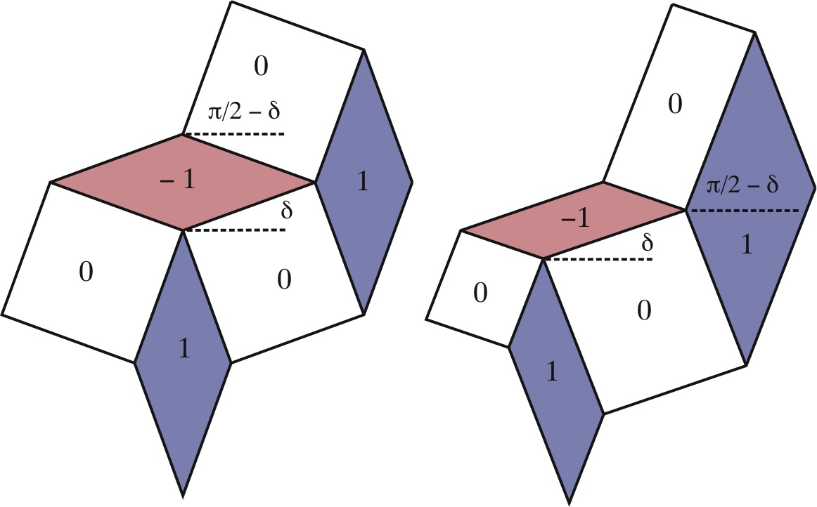
Figure 5: Illustration of the lozenge geometry. Symmetric pattern consisting of lozenges and squares (left) and asymmetric pattern consisting of parallelograms and rectangles (right). The angles of the interface normals with respect to the horizontal axis are written in terms of the angle $\delta$. The numbers $1$, $-1$, and 0 denote the value of $\psi(x,y)/\psi_{\ell}$.

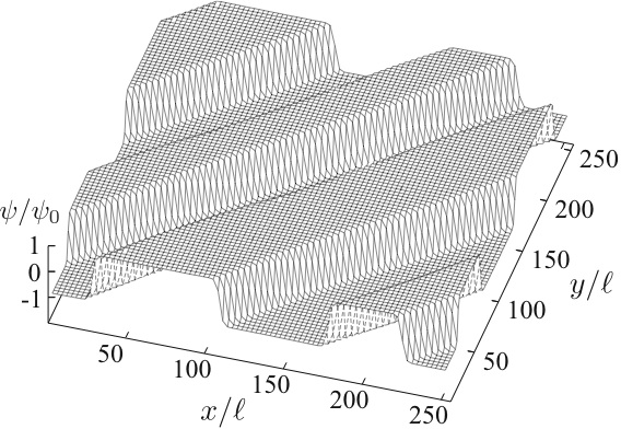
Figure 6: Normalized order parameter $\psi/\psi_{0}$ in a twin state consisting of two ordered variants separated by interfaces for $(\tau/\tau_{0},\alpha/\alpha_{0},v/v_{0},)=(-1,1,1)$, where $\psi_{0}$, $\tau_{0}$, $\alpha_{0}$, and $v_{0}$ are given in Eqs.(2.28) and (2.30) and the spatial scale is $\ell$ in Eq.(2.29).

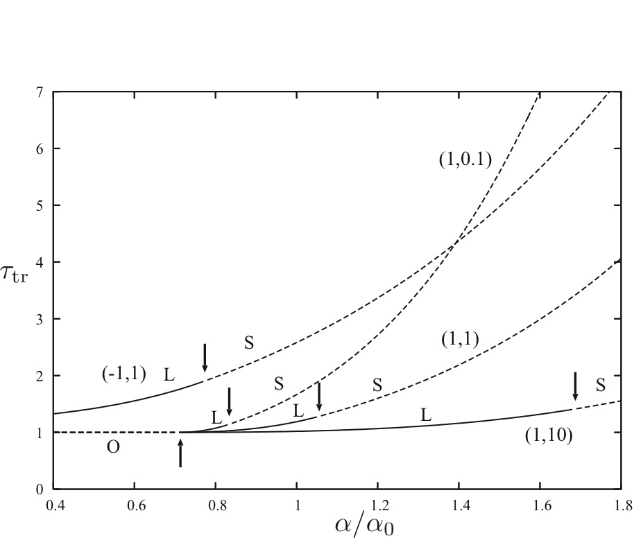
Figure 7: Reduced transition temperature $\tau_{\rm tr}$ (maximum of $\tau_{\rm s}$, $\tau_{\ell}$, and $\tau_{0c}$) in units of $\tau_{0}$ as functions of $\alpha/\alpha_{0}$. The numbers to each curve represent $(\bar{u}/|\bar{u}|,v/v_{0})$. The transition is from disordered to lozenge states on the solid lines (L). At the upward arrow $\delta\rightarrow\pi/4$, and on its left (O) the transition is to twin ordered states. At the downward arrows $\delta\rightarrow 0$, and on their right (S) the transition is to stripe states.

We show another kind of intermediate states. In Fig, 3, the pattern consists of ordered lozenges (rhombus) with $\psi=\pm\psi_{\ell}$ and disordered squares with $\psi=0$. As in Fig. 4, the strains $e_{1}$ and $e_{2}$ change mostly in the interface regions and are nearly flat (homogeneous) within each domain. The geometry is illustrated in Fig. 5. The ordered domains are characterized by the lozenge angle $\delta$ in the range $0<\delta<\pi/4$. More generally, as shown on the right, the pattern may consist of ordered parallelograms (quadrilaterals with both pairs of opposite sides being parallel) and disordered rectangles. The stepwise behavior of the strains in each domain in Fig. 4 is a characteristic feature of the lozenge geometry in Fig.5. We may derive it starting with the assumption of the stepwise behavior of $\psi$. We first examine the behavior of $\chi$ in Eq.(2.25) in the vicinity of an interface between ordered and disordered domains. Except near the corners of the lozenges, we may set

$$\psi(x,y)=\pm\psi_{\ell}\Psi(\zeta),$$ (3.23)

where $+$ (or $-$) is for the ordered phase with $\psi=\psi_{\ell}$ (or $\psi=-\psi_{\ell}$) and $\zeta$ is the coordinate along the interface normal direction ${\mbox{\boldmath$n$}}=(n_{x},n_{y})$. The function $\Psi(\zeta)$ tends to unity in the interior of all the ordered domains, while it vanishes in the disordered regions. From Eq.(2.25) we obtain ${d^{2}\chi}/{d\zeta^{2}}=\pm\cos(2\theta_{0})\psi_{\ell}{d^{2}\Psi}/{d\zeta^{2}}$, where $\cos(2\theta_{0})=n_{x}^{2}-n_{y}^{2}$ with $\theta_{0}$ being the angle between $n$ and the $x$ axis. From Fig. 5 we can see that $\theta_{0}=\pm\delta$ (or $\theta_{0}=\pi/2\pm\delta$) for the ordered phase with $\psi=\psi_{\ell}$ (or for that with $\psi=-\psi_{\ell}$) so that $\cos(2\theta_{0})=\pm\cos(2\delta)$. Thus we find

$$\frac{d^{2}\chi}{d\zeta^{2}}=\cos(2\delta)\psi_{\ell}\frac{d^{2}\Psi}{d\zeta^{2}},$$ (3.24)

where the symbol $\pm$ has disappeared. This is satisfied if $\chi-\cos(2\delta)\psi_{\ell}\Psi$ is a constant or if

$$\chi(x,y)=[\Psi(x,y)-\phi]\psi_{\ell}\cos(2\delta),$$ (3.25)

where $\phi=\langle{\Psi}\rangle$ is the areal fraction of the ordered regions and $\langle{\chi}\rangle=0$ is satisfied (since $\Psi(x,y)$ is equal to 1 in the ordered regions and to 0 in the disordered regions). We numerically calculated $\chi(x,y)$ from the inverse Fourier transformation of $\chi_{\mbox{\boldmath$k$}}=(k_{x}^{2}-k_{y}^{2})\psi_{\mbox{\boldmath$k$}}/k^{2}$ to confirm the above relation for a number of the lozenge states, where the agreement becomes better with decreasing the interface width (or decreasing the coefficient $C$ in Eq.(2.1)). Similarly, the strain $e_{2}(x,y)$ is proportional to $\psi(x,y)$ and is of the form,

$$e_{2}(x,y)=[g-K\Gamma_{c}\cos(2\delta)]\psi(x,y)/\mu.$$ (3.26)

where we define

$$\Gamma_{c}=[g\cos(2\delta)-\alpha\mu\psi_{\ell}/K]\psi_{\ell}/L.$$ (3.27)

Here the inverse Fourier transformation of $\alpha\varphi_{\mbox{\boldmath$k$}}\cos(2\theta)$ in Eq.(2.,21) has been approximated by $\alpha\cos(2\delta)\psi_{\ell}\psi(x,y)$. In the thin interface limit, $\psi(x,y)/\psi_{\ell}(=0,\pm 1)$ and $\Psi(x,y)(=0,1)$ are step functions and Eqs.(3.25) and (3.26) hold exactly as solutions of Eqs.(2.21) and (2.25).

We rewrite the elastic free energy in Eq.(3.3) as

$$F_{\rm e}=\int d{\mbox{\boldmath$r$}}\bigg{[}-\frac{g^{2}}{2\mu}\psi^{2}-\frac{\beta_{K}}{4}\varphi^{2}+\frac{KL}{2\mu}{\Gamma^{2}}\bigg{]}.$$ (3.28)

where we define the coefficient $\beta_{K}$ and introduce the quantity $\Gamma$ by

$$\beta_{K} = 2\alpha^{2}/K,$$ (3.29)

$$\Gamma = \frac{g}{L}\chi-\frac{\alpha\mu}{KL}\varphi.$$ (3.30)

Then $e_{1}=\Gamma+\alpha\varphi/K$ in terms of $\Gamma$. From Eq.(3.24) we find $\Gamma=(1-\phi)\Gamma_{c}$ in the ordered regions and $\Gamma=-\phi\Gamma_{c}$ in the disordered regions with $\Gamma_{c}$ being defined by Eq.(3.27), so that $\langle{\Gamma}\rangle=0$ and $\langle{\Gamma^{2}}\rangle=\phi(1-\phi)\Gamma_{c}^{2}$. In addition $\langle{\varphi^{2}}\rangle=\psi_{\ell}^{4}\phi(1-\phi)$. Neglecting the surface tension contribution, we may calculate the average free energy density as

$$\frac{F}{V}=f(\psi_{\ell})\phi+\bigg{[}-\frac{\beta_{K}}{4}\psi_{\ell}^{4}+\frac{KL}{2\mu}{\Gamma_{c}^{2}}\bigg{]}\phi(1-\phi).$$ (3.31)

For simplicity, we introduce

$$f(\psi)=f_{0}(\psi)-{g^{2}}\psi^{2}/2\mu,$$ (3.32)

which is of the same form as $f_{0}$ in Eq.(2.2) with $\tau$ being shifted to $\tau-g^{2}/\mu$.

The average free energy in Eq.(3.31) depends on $\delta$, $\psi_{\ell}$, and $\phi$. In our simulation to follow, we shall see that both the symmetric and asymmetric patterns in Fig. 5 both appear and the edges of the ordered regions are flattened with decreasing $\tau$ (Figs. 11 and 14). This means that $\delta$ and $\phi$ can be varied independently, though they are related as $\phi=\sin(2\delta)/(1+\sin(2\delta))$ for the symmetric pattern (left of Fig.5). Thus we minimize $F$ with respect to these three quantities. First, from Eq.(3.27) we notice that ${\Gamma_{c}}$ can vanish for

$$\alpha\mu\psi_{\ell}/gK<1,$$ (3.33)

if the angle $\delta$ is chosen as

$$\delta=\frac{1}{2}\cos^{-1}(\alpha\mu\psi_{\ell}/gK).$$ (3.34)

If we set $\Gamma=0$ or $\chi=(\alpha\mu/gK)\varphi$, we obtain

$$e_{1}=\alpha\varphi/K,\quad e_{2}=g\psi/\mu,$$ (3.35)

where the former follows from Eq.(2.26) and the latter from Eq.(2.21) or from Eq.(3.36). The snapshots in Fig. 4 are consistent with the above relations except in the interface regions.

Under Eqs.(3.34) and (3.35) we furthermore minimize $F/V$ with respect to $\psi_{\ell}$ and $\phi$. If $\Gamma_{c}=0$, the coefficient of the quadratic term $(\propto\phi^{2})$ is positive in Eq.(3.31) and $F/V$ can take a minimum as a function of $\phi$ in the range $0<\phi<1$ for sufficiently small $f(\psi_{\ell})$. From Eq.(3.31) the minimum conditions read

$$\frac{1}{\phi V}\frac{\partial F}{\partial\psi_{\ell}}=f^{\prime}(\psi_{\ell})-\beta_{K}\psi_{\ell}^{3}(1-\phi)=0,$$ (3.36)

$$\frac{1}{V}\frac{\partial F}{\partial\phi}=f(\psi_{\ell})-\frac{1}{4}\beta_{K}\psi_{\ell}^{4}(1-2\phi)=0,$$ (3.37)

where $f^{\prime}=\partial f/\partial\psi$. The first equation (3.36) is equivalent to the equilibrium condition (2.14) outside the interface regions if use is made of Eq.(3.35). In our previous work on the compressible Ising modelcomp , similar mminimization of $F$ yielded two-phase coexistence in a temperature window (leading to Eqs.(3.49)-(3.52) in the next subsection). In the present case, we may eliminate $\phi$ from Eqs.(3.36) and (3.37) to obtain $\psi f^{\prime}-2f-\beta_{K}\psi^{4}/2=0$ at $\psi=\psi_{\ell}$. This is solved to give

$$\psi_{\ell}^{2}={3}(\beta_{K}-\bar{u})/4v,$$ (3.38)

from which we need to require $\beta_{K}>\bar{u}$. Remarkably, $\psi_{\ell}$ becomes independent of $\tau$ as well as $\psi_{\rm s}$ determined by Eq.(3.15). From Eq.(3.36) the areal fraction $\phi$ is expressed as

$$\phi=1-f^{\prime}(\psi_{\ell})/\beta_{K}\psi_{\ell}^{3}=(\tau_{\ell}-\tau)/\tau_{\ell{\rm w}},$$ (3.39)

in the same form as in Eq.(3.18). Here,

$$\tau_{\ell}=\frac{g^{2}}{\mu}+\frac{v}{3}\psi_{\ell}^{4}=\frac{g^{2}}{\mu}+\frac{3}{16v}(\beta_{K}-\bar{u})^{2},$$ (3.40)

$$\tau_{\ell{\rm w}}=\beta_{K}\psi_{\ell}^{2}=\frac{3}{4v}\beta_{K}(\beta_{K}-\bar{u}).$$ (3.41)

The $\tau_{\ell}$ is the transition reduced temperature and $\tau_{\ell{\rm w}}$ is the width of the window. The lozenge intermediate phase is realized in the window,

$$\tau_{\ell}-\tau_{\ell{\rm w}}<\tau<\tau_{\ell}.$$ (3.42)

As in Eq.(3.22) the average free energy density is calculated as

$$\frac{F}{V}=-\frac{K}{8\alpha^{2}}(\tau_{\ell}-\tau)^{2}.$$ (3.43)

Now we return to Eq. (3.33) and the inequality $\beta_{K}>\bar{u}$ implied by Eq.(3.38). They impose the range of $\beta_{K}=2\alpha^{2}/K$ allowed for the lozenge phase,

$${\bar{u}}<\beta_{K}<\frac{\bar{u}}{2}+\sqrt{\frac{\bar{u}^{2}}{4}+\frac{8g^{2}}{3\mu^{2}}Kv}.$$ (3.44)

Here Eq.(3.33) gives the upper bound, at which $\delta$ tends to $0$ and the lozenge patterns continuously change into those of stripes. Therefore, the lozenge-stripe boundary is determined by $\psi_{\ell}=gK/\mu\alpha$, at which $\psi_{\rm s}=\psi_{\ell}$, leading to $\tau_{\rm s}=\tau_{\ell}$ from Eqs.(3.19) and (3.40). The continuity of $F/V$ also holds from Eqs.(3.22) and (3.43).

III.3 One-dimensionally ordered states

With decreasing $\tau$, our system eventually consists of regions of two ordered variants with $\psi=\pm\psi_{\rm e}$ at fixed volume and shape in steady states. In Fig. 6, we show such a lamellar or twin ordered state, where the two ordered variants are separated by antiphase boundaries or twin walls and there is no bulk disordered region Barsch ; pre ; Jacobs ; Curnoe ; Lookman . Here we assume that all the quantities depend only on $x^{\prime}=(x-y)/\sqrt{2}$ as in Fig.6. Then we obtain $\chi=0$, leading to $e_{1}=\alpha\varphi/L$, and $e_{2}=g\psi/\mu$. The resultant free energy at fixed volume is expressed as

$$F=\int d{\mbox{\boldmath$r$}}\bigg{[}f+\frac{C}{2}|{\psi^{\prime}}|^{2}-\frac{\beta_{L}}{4}\varphi^{2}\bigg{]},$$ (3.45)

where $\psi^{\prime}=d\psi/dx^{\prime}$ and $\beta_{L}$ is defined by Eq.(3.13). The above form coincides with the free energy of the compressible Ising model at fixed volume (with no ordering field conjugate to $\psi$) comp , on the basis of which we discuss the two cases below.

If $u={\bar{u}}-\beta_{L}$ in Eq.(3.14) is positive, a twin ordered state is realized for

$$\tau<\tau_{0c}=g^{2}/\mu,$$ (3.46)

where we may set $\varphi=0$ and then $\psi_{\rm e}$ is the solution of $f^{\prime}(\psi_{\rm e})=0$ with $f$ being defined by Eq.(3.32). It is solved to give

$$\psi_{\rm e}^{2}=[{\bar{u}}^{2}-4v(\tau-g^{2}/\mu)]^{1/2}/2v-{\bar{u}}/2v.$$ (3.47)

The elasticity effect is only to shift $\tau$ to $\tau-g^{2}/\mu$. The average free energy density takes a negative value,

$$F/V=-\psi_{\rm e}^{4}(3\bar{u}+4v\psi_{\rm e}^{2})/12,$$ (3.48)

where the surface tension contribution is neglected.

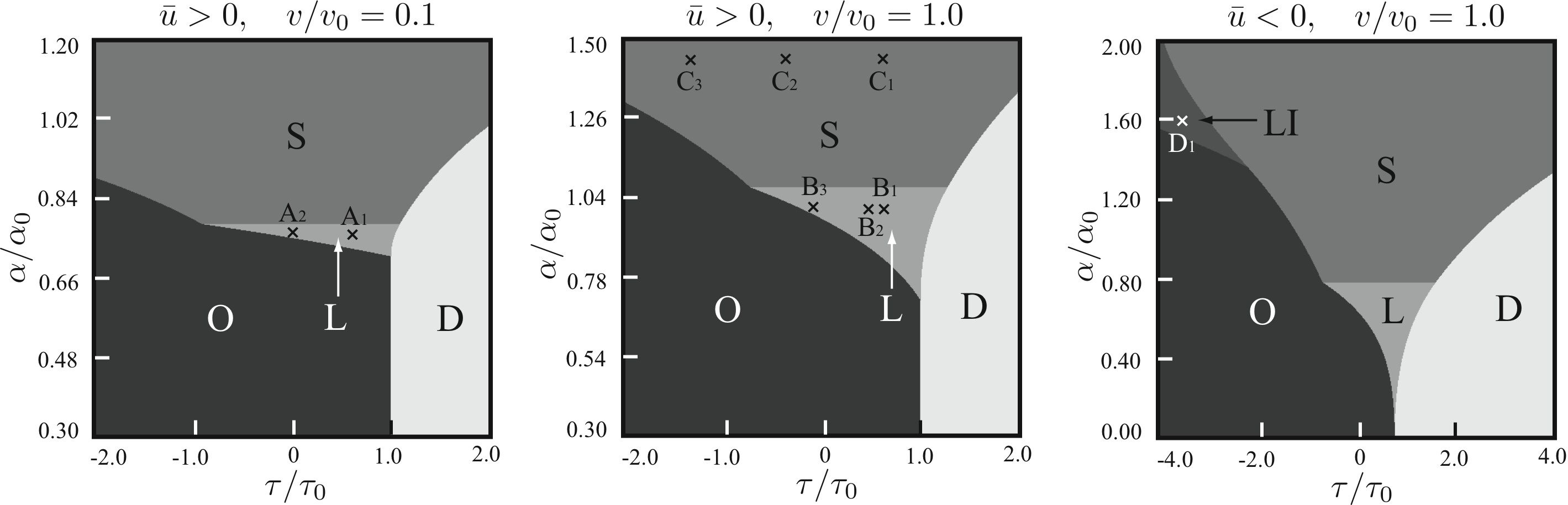
Figure 8: Theoretical phase diagrams in the plane of $\tau/\tau_{0}$ and $\alpha/\alpha_{0}$ for $({\bar{u}}/|{\bar{u}}|,v/v_{0})=(1,0.1)$ (left), $(1,1)$ (middle), and $(-1,1)$ (right). For ${\bar{u}}>0$, we have the disordered (D), twin ordered (O), stripe intermediate (S), and lozenge intermediate (L) phases. For ${\bar{u}}<0$ (right), there appears the lamellar intermediate phase (LI), where the disordered and ordered regions coexist macroscopically comp . The points A₁, B₁, B₂, C₁, C₂, and C₃ represent intermediate states with patterns shown in Figs. 9-13. At the points A₂ and B₃ twin patterns were realized numerically.

For $u={\bar{u}}-\beta_{L}<0$, on the other hand, the elastic term proportional to $\beta_{L}$ in Eq.(3.45) can give rise to macroscopic coexistence of disordered and ordered regions in the following window,

$$\tau_{0c}^{\prime}-\tau_{0w}<\tau<\tau_{0c}^{\prime},$$ (3.49)

where $\psi=\pm(3|u|/4v)^{1/2}$ in the ordered regions. The transition-point value and the window width in this case are given by

$$\tau_{0c}^{\prime} = \frac{g^{2}}{\mu}+\frac{3{u}^{2}}{16v}=\frac{g^{2}}{\mu}+\frac{3}{16v}(\beta_{L}-\bar{u})^{2},$$ (3.50)

$$\tau_{0w} = \frac{3\beta_{L}}{4v}|u|=\frac{3}{4v}\beta_{L}(\beta_{L}-\bar{u}).$$ (3.51)

The areal fraction of the ordered regions is $\phi=(\tau_{0c}^{\prime}-\tau)/\tau_{0w}$. The average free energy without the surface tension contribution becomes

$$\frac{F}{V}=-\frac{L}{8\alpha^{2}}(r_{0c}^{\prime}-r)^{2}.$$ (3.52)

Below the lower bound of the window in Eq.(3.49) the twin ordered phase with $\psi=\pm\psi_{\rm e}$ is realized. In our simulation, however, we did not realize the macroscopic coexistence predicted above.

III.4 Theoretical phase behavior

As $\tau$ is lowered from a value in a disordered state below a reduced transition temperature $\tau_{\rm tr}$, phase ordering occurs into an intermediate or ordered state. Depending on which is largest, $\tau_{\rm tr}$ is given by either of $\tau_{\rm s}$ in Eq.(3.19), $\tau_{\ell}$ in Eq.(3.40) under Eq.(3.44), $\tau_{0c}$ in Eq.(3.46) for $u>0$, or $\tau_{oc}^{\prime}$ in Eq.(3.50) for $u<0$. In Fig. 7, we show it as a function of $\alpha/\alpha_{0}$ for four sets of $({\bar{u}}/|{\bar{u}}|,v/v_{0})$ at $\mu=K$. (i) For $\bar{u}>0$, the transition is at $\tau=g^{2}/\mu$ to the twin phase for $\alpha/\alpha_{0}<\sqrt{2}$, to the lozenge phase for the intermediate range,

$$\sqrt{2}<\alpha/\alpha_{0}<\sqrt{1+A},$$ (3.53)

where $A\equiv(1+32K^{2}v/3\mu^{2}v_{0})^{1/2}$ from Eq.(3.44). For larger $\alpha/\alpha_{0}$ the stripe phase is realized. (ii) For ${\bar{u}}<0$, the transition is to the lozenge phase for $\alpha/\alpha_{0}<\sqrt{1+A}$ and to the stripe phase for $\alpha/\alpha_{0}>\sqrt{1+A}$.

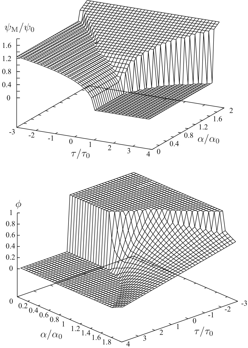
Figure 9: Theoretical order parameter $\psi_{M}$ scaled by $\psi_{0}$ (upper plate), which is $\psi_{\rm s}$, $\psi_{\ell}$, or $\psi_{\rm e}$ in the stripe, lozenge, or twin phase, respectively. Theoretical areal fraction $\phi$ of the ordered regions (lower panel) changing from 0 to 1 as $\tau$ is decreased. Here ${\bar{u}}>0$ and $v/v_{0}=1$ and the corresponding phase diagram is the middle plate of Fig. 8.

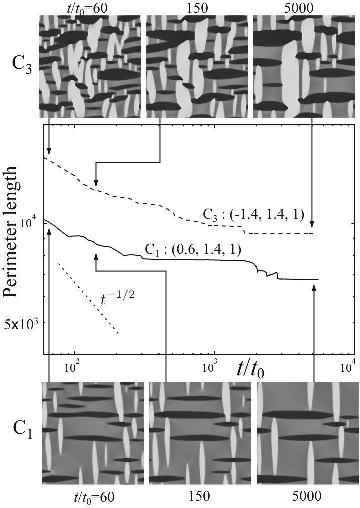
Figure 10: Relaxation of the total perimeter length after quenching from a disordered to stripe state at C₁ (lower curve) and C₃ (upper curve) in Fig. 8. Evolution of $\psi$ is displayed. Times are in units of $t_{0}$ in Eq.(4.1).

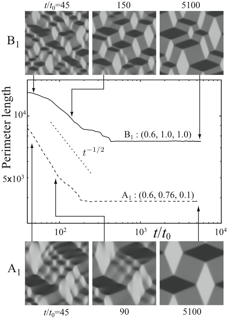
Figure 11: Relaxation from a disordered to lozenge state at A₁ (lower curve) and B₁ (upper curve) in Fig. 8. The final pattern is symmetric at A₁ and asymmetric at $B_{1}$ (see Fig. 5).

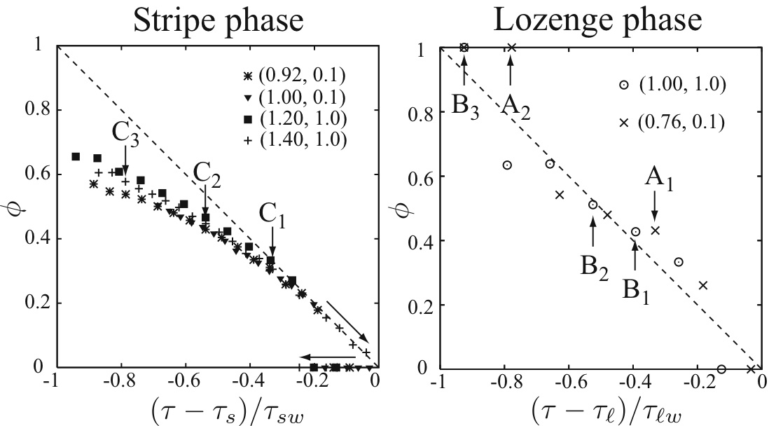
Figure 12: Numerical areal fraction of the ordered regions $\phi$ as a function of $(\tau-\tau_{\rm s})/\tau_{\rm sw}$ (left) and $(\tau-\tau_{\ell})/\tau_{\ell{\rm w}}$ (right) in the stripe and lozenge phases, respectively. The numbers are the values of $(\alpha/\alpha_{0},v/v_{0})$. See Fig. 8 for the positions of C₁, C₂, C₃, A₁, A₂, B₁, B₂, and B₃ in the phase diagrams. The arrows in the left panel indicate how the data were obtained in the range $g^{2}/\mu<\tau<\tau_{s}$.

We may calculate a phase diagram in the plane of $\tau/\tau_{0}$ and $\alpha/\alpha_{0}$ using the scalings in Eqs.(2.28)-(2.30) if we give $\mu/K$, $v/v_{0}$, and the sign of $\bar{u}$. Figure 8 displays such examples at $({\bar{u}}/|{\bar{u}}|,v/v_{0})=(1,0.1)$, $(1,1)$, and $(-1,1)$ at $\mu/K=1$. For ${\bar{u}}>0$, the plane is divided into the disordered (D), twin ordered (O), stripe (S), and lozenge (O) regions, depending on which morphology has the lowest free energy (the interface free energy being neglected). The lozenge region can appear for $\alpha/\alpha_{0}>\sqrt{2}$ from Eq.(3.44) and is narrow for small $v/v_{0}$ (or far from the tricriticality). The boundary between the lozenge and twin phases is determined by $\tau=\tau_{\ell}-\tau_{\ell w}$ (or $\phi=1$)). In fact, at this temperature, Eq.(3.47) gives $\psi_{\rm e}^{2}=3(\beta_{K}-\bar{u})/4v=\psi_{\ell}^{2}$ and $F/V$ in Eq.(3.48) becomes $-K\tau_{w}^{2}/8\alpha^{2}$, demonstrating the continuity of $\psi$ and $F/V$ at the boundary from Eqs.(3.38) and (3.52). For ${\bar{u}}<0$, the lamellar region is further divided into the ordered region (O) and the intermediate region of macroscopic two-phase coexistence (LI) described by Eqs.(3.49)-(3.52). The latter phase (LI) was not realized in our simulation, however.

Furthermore, in Fig. 9, we plot the equilibrium order parameter $\psi_{M}$ in the upper plate and the equilibrium areal fraction $\phi$ in the lower plate for ${\bar{u}}>0$ and $v/v_{0}=1$. The former is given by $\psi_{\rm s}$, $\psi_{\ell}$, or $\psi_{\rm e}$ in the stripe, lozenge, or twin phase, respectively. It is continuous at the disorder-twin and lozenge-twin boundaries and discontinuous at the other phase boundaries. The $\phi$ is between 0 and 1 in the intermediate phases. It is continuous at the disorder-stripe, disorder-lozenge, and lozenge-twin phase boundaries and discontinuous at the other phase boundaries. We can see that $\psi_{M}$ and $\phi$ are both discontinuous at the twin-stripe boundary.

IV Numerical results

We numerically integrated the dynamic equation (2.12) in 2D under the periodic boundary condition on a $256\times 256$ lattice. We measure space and time in units of $\ell$ in Eq.(2.29) and

$$t_{0}=\ell^{2}/\lambda_{0}C=K/\lambda_{0}g^{2},$$ (4.1)

where $\lambda_{0}$ is the kinetic coefficient. When we started with a disordered phase, the initial value of $\psi$ was a random number in the range $|\psi|<0.01\psi_{0}$ at each lattice point. No random source term was added to the dynamic equation. We calculated the strains $e_{1}$ and $e_{2}$ using their Fourier components in Eqs.(2.20) and (2.21) under the fixed volume condition. We set $\langle{e_{1}}\rangle=\langle{e_{2}}\rangle=0$. We will show the resultant patterns at the points marked by $\times$ in the phase diagrams in Fig. 8 (except A₂ and B₃). The parameters $(\tau/\tau_{0},\alpha/\alpha_{0},v/v_{0})$ are given by A₁$:(0.6,0.76,0.1)$, A₂$:(0,0.76,0.1)$, B₁$:(0.6,1,1)$, B₂$:(0.4,1,1)$, B₃$:(-0.2,1,1)$, C₁$:(0.6,1.4,1)$, C₂$:(-0.4,1.4,1)$, and C₃$:(-1.4,1.4,1)$.

IV.1 Transient behavior

In transient states, the ordered domains with positive (negative) $\psi$ tend to be elongated along the horizontal $x$ (vertical $y$) axis after their formation. They do not penetrate into the others belonging to the different variant (having the opposite $\psi$) on their encounters. Furthermore, thickening of the stripe shape is prohibited by the fixed-volume condition $\langle{e_{1}}\rangle=0$. As a result, our system tended to a nearly pinned state at long times in each simulation run.

In Fig. 10, we display the time evolution of the total perimeter length in the relaxation from disordered to stripe intermediate states at the points C₁ (where $\tau/\tau_{0}=0.6$) and C₃(where $\tau/\tau_{0}=-1.4$) in the middle panel of Fig. 8. The initial stage of domain formation is in the range $t/t_{0}<\kern-12.0pt\lower 5.0pt\hbox{$\displaystyle{\sim}$}10$ and the coarsening stops for $t/t_{0}>\kern-12.0pt\lower 5.0pt\hbox{$\displaystyle{\sim}$}10^{3}$. At the higher temperature (C₁), the ordered domains consist of long stripes with a smaller areal fraction. At the lower temperature (C₃), the domains are distorted, consisting of both large and small ordered stripes. In Fig. 11, we display the relaxation from disordered to lozenge intermediate states at the points A₁ and B₁ in the left and middle panels of Fig. 8. Here the domain pinning occurs at $t/t_{0}=2-4\times 10^{3}$. The patterns are nearly symmetric at A₁ but largely asymmetric at B₁. In these two cases, the lozenge angle $\delta$ and the areal fraction $\phi$ are nearly the same (see Fig. 12), while the domain sizes are considerably different.

IV.2 Steady intermediate states

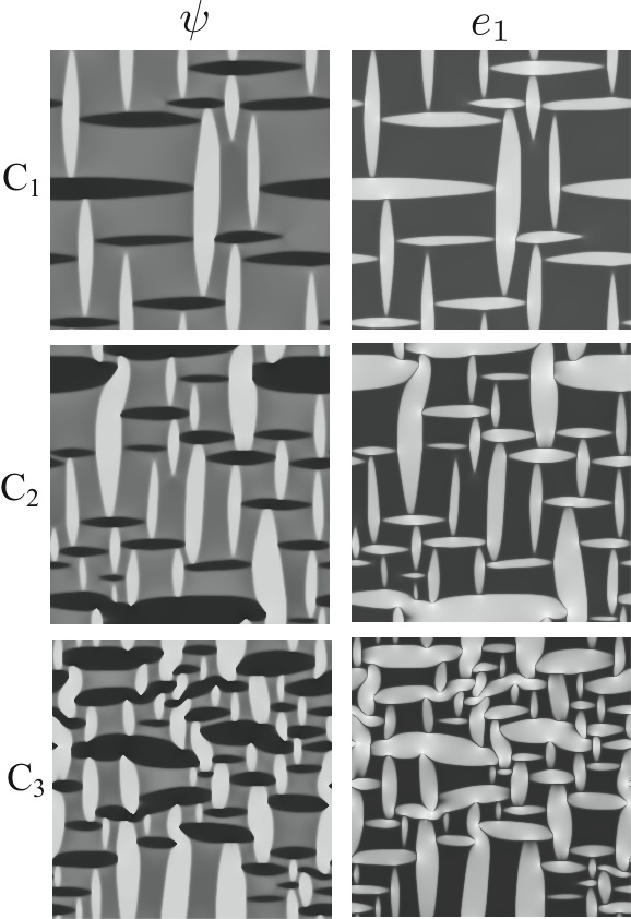
Figure 13: Stripe patterns of $\psi$ (left) and $e_{1}$ (right) at the points C₁, C₂, and C₃, where $\tau/\tau_{0}=0.6$, $-0.4$, and $-1.4$, respectively, with $\alpha/\alpha_{0}=1.4$ and $v/v_{0}=1$ being common. In the left panels, $\psi$ is positive in the white regions, negative in the black regions, and nearly zero in the gray regions. Our theory indicates $\psi=\psi_{\rm s},-\psi_{\rm s}$, or $0$ in the three regions. In the right panels, $e_{1}$ is positive in the white regions and negative in the black regions. Theoretically, $e_{1}=e_{1}^{0}+e_{\rm s}>0$ or $e_{1}=e_{1}^{0}<0$. See the corresponding $\phi$ in the left panel of Fig. 12.

Figure 14: Lozenge patterns of $\psi$ and $e_{1}$ at the points A₁ and B₂ in Fig. 8, where $(\tau/\tau_{0},\alpha/\alpha_{0},v/v_{0})=(0.6,0.76,0.1)$ and ($0.6,1,1)$, respectively. They are asymmetric ans symmetric, respectively, as in Fig. 5. At B₂ the edges are flattened, resulting in an increase of the ordered regions.

In our system, the disordered phase ($\psi=0$) is linearly stable for $\tau>g^{2}/\mu$ (as can be known from Eq.(3.3)). Therefore, we lowered $\tau$ below $g^{2}/\mu$ to produce ordered domains. Notice that the intermediate phase can be stable or have a negative free energy for $\tau$ above $g^{2}/\mu$ and below the transition-point value, as can be seen in Figs. 8 and 9. To realize such intermediate states, we increased $\tau$ starting with twin or intermediate states. Then $\phi$ decreased on approaching the transition point from below.

In Fig. 12, we show $\phi$ versus $(\tau-\tau_{\rm s})/\tau_{\rm sw}$ in the steady stripe states (left) and $\phi$ versus $(\tau-\tau_{\ell})/\tau_{\ell{\rm w}}$ in the steady lozenge states (right). Our theory predicts the linear dependence in Eqs.(3.18) and (3.39). The points A₁, A₂, B₁, B₂, B₃, C₁, C₂, and C₃ correspond to those in the phase diagrams in Fig. 8. Slightly below the transition, these numerical data excellently agree with our theory. In addition, in the left panel, we show the hysteresis behavior dependent on the initial condition in the range $g^{2}/\mu<\tau<\tau_{\rm s}$. But some discrepancies arise as $\tau$ approaches the lower bound of the temperature window. That is, as $\tau$ approach $\tau_{\rm s}-\tau_{\rm sw}$ in the left panel, $\phi$ become smaller than predicted and tend to saturate. In the right panel, twin states were realized at the points A₂ and B₃, though they are in the lozenge phase in our theory.

In Fig. 13, we show typical steady patterns of $\psi$ and $e_{1}$ in the stripe states C₁, C₂, and C₃ taken at $t/t_{0}=5\times 10^{3}$. The patterns of $e_{2}$ (not shown here) are almost indistinguishable from those of $\psi$. The patterns in Fig. 13 consist of long stripes for small $\phi$, but they contain even short ones and are considerably distorted for large $\phi$. Thus, as $\tau$ approaches $\tau_{\rm s}-\tau_{\rm sw}$, the domain morphology becomes more complex than in our theoretical picture. This explains why the data of $\phi$ in the left panel of Fig. 12 are below the theoretical straight line.

In Fig. 14, the lozenge pattern at the point A₁ is asymmetric with rectangular disordered regions, while that at the point B₂ is more symmetric and some disordered regions are nearly square. The $\phi$ for the pattern at B₂ is $0.51$ and is larger than those at A₁ and B₁ in Fig. 12 (being 0.42 and 0.43, respectively) by 20$\%$. The shapes of the lozenges at B₂ are more rounded than those at A₁ and B₁ with flattened edges. As a result, $\phi$ can be larger at B₂ than at B₁.

We stress that the intermediate patterns strongly depend on how they were created. They are sensitive even to the initial noise. For example, Figs. 11 and 14 show the lozenge patterns at the same point A₁ at $t/t_{0}=5\times 10^{3}$, where the large difference arises only from the initial noise. However, the pattern in Fig. 14 for A₁ will change into a more symmetric one at longer times. Note that the lozenge angle $\delta$ and the areal fraction $\phi$ are rather insensitive to the history. In fact, $\phi=0.41$ and $0.42$ for the point A₁ in Figs. 11 and 14, respectively.

V Summary and remarks

Though in 2D, we have presented a theory of intermediate states at structural phase transition using a minimal model with a one-component order parameter $\psi$ twofold coupled to the tetragonal strain properly $(g\neq 0)$ and to the dilational strain improperly ($\alpha\neq 0)$. The pinning of the domains is due to the nonlinearity (third and fourth order terms in the free energy) and there is no impurity. We summarize our main results.
(i) In Eq.(2.27) or in Eq.(3.3) we have derived the elastic free energy contribution $F_{\rm e}$ expressed in terms of $\psi$. It is very complicated due to the simultaneous presence of the proper coupling $(\propto g)$ and the improper coupling $(\propto\alpha)$.
(ii) For the stripe intermediate phase, the order parameter $\psi=\psi_{\rm s}$ within the ordered domains is determined by Eq.(3.15). The areal fraction $\phi$, the transition reduced temperature $\tau_{\rm s}$, and the width of the intermediate region $\tau_{\rm sw}$ are expressed as in Eqs.(3.18)-(3.20). The free energy decrease is of the simple form Eq.(3.22).
(iii) For the lozenge intermediate phase, the order parameter $\psi=\psi_{\ell}$ within the ordered domains is given by Eq.(3.38). The strains are approximately given by Eq.(3.35), where $\Gamma$ in Eq.(3.30) is small within the ordered domains. The areal fraction $\phi$, the transition reduced temperature $\tau_{\ell}$, and the width of the intermediate region $\tau_{\ell{\rm w}}$ are given in Eqs.(3.39)-(3.41). The free energy decrease is of the simple form Eq.(3.43).
(iv) We have compared the free energies in Eqs.(3.22), (3.43), (3.48), and (3.52) for the intermediate and ordered phases in the plane of $\tau$ and $\alpha$ with the other parameters held fixed. The transition reduced temperature, the phase diagrams, and the bird views of $\psi$ and $\phi$ are in Figs. 7-9, respectively. The intermediate states can appear in the case $\alpha>\kern-12.0pt\lower 5.0pt\hbox{$\displaystyle{\sim}$}\alpha_{0}$, where $\alpha_{0}$ is given in Eq.(2.30) and can be small near the tricritical point. Note that the ratio of the dilational strain and the tetragonal strains is of order $\mu/K$ for $\alpha\sim\alpha_{0}$.
(v) We have presented simulation results in 2D by integrating the dynamic equation (2.12). Figures 10 and 11 illustrate the freezing processes of the domain growth resulting in mesoscopic intermediate states. Figure 12 displays the areal fraction of the ordered regions obtained numerically. Figures 13 and 14 give typical patterns of the stripe and lozenge intermediate phases. These simulation results are consistent with our theory.

Further we give some remarks.
(1) In calculating the free energy $F$ in the intermediate states, we have neglected the surface tension contribution. This should be justified when the domain size much exceeds the surface thickness of order $\ell$ in Eq.(2.29).
(2) The previous 2D simulation in the strain-only theory Onukibook ; pre already produced the lozenge patterns in the presence of the third order term proportional to $e_{1}e_{2}^{2}$, which plays the same role as the dilational improper coupling in this paper.
(3) If a solid is compressed along one of the principal axes, the tetragonal extension along the compression axis becomes energetically unfavorable Onukibook ; JT , leading to a square-to-rectangle transition perpendicular to the axis. Then the transition could be described by a 2D theory with a one-component order parameter, although the lateral elastic deformations are much more complicated in real epitaxial films than treated in this paper Desai .
(4) In its present form, our theory cannot explain the 3D experiments Na ; Ohshima ; Shapiro ; Seto ; Kinoshita ; Uezu ; Waseda . We should construct a 3D theory of intermediate states. We will shortly report simulation results of intermediate states in 3D.

Appendix A Order parameter in stripe intermediate states

We here solve the cubic equation (3.15). For $u>0$ and $v=0$, we simply have $\psi_{\rm s}=2\alpha g/uL$. Including the case of $u<0$, we may generally solve it in the scaling form,

$$\psi_{\rm s}=\psi_{\rm t}\Phi(u/u_{\rm t}),$$ (A.1)

where we define two quantities,

$$\psi_{\rm t} = (3\alpha g/2Lv)^{1/3},$$ (A.2)

$$u_{\rm t} = 4v\psi_{\rm t}^{2}/3=(v/3)^{1/3}(4\alpha g/L)^{2/3}.$$ (A.3)

The scaling function $\Phi(w)$ is determined by

$$\Phi(w)^{3}+w\Phi(w)=1$$ (A.4)

with $\Phi(w)>0$ (since $\psi_{\rm s}>0$). This cubic equation can be solved to give an explicit expression for $\Phi(w)$. For $w>-3/4^{1/3}\cong-1.89$, it reads

$$\Phi=\bigg{(}\sqrt{\frac{w^{3}}{27}+\frac{1}{4}}+\frac{1}{2}\bigg{)}^{1/3}-\bigg{(}\sqrt{\frac{w^{3}}{27}+\frac{1}{4}}-\frac{1}{2}\bigg{)}^{1/3}.$$ (A.5)

For $w<-3/4^{1/3}$, it is expressed as

$$\Phi=2\bigg{|}\frac{w}{3}\bigg{|}^{1/2}\cos\bigg{[}\frac{1}{3}\cos^{-1}\bigg{(}\frac{1}{2}\bigg{|}\frac{3}{w}\bigg{|}^{3/2}\bigg{)}\bigg{]}.$$ (A.6)

We find $\Phi(w)\cong 1/w$ for $w\gg 1$ and $\Phi(w)\cong|w|^{1/2}$ for $w\ll-1$, so that

$$\psi_{\rm s} \cong 2\alpha g/uL\quad(u\gg u_{\rm t}),$$ (A.7)

$$\cong (3|u|/4v)^{1/2}\quad((u\ll-u_{\rm t}).$$

The first line holds for ${\bar{u}}\gg u_{\rm t}+\beta_{L}$, while the second line for $\beta_{L}\gg{\bar{u}}+u_{\rm t}$.

References

- (1) A. G. Khachaturyan, Theory of Structural Transformations in Solids, (John Wiley and Sons, New York, 1983).
- (2) A. Onuki, Phase Transition Dynamics (Cambridge University Press, Cambridge, 2002).
- (3) A. Nagasawa, J. Phys. Soc. Japan 40, 93 (1976).
- (4) M. Sugiyama, R. Ohshima, and F.E. Fujita, Trans. Jpn. Inst. Met., 27, 719 (1986).
- (5) S.M. Shapiro, Y. Noda, Y. Fujii, and Y. Yamada, Phys. Rev. B 30, 4314 (1984).
- (6) H. Seto, Y. Noda, and Y. Yamada, J. Phys. Soc. Japan 57, 3668 (1988); 59, 965 (1990); 59, 978 (1990).
- (7) Y. Fujii, S. Yoshioka, and S. Kinoshita, Ferroelectrics 303, 653 (2004).
- (8) H. Yokota, Y. Uesu, C. Malibert, and J-M. Kiat, Phys. Rev. B 75, 184113 (2007).
- (9) M. Nagao, T. Asaka, T. Nagai, D. Akahoshi, R. Hatakeyama, T. Yokosawa, M. Tanaka, H. Yoshikawa, A. Yamazaki, K. Kimoto, H. Kuwahara, and Y. Matsui, J. Phys. Soc. Jpn. 76 (2007) 103706.
- (10) S. Kartha, J. Krumhansl, J. Sethna and L. K. Wickham, Phys. Rev. B 52, 803 (1995).
- (11) A. Onuki, J. Phys. Soc. Japan 68, 5 (1999).
- (12) A. J. Mills, Nature 392, 147 (1998).
- (13) K.H. Ahn, T. Lookman, A.R. Bishop, Nature 428, 401 (2004); J. Appl. Phys. 99, 08A703 (2006).
- (14) A. Onuki, H. Nishimori, Phys. Rev. B 43 (1991) 13649. A. Onuki and A. Furukawa, Phys. Rev. Lett. 86 (2001) 452.
- (15) A. Onuki and S. Puri, Phys. Rev. E 59 (1999) R1331
- (16) E. S. Matsuo, M. Orkisz, S-T. Sun, Y. Li and T. Tanaka, Macromolecules, 27, 6791 (1994).
- (17) F. Ikkai and M. Shibayama, Phys. Rev. Lett. 82, 4946 (1999).
- (18) Y.H. Wen, Y. Wang, and L.Q. Chen, Phil. Mag. A. 80, 1967 (2000).
- (19) A. Onuki, J. Phys. Soc. Japan 70, 3479 (2001).
- (20) Zhi-Feng Huang and R. Desai, Phys. Rev. B 67 (2003) 075416.
- (21) G. R. Barsch and J. A. Krumhansl, Phys. Rev. Lett. 53, 1069 (1984).
- (22) A. E. Jacobs, Phys. Rev. B 46, 8080 (1992); ibid. 61, 6587 (2000).
- (23) A.E. Jacobs, S.H. Curnoe, and R.C. Desai, Phys. Rev. B 68, 224104 (2003).
- (24) R. Ahluwalia, T. Lookman, and A. Saxena, Acta Materialia, 54, 2109 (2006).
- (25) M. Artemev, Y. Wang and A.G. Khachaturyan, Acta Metall. 48, 2503 (2000).
- (26) R.B. Griffiths, Phys. Rev. B 7, 549 (1973).
- (27) A. Onuki and A. Minami, . Phys. Rev. B 76, 174427 (2007).