Code Diversity in Multiple Antenna Wireless Communication

Abstract

The standard approach to the design of individual space-time codes is based on optimizing diversity and coding gains. This geometric approach leads to remarkable examples, such as perfect space-time block codes [3], for which the complexity of Maximum Likelihood (ML) decoding is considerable. Code diversity is an alternative and complementary approach where a small number of feedback bits are used to select from a family of space-time codes. Different codes lead to different induced channels at the receiver, where Channel State Information (CSI) is used to instruct the transmitter how to choose the code. This method of feedback provides gains associated with beamforming while minimizing the number of feedback bits. Thus code diversity can be viewed as the integration of space-time coding with a fixed set of beams. It complements the standard approach to code design by taking advantage of different (possibly equivalent) realizations of a particular code design. Feedback can be combined with sub-optimal low complexity decoding of the component codes to match ML decoding performance of any individual code in the family. It can also be combined with ML decoding of the component codes to improve performance beyond ML decoding performance of any individual code. One method of implementing code diversity is the use of feedback to adapt the phase of a transmitted signal. Phase adaptation with the $4\times 4$ Quasi-Orthogonal Space-Time Block Code (QOSTBC) is shown to be almost information lossless; that is, this form of space-time coding does not reduce the capacity of the underlying multiple antenna wireless channel. Code diversity can also be used to improve performance of multi-user detection by reducing interference between users. Phase adaptation with two Alamouti users makes it possible for the Zero Forcing (ZF) or decorrelating detector to match the performance of ML joint detection. Code diversity implemented by selecting from equivalent variants is used to improve ML decoding performance of the Golden code. This paper introduces a family of full rate circulant codes which can be linearly decoded by fourier decomposition of circulant matrices within the code diversity framework. A $3\times 3$ circulant code is shown to outperform the Alamouti code at the same transmission rate.

I Introduction

Space-time codes improve the reliability of communication over fading channels by correlating signals across different transmit antennas. Two design criteria were proposed by Tarokh et al. [1]. The first is the rank criterion, which is to maximize the minimum rank ($r$) of the difference $X_{1}-X_{2}$ over all pairs of distinct codewords $X_{1},X_{2}$; the second is the determinant criterion, which is to maximize the minimum product ($\gamma$) of all nonzero singular values of the difference $X_{1}-X_{2}$ over all pairs of distinct codewords $X_{1},X_{2}$. The quantity $r$ is the diversity gain and the quantity $\gamma$ determines the coding gain. Diversity and coding gains determine the performance of space-time codes in the high $\mathop{\mathsf{SNR}}$ regime.

The ML decoder provides optimal decoding performance, but complexity typically becomes prohibitive as the constellation size increases. Sphere decoding [16] aims to reduce decoding complexity by restricting to a search over lattice points that lie in a sphere about an initial estimate. However when the channel matrix is close to singular (as will be the case on Line of Sight channels), the preprocessing stage of sphere decoding yields a plane of possibilities rather than a single initial estimate. Jaldén et al. [16] showed that overall expected complexity is exponential in transmission alphabet size and strongly dependent on signal to noise ratio ($\mathop{\mathsf{SNR}}$). Decoders such as the zero forcing decoder have low complexity but are suboptimal in terms of decoding performance.

Tan and Calderbank [9] introduced code diversity, a form of adaptive modulation where feedback is used to instruct the transmitter how to choose from a plurality of codes. In the case of QOSTBC, they showed that ML decoding of a particular code may be inferior (in terms of both error probability and decoding complexity) to a combination of adaptive modulation and suboptimal decoding. Bonnet et al. [19] examined the value of closed loop feedback in the context of the DSTTD and DABBA space-time block codes. Feedback is also examined by C. Lin et al. [18] in the context of beamforming.

This paper provides a general information theoretic framework for the analysis of code diversity. We show that it is possible to quantify and sometimes eliminate the gap between the error performance of low complexity zero forcing decoders and that of the optimal decoder. Code diversity increases the mutual information between the transmitted and received signals and it is possible to approach the information lossless property for certain codes, such as the QOSTBC [6, 7, 8, 9]. We introduce methods of inducing code diversity, such as adapting the phases of channel gains via a small number of feedback bits. Simulation shows that a small number of feedback bits are sufficient to obtain close to optimal decoding performance even with the simplest zero forcing decoder.

Feedback has also been used for opportunistic beamforming by Viswanath et al. [15] to optimize the total throughput for multi-user systems by modifying the phases of channel gains and the transmitted power at each transmit antenna. These authors show that opportunistic beamforming can approach the performance of perfect beamforming for systems with a large number of users. However it requires centralized processing and does not work as well for systems with fewer users. The focus of this paper is not sum capacity, rather it is improving the performance of individual links or joint detection of small number of users. Our use of phase adaptation avoids centralized processing and we demonstrate that our code diversity scheme brings significant improvement to the performance of general space-time codes and large reduction in decoding complexity.

We also introduce a family of full rate code designs based on circulant matrices within the code diversity framework. A universal linear decoder for this family of codes is also proposed based on fourier decomposition of circulant matrices. A $3\times 3$ circulant design is analyzed and shown to outperform the Alamouti code for a given transmission rate.

The paper is organized as follows. Section II presents the system model, Section III discusses fundamental limits on full rate space-time codes. Our code diversity scheme is introduced and analyzed in Section IV, applications are explored in Section V, and the new family of circulant codes is introduced in Section VI. Section VII provides conclusions.

II System Model

A space-time block codeword $X$ is represented as an $M\times T$ matrix, where the rows are indexed by transmit antennas and the columns are indexed by time slots. If $L$ distinct symbols are transmitted during one frame of $T$ symbol periods, then the transmission rate for the space time block code is $\frac{L}{T}$. In a system with $M$ transmit antennas and $N$ receive antennas, the received signal $\tilde{r}\in\mathcal{C}^{N\times T}$ is given by

$$\tilde{r}=\sqrt{\frac{E_{s}}{MN_{0}}}HX+\tilde{n}$$ (1)

where $H\in\mathcal{C}^{N\times M}$ is the channel matrix with entry $h_{ji}$ representing the channel gain between the $i^{th}$ transmit antenna and the $j^{th}$ receive antenna; $X\in\mathbb{C}^{M\times T}$ is a codeword with entries in the constellation $\mathbb{C}$; $\tilde{n}\in\mathcal{C}^{N\times T}$ is the normalized additive noise with entries as complex Gaussian with zero mean and unit variance, i.e.  $\mathcal{CN}(0,1)$; $N_{0}$ is the actual noise variance; and $E_{s}$ is average transmitted signal power.

An important feature of many algebraic constructions of space-time codes is transference of structure (correlation) at the transmitter to structure at the receiver. Transference means, we can rewrite (1) as:

$$r=\sqrt{\frac{E_{s}}{MN_{0}}}\mathcal{H}c+n$$ (2)

where $r\in\mathcal{C}^{NT\times 1};\;\ \mathcal{H}\in\mathcal{C}^{NT\times L}$; $c\in\mathbb{C}^{L\times 1}$ is the transmitted signal; and $n\in\mathcal{C}^{NT\times 1}$. Since $\mathop{\mathsf{SNR}}=\frac{E_{s}}{N_{0}}$, equation (2) can also be written as $r=\sqrt{\frac{\mathop{\mathsf{SNR}}}{M}}\mathcal{H}c+n$.

Equation (2) captures the perspective of the receiver, where the induced channel is assumed to be known, and the problem is to estimate the transmitted signals. Transference of structure from transmitter to receiver is possible for (real-valued) linear dispersion codes [5], the Golden code [12, 13, 14], the Silver code [26, 25, 27, 28, 29, 30] and many more.

We assume that the wireless channel is quasi-static, that is it remains constant over a frame and changes independently from one frame to the next.

II-A Channel Capacity

Given perfect CSI at the receiver, the channel capacity of the system with channel matrix $H$ is [4]:

$$C_{0}(M,N)=\mathbf{E}_{H}\log\det\left(I_{N}+\frac{E_{s}}{MN_{0}}HH^{{\dagger}}\right)$$ (3)

where, $\mathbf{E}_{H}$ is the expectation with respect to $H$.

For a specific space time block code with an induced channel matrix $\mathcal{H}$, the achievable maximum capacity is [11]:

$$C(M,N)=\frac{1}{T}\mathbf{E}_{\mathcal{H}}\log\det\left(I_{NT}+\frac{E_{s}}{MN_{0}}\mathcal{H}\mathcal{H}^{{\dagger}}\right)$$ (4)

The space time code is said to be information lossless if $C(M,N)=C_{0}(M,N)$.

For simplicity, we focuse on wireless systems with multiple transmit antennas and a single receive antenna (MISO).

III Fundamental Limits on Full Rate Codes

We consider full rate square designs $X$ that are linear and that employ QAM signaling. The average power constraint is expressed in terms of the Frobenius norm by $\|X\|_{F}^{2}\leq P$. Given linearity, the standard design criterion reduces to maximizing the minimum determinant among all possible codewords.

III-A Optimality of Orthogonal Designs

If $X$ is an $M\times M$ block space-time code with columns $C_{i}$, $i=1,\cdots,M$, then the hadamard inequality states

$$|\det{X}|\leq\prod_{i=1}^{M}||C_{i}||$$ (5)

Equality holds for orthogonal designs, that is when $C_{i}C_{j}^{{\dagger}}=0$ for all $i\neq j$.

G. Bresler and B. Hajek [20] proved that orthogonal designs also maximize the mutual information subject to an average power constraint on each symbol. For example, the Alamouti code is shown to be information lossless (namely maximizing mutual information with certain power constraints) for $2\times 1$ systems (see Hassibi and Hochwald [5]). It is easily seen that any $M\times M$ orthogonal design is information lossless for $M\times 1$ systems.

III-B Existence of Orthogonal Designs

Wolfe’s theorem [22] on amicable pairs of real orthogonal designs provides fundamental limits on the achievable rates of space-time block codes that employ complex signaling (see [21, 2, 23]). If $M=2^{h}M_{0}$, where $M_{0}$ is odd, then the maximum rate of a complex orthogonal design is $\frac{h+1}{M}$. When $M=2$, the Alamouti code is optimal, and when $M=4$, the orthogonal space-time code

$$X(x_{1},x_{2},x_{3})=\left(\begin{array}[]{cccc}x_{1}&x_{2}&x_{3}&0\\ -x^{*}_{2}&x^{*}_{1}&0&x_{3}\\ -x_{3}^{*}&0&x_{1}^{*}&-x_{2}\\ 0&-x^{*}_{3}&x_{2}^{*}&x_{1}\end{array}\right)$$ (6)

achieves the optimal rate.

Complex orthogonal designs maximize both the minimum determinant and mutual information, but fail to achieve full rate for more than two transmit antennas. Code diversity offers a way forward.

IV Code Diversity Through Phase Adaptation

The mechanism of phase adaptation is a simple and effective approach to code diversity. Other possible mechanisms are examined in section V.

IV-A Implementation

Equation (2) transfers structure at the transmitter (code structure) to structure at the receiver (induced channel structure). If there is no noise in (2), the ML estimate for the transmitted symbols $c$ is unique provided the column rank $\mathcal{R}(\mathcal{H})$ of channel matrix $\mathcal{H}$ is full, i.e.  $\mathcal{R}(\mathcal{H})=L$. This may not always be satisfied, and when $\mathcal{H}$ is close to rank deficient, decoding becomes unstable. We propose the following algorithm to combat rank deficiency of the channel matrix $\mathcal{H}$.

We allow the receiver to send back feedback to modify phases of channel gains as follows

$$h_{ij}\rightarrow h_{ij}\times e^{i\frac{2\pi k_{ij}}{K}}$$

where $k_{ij}\in\{1,2...,K\}$ is the feedback information, $K$ determines the number of feedback bits, and $\mathcal{H}^{{\dagger}}\mathcal{H}$ changes with different phase adaptations. Our algorithm only modifies phases of a small subset of the channel gains. For example, only the phase of one channel gain needs to be modified for systems with four transmit antennas and a single receive antenna.

Let $\{h_{ij}\}$ denote the set where the phases of channel gains $h_{ij}$ are modified and let $\{\hat{k}_{ij}\}$ denote the feedback selection information. Then the receiver selects $\{\hat{k}_{ij}\}$ which

• firstly maximizes $\mathcal{R}(\mathcal{H}^{{\dagger}}\mathcal{H})$ (Let $d_{\max}=\max\mathcal{R}(\mathcal{H}^{{\dagger}}\mathcal{H})$ )

• and secondly maximizes $\left(\prod_{i=1}^{d_{\max}}\omega_{i}\right)$, where $\omega_{i}$ are the nonzero eigenvalues of $\mathcal{H}^{\dagger}\mathcal{H}$.

If $d_{\max}=L$, i.e.  $\mathcal{H}^{{\dagger}}\mathcal{H}$ has full rank, then the receiver selects $\{\hat{k}_{ij}\}$ as

$$\{\hat{k}_{ij}\}=\mathop{\rm argmax}_{k_{ij}\in\{1,2...,K\}}det(\mathcal{H}^{{\dagger}}\mathcal{H})|_{\{h_{ij}\}\rightarrow\{h_{ij\times}e^{i\theta_{ij}}\}}$$ (7)

The structure in Fig. 1 illustrates our strategy for the system with two transmit antennas and one receive antenna, where feedback is used to adapt the phase of one channel gain.

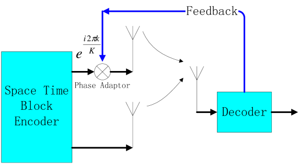
Figure 1: Code diversity implemented through phase adaptation for a system with two transmit antennas and one receive antenna.

Remark: In the above algorithm, code diversity is induced by different channel phase adaptations. Via feedback, the receiver can select the best code with a particular phase adaptation. Phase adaptation is also employed in [19]. Code diversity may also be induced in other ways.

In contrast with opportunistic beamforming, feedback is employed to increase reliability and achievable capacity and to enable low complexity decoders for each transmission. We now show that the above algorithm optimizes error performance for general space time codes and also maximizes achievable capacity $C(M,N)$ given in equation (4).

IV-B Analysis and Discussion

IV-B1 Analysis of Error Probability

For simplicity we restrict to systems with multiple transmit antennas and a single receive antenna ($N=1$). Assuming CSI at the receiver, the conditional probability of deciding $X^{\prime}$ when transmitting $X$ is:

$$P(X\rightarrow X^{\prime}|H)\leq exp(-\frac{E_{s}}{4MN_{0}}\parallel H(X-X^{\prime})\parallel_{F}^{2})$$ (8)

where, $\|\cdot\|_{F}$ denotes the matrix Frobenius norm (see [1]). Given (2), we rewrite (8) as

$$P(c\rightarrow c^{\prime}|\mathcal{H})\leq exp(-\frac{E_{s}}{4MN_{0}}\parallel\mathcal{H}(c-c^{\prime})\parallel_{F}^{2})$$ (9)

Then, the conditional average pairwise error probability is

$$\begin{array}[]{ll}P_{e|\mathcal{H}}=P(\hat{c}\neq c|\mathcal{H})\\ \leq\mathbf{E}_{D}\{exp(-\frac{E_{s}}{4MN_{0}}\parallel\mathcal{H}D\parallel_{F}^{2})\}\\ =\mathbf{E}_{D}\{exp(-\frac{E_{s}}{4MN_{0}}D^{\dagger}\mathcal{H}^{\dagger}\mathcal{H}D)\}\end{array}$$ (10)

where $D\triangleq c-c^{\prime}$.

To simplify this upper bound, we assume that $D\sim\mathcal{CN}(0,I_{L})$ and use the fact that

$$\mathbf{E}_{s}\{exp(-s^{\dagger}\Psi s)\}=\frac{exp(-\mu_{s}^{\dagger}\Psi[I+\Sigma\Psi]^{-1}\mu_{s})}{det(I+\Sigma\Psi)}$$ (11)

for $s\sim\mathcal{CN}(\mu_{s},\Sigma)$ and a Hermitian matrix $\Psi$.

We have

$$\begin{array}[]{ll}P_{e|\mathcal{H}}\leq\frac{1}{det(I_{L}+\frac{E_{s}}{4MN_{0}}\mathcal{H}^{\dagger}\mathcal{H})}=\frac{1}{\prod_{i=1}^{d}(1+\frac{E_{s}}{4MN_{0}}\omega_{i})}\\ \approx\left(\prod_{i=1}^{d}\omega_{i}\right)^{-1}\left(\frac{E_{s}}{4MN_{0}}\right)^{-d}.\end{array}$$ (12)

where $d=\mathcal{R}(\mathcal{H}^{\dagger}\mathcal{H})$ and $\omega_{i},i=1,\cdots,d$ are the nonzero eigenvalues of $\mathcal{H}^{\dagger}\mathcal{H}$. The diversity gain $d$ and coding gain $\left(\prod_{i=1}^{d}\omega_{i}\right)$ determine space-time code performance.

Code diversity optimizes space-time code performance by maximizing the diversity and coding gain.

Since $\mathcal{R}(\mathcal{H}^{\dagger}\mathcal{H})=\mathcal{R}(\mathcal{H})\leq\min(T,L)$, we have $d_{\max}=\min(T,L)$. For typical space-time block codes, $\min(T,L)\geq M$, and for such space-time block code, we have

$$P_{e|\mathcal{H}}\leq\left(\prod_{i=1}^{M}\omega_{i}\right)^{-1}\left(\frac{E_{s}}{4MN_{0}}\right)^{-M}$$ (13)

The above analysis shows that the error performance can be optimized by our code diversity scheme. Since $\mathcal{H}$ is adjusted to avoid rank deficiency, it is possible to employ low complexity zero-forcing decoding schemes.

IV-B2 Analysis of Achievable Capacity

The achievable capacity $C(M,N)$ in equation (4) can be further written as

$$\begin{array}[]{ll}C(M,N)=\frac{1}{T}\mathbf{E}_{\mathcal{H}}\log\prod_{i=1}^{d}\left(1+\frac{E_{s}}{MN_{0}}\omega_{i}\right)\\ \approx\frac{1}{T}\mathbf{E}_{\mathcal{H}}\log\left(\prod_{i=1}^{d}\omega_{i}\right)\left(\frac{E_{s}}{MN_{0}}\right)^{d}\end{array}$$ (14)

This shows that $\left(\prod_{i=1}^{d}\omega_{i}\right)$ and $d$ determine achievable capacity; the aim of code diversity is to maximize these quantities.

IV-B3 Discussion of Decoding Schemes

Given perfect CSI at the receiver, ML decoding achieves the optimal decoding performance at the receiver. For $2^{m}$-QAM signaling using the constellation $\mathbb{C}_{m}$, the ML decoding scheme is formulated as

$$\hat{c}=\mathop{\rm argmin}_{c\in\mathbb{C}_{m}^{L}}\|r-\sqrt{\frac{E_{s}}{MN_{0}}}\mathcal{H}c\|^{2}$$ (15)

Code diversity improves the performance/complexity tradeoff in decoding algorithms.

As the constellation size increases and the dimension of STBC goes up, ML decoding becomes computationally prohibitive. To reduce decoding complexity, we can adopt zero forcing decoding. However, near singularity of the channel matrix $\mathcal{H}$ in (2) reduces the effectiveness of these low-complexity schemes. Our proposed method increases the rank of the matrix $\mathcal{H}$ and avoids noise amplification. For the general receive structure (2), the simplest zero forcing decoding scheme is formulated as

$$\hat{c}=\mathop{\rm argmin}_{c\in\mathbb{C}_{m}^{L}}\|\mathcal{H}^{-1}r-\sqrt{\frac{E_{s}}{MN_{0}}}c\|^{2}$$ (16)

which decouples into $L$ subproblems each with linear decoding complexity. The value of code diversity is that the simplest zero forcing scheme is often good enough to obtain close to the performance of ML decoding of one of the constituent codes.

V Applications

V-A Quasi-Orthogonal Space Time Block Codes

In a system with four transmit antennas and one receive antenna, we consider the following quasi-orthogonal space time block code proposed by Jafarkhani [6]:

$$X=\left(\begin{array}[]{cccc}x_{1}&x_{2}&x_{3}&x_{4}\\ -x_{2}^{*}&x_{1}^{*}&-x_{4}^{*}&x_{3}^{*}\\ -x_{3}^{*}&-x_{4}^{*}&x_{1}^{*}&x_{2}^{*}\\ x_{4}&-x_{3}&-x_{2}&x_{1}\end{array}\right)$$ (17)

As shown in (13), the conditional average pairwise error probability for this QOSTBC under our code diversity scheme is upper bounded as

$$P_{e|\mathcal{H}}\leq\left(\prod_{i=1}^{4}\omega_{i}\right)^{-1}\left(\frac{E_{s}}{16N_{0}}\right)^{-4}$$ (18)

We now verify that our code diversity scheme optimizes the error performance and does not significantly reduce the capacity of the underlying multiple antenna wireless channel.

V-A1 Algorithm Implementation

With one receive antenna, the received signal can be written as

$$r=\left(\begin{array}[]{cccc}h_{1}&h_{2}&h_{3}&h_{4}\\ -h_{2}^{*}&h_{1}^{*}&-h_{4}^{*}&h_{3}^{*}\\ -h_{3}^{*}&-h_{4}^{*}&h_{1}^{*}&h_{2}^{*}\\ h_{4}&-h_{3}&-h_{2}&h_{1}\end{array}\right)\left(\begin{array}[]{c}x_{1}\\ x_{2}\\ x_{3}\\ x_{4}\end{array}\right)+\left(\begin{array}[]{c}n_{1}\\ n_{2}\\ n_{3}\\ n_{4}\end{array}\right)$$ (19)

where $h_{i}$ is the channel gain between the $i^{th}$ transmit antenna and the single receive antenna. For simplicity, we denote it as

$$r=\mathcal{H}c+n.$$ (20)

Then we have

$$\mathcal{H}^{\dagger}\mathcal{H}=\mathcal{H}\mathcal{H}^{\dagger}=\left(\begin{array}[]{cccc}a&0&0&b\\ 0&a&-b&0\\ 0&-b&a&0\\ b&0&0&a\end{array}\right)$$ (21)

where $a=\sum_{i=1}^{4}|h_{i}|^{2}$ and
$b=h_{1}h_{4}^{*}+h_{1}^{*}h_{4}-h_{2}h_{3}^{*}-h_{2}^{*}h_{3}=2\Re(h_{1}h_{4}^{*}-h_{2}h_{3}^{*})$.
Hence $det(\mathcal{H}^{\dagger}\mathcal{H})=a^{4}-b^{4}$.

Notice

$$a-b=|h_{1}-h_{4}|^{2}+|h_{2}+h_{3}|^{2}\geq 0$$

$$a+b=|h_{1}+h_{4}|^{2}+|h_{2}-h_{3}|^{2}\geq 0$$

therefore $det(\mathcal{H}^{\dagger}\mathcal{H})\geq 0$.

We notice $a$ is unchanged by rotation. Given phase adaptation on the phase of $h_{1}$, the feedback algorithm is

$$\hat{k}=\mathop{\rm argmax}_{k\in\{1,2...,K\}}det(\mathcal{H}^{\dagger}\mathcal{H})|_{h_{1}\rightarrow h_{1}e^{i\frac{2\pi k}{K}}}$$

$$\begin{array}[]{ll}=\mathop{\rm argmin}_{k\in\{1,2...,K\}}|b|_{h_{1}\rightarrow h_{1}e^{i\frac{2\pi k}{K}}}\end{array}$$ (22)

The optimum phase adaptation for $h_{1}$ is $\hat{\theta}=\angle\frac{h_{2}h_{3}^{*}}{h_{1}h_{4}^{*}}$ ($\hat{\theta}$ is the phase of $\frac{h_{2}h_{3}^{*}}{h_{1}h_{4}^{*}}$). Therefore, the algorithm described in (22) can be expressed as

$$\hat{k}=\mathop{\rm argmin}_{k\in\{1,2...,K\}}|\frac{2\pi k}{K}-\hat{\theta}|$$ (23)

This algorithm is illustrated in Fig. 2 where the best code with the largest $\sqrt{det(\mathcal{H}^{\dagger}\mathcal{H})}$ is picked among four codes induced by phase adaptation ($K=4$).

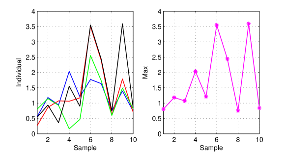
Figure 2: Illustration of the value of code diversity showing the improvement that results from choosing the best of four induced channels.

With sufficient feedback, $|b|\approx 0$, hence $\mathcal{H}^{\dagger}\mathcal{H}\approx\sum_{i=1}^{4}|h_{i}|^{2}\times I_{4}$; therefore, the upper bound for the conditional average pairwise error probability under our code diversity scheme is

$$P_{e|\mathcal{H}}\leq\left(\prod_{i=1}^{4}\omega_{i}\right)^{-1}\left(\frac{E_{s}}{16N_{0}}\right)^{-4}=(\sum_{i=1}^{4}|h_{i}|^{2})^{-4}\left(\frac{E_{s}}{16N_{0}}\right)^{-4}$$ (24)

Since $\mathcal{H}^{\dagger}\mathcal{H}$ is adjusted to have full rank and maximum determinant, the error performance is optimized.

The maximum capacity for the system with four transmit antennas and one receive antenna is

$$\begin{array}[]{ll}C_{0}(4,1)=\mathbf{E}_{H}\log\det\left(I_{1}+\frac{E_{s}}{4N_{0}}HH^{{\dagger}}\right)\\ =\mathbf{E}_{H}\log\det\left(1+\frac{E_{s}}{4N_{0}}\sum_{i=1}^{4}|h_{i}|^{2}\right)\end{array}$$ (25)

The achievable capacity for the QOSTBC under the feedback algorithm can be formulated as

$$\begin{array}[]{ll}C(4,1)=\frac{1}{4}\mathbf{E}_{\mathcal{H}}\log\det\left(I_{4}+\frac{E_{s}}{4N_{0}}\mathcal{H}\mathcal{H}^{{\dagger}}\right)\\ \approx\frac{1}{4}\mathbf{E}_{\mathcal{H}}\log\det\left(I_{4}\times(1+\frac{E_{s}}{4N_{0}}\sum_{i=1}^{4}|h_{i}|^{2})\right)\\ =\mathbf{E}_{\mathcal{H}}\log\det\left(1+\frac{E_{s}}{4N_{0}}\sum_{i=1}^{4}|h_{i}|^{2}\right)\end{array}$$ (26)

Therefore, $C(4,1)\approx C_{0}(4,1)$, i.e.  maximum capacity is closely approached and QOSTBC with code diversity is approximately information lossless.

V-A2 Simulation

The CSI is assumed to be known at the receiver and each channel is modeled as complex Gaussian with zero mean and unit variance. The noise is complex Gaussian with zero mean and unit variance. Then the $\mathop{\mathsf{SNR}}$ is defined as

$$\mathop{\mathsf{SNR}}=\frac{E_{s}}{N_{0}}\frac{\|H\|_{F}^{2}}{4}$$

Where $E_{s}$ is the average transmit symbol power.

Fig. (3) shows the performance improvement through code diversity with two feedback bits (i.e.  $K=4$ for the algorithm described in (23)) using both the ML scheme (15) and the ZF scheme (16) for both 4-QAM and 16-QAM. In the Fig. (3), the prefix ’CD-’ denotes that the corresponding decoding scheme is aided by our code diversity method.

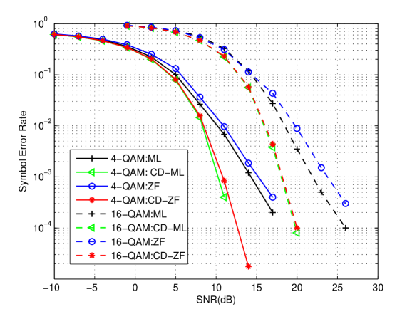
Figure 3: Improvement through Code Diversity for QOSTBC.

The property of quasi-orthogonality implies that the ML scheme has quadratic complexity and the ZF has linear complexity.Two feedback bits improve performance of ML decoding by about $3$ dB for both 4-QAM and 16-QAM. The performance loss from suboptimal zero forcing decoding is minimal.

Remark: Jafarkhani [7] and Su et al. [8] observed that it is possible to achieve full diversity by rotating the signal constellation appropriately. However, the benefits of constellation rotation are limited to small constellations whereas the benefits of code diversity are not. The method of inducing channel phases enlarges the code diversity framework introduced by Tan and Calderbank [9].

V-B Multi-User Detection of Alamouti Signals

Consider a two-user system where each user employs the Alamouti code. The received signals are

$$\begin{array}[]{ll}r_{1}=\mathcal{H}_{1}c_{1}+\mathcal{G}_{1}c_{2}+n_{1}\\ r_{2}=\mathcal{H}_{2}c_{1}+\mathcal{G}_{2}c_{2}+n_{2}\end{array}$$ (27)

where $c_{1}=(x_{1},x_{2})^{T},c_{2}=(x_{3},x_{4})^{T}$ are the signals transmitted by the first and second users respectively. The matrices

$$\begin{array}[]{ll}\mathcal{H}_{1}=\left(\begin{array}[]{cc}h_{11}&h_{21}\\ -h_{21}^{*}&h_{11}^{*}\end{array}\right),\mathcal{G}_{1}=\left(\begin{array}[]{cc}g_{11}&g_{21}\\ -g_{21}^{*}&g_{11}^{*}\end{array}\right)\\ \\ \mathcal{H}_{2}=\left(\begin{array}[]{cc}h_{12}&h_{22}\\ -h_{22}^{*}&h_{12}^{*}\end{array}\right),\mathcal{G}_{2}=\left(\begin{array}[]{cc}g_{12}&g_{22}\\ -g_{22}^{*}&g_{12}^{*}\end{array}\right)\end{array}$$ (28)

are Alamouti blocks, and $H\mathcal{}_{2},\mathcal{G}_{1}$ represent the interference channels.

We can rewrite (27) as

$$\left(\begin{array}[]{c}r_{1}\\ r_{2}\end{array}\right)=\left(\begin{array}[]{cc}\mathcal{H}&\mathcal{G}\end{array}\right)\left(\begin{array}[]{c}c_{1}\\ c_{2}\end{array}\right)+\left(\begin{array}[]{c}n_{1}\\ n_{2}\end{array}\right)$$ (29)

where $\mathcal{H}=(\mathcal{H}_{1},\mathcal{H}_{2})^{T},\;\ \mathcal{G}=(\mathcal{G}_{1},\mathcal{G}_{2})^{T}$.

Several decoding schemes including ML, Bayesian interference cancellation and ZF are explored by Sirianumpiboon et al. [10] where it is shown that

$$\lambda=\frac{\mathcal{H}^{{\dagger}}\mathcal{G}}{\|\mathcal{H}\|\|\mathcal{G}\|}$$ (30)

determines decoding performance.

Take the ZF scheme [17] for example. Setting $W=\left(\begin{array}[]{cc}I_{2}&-\mathcal{G}_{1}\mathcal{G}_{2}^{-1}\\ -\mathcal{H}_{2}\mathcal{H}_{1}^{-1}&I_{2}\end{array}\right)$, we have

$$W\left(\begin{array}[]{c}r_{1}\\ r_{2}\end{array}\right)=\left(\begin{array}[]{cc}\mathcal{H}^{\prime}&0\\ 0&\mathcal{G}^{\prime}\end{array}\right)\left(\begin{array}[]{c}c_{1}\\ c_{2}\end{array}\right)+\left(\begin{array}[]{c}n_{1}^{{}^{\prime}}\\ n_{2}^{{}^{\prime}}\end{array}\right)$$ (31)

where $\mathcal{H}^{\prime}=\mathcal{H}_{1}-\mathcal{G}_{1}\mathcal{G}_{2}^{-1}\mathcal{H}_{2},\;\ \mathcal{G}^{\prime}=\mathcal{G}_{2}-\mathcal{H}_{2}\mathcal{H}_{1}^{-1}\mathcal{G}_{1}$. Thus, $W$ decorrelates two users enabling separate detection. The effective $\mathop{\mathsf{SNR}}$ [10] for the ZF scheme is

$$\frac{\|\mathcal{H}\|\|\mathcal{G}\|}{\sigma^{2}}(1-\|\lambda\|^{2})$$

When $\|\lambda\|=0$, there is no interference and the ZF decoding scheme is optimal.

V-B1 Algorithm Implementation

We use phase adaptation to introduce code diversity so that

$$\begin{array}[]{ll}\mathcal{H}_{1}=\left(\begin{array}[]{cc}h_{11}\gamma_{1}&h_{21}\\ -h_{21}^{*}&h_{11}^{*}\gamma_{1}^{*}\end{array}\right),\mathcal{G}_{2}=\left(\begin{array}[]{cc}g_{12}\gamma_{2}&g_{22}\\ -g_{22}^{*}&g_{12}^{*}\gamma_{2}^{*}\end{array}\right)\\ \\ \mathcal{H}_{2}=\left(\begin{array}[]{cc}h_{12}\gamma_{1}&h_{22}\\ -h_{22}^{*}&h_{12}^{*}\gamma_{1}^{*}\end{array}\right),\mathcal{G}_{1}=\left(\begin{array}[]{cc}g_{11}\gamma_{2}&g_{21}\\ -g_{21}^{*}&g_{11}^{*}\gamma_{2}^{*}\end{array}\right)\end{array}$$ (32)

where $\gamma_{1}=e^{i2\pi\frac{k_{1}}{K_{1}}},\gamma_{2}=e^{i2\pi\frac{k_{2}}{K_{2}}}$; let $K_{1}=K_{2}=4$, corresponding to four bits of feedback. The selection strategy is

$$\{\hat{k_{1}},\hat{k_{2}}\}=\mathop{\rm argmin}_{k_{1}\in\{1,2...,K_{1}\},k_{2}\in\{1,2...,K_{2}\}}\|\lambda\|$$ (33)

V-B2 Simulation

The channels are modeled as complex Gaussian. i.e.

$$\begin{array}[]{ll}h_{11},h_{21},g_{12},g_{22}\sim\mathcal{CN}(0,1)\\ h_{12},h_{22},g_{11},g_{21}\sim\mathcal{CN}(0,\gamma)\end{array}$$ (34)

where the signal to interference ratio $\gamma$ is taken to be $0.5$.

With four bits of feedback i.e.  $K_{1}=K_{2}=4$, the performance of the ML and ZF decoding schemes is shown in Fig. 4 where the prefix ’CD-’ indicates that the corresponding decoding scheme is aided by our code diversity method.

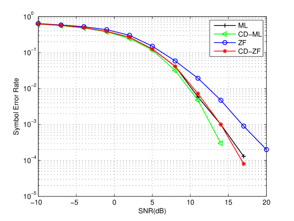
Figure 4: Performance of ZF and ML schemes for Alamouti two-user detection with code diversity for 4-QAM.

Code diversity improves the performance of ZF decoding by more than $2$ dB and matches the performance of ML decoding. The performance of ML decoding is also improved by approximately $1$ dB.

V-C Code Diversity for the Golden Code

Here code diversity is implemented by switching between equivalent variants of the Golden code.

V-C1 Equivalent Variants of Golden Code

We recall the structure of the Golden code [12, 13, 14] as

$$G_{1}=\left(\begin{array}[]{cc}s_{1}+\tau s_{2}&s_{3}+\tau s_{4}\\ i(s_{3}+\mu s_{4})&s_{1}+\mu s_{2}\end{array}\right)$$ (35)

where $\tau=\frac{1+\sqrt{5}}{2}$ and $\mu=\frac{1-\sqrt{5}}{2}$.

Switching the positions of $\tau$ and $\mu$ yields the variant

$$G_{2}=\left(\begin{array}[]{cc}s_{1}+\mu s_{2}&s_{3}+\mu s_{4}\\ i(s_{3}+\tau s_{4})&s_{1}+\tau s_{2}\end{array}\right)$$ (36)

V-C2 $2\times 1$ systems

Let $h_{1}$ and $h_{2}$ be channel gains from the two transmit antennas to the single receive antenna which are modeled as Rayleigh $h_{i}\sim\mathcal{CN}(0,\sigma^{2}),i=1,2$. The noise is complex gaussian as $\mathcal{CN}(0,N_{0})$ and $\mathsf{SNR}$ is defined as

$$\mathsf{SNR}=\frac{E_{s}\sigma^{2}\left(2+\tau^{2}+\mu^{2}\right)}{N_{0}}$$ (37)

where $E_{s}$ is the average transmitting signal power.

Given $h_{1}$ and $h_{2}$, the instantaneous $\mathsf{SNR}$ for code $G_{1}$ is

$$S_{1}=\frac{E_{s}\{|h_{1}|^{2}(1+\tau^{2})+|h_{2}|^{2}(1+\mu^{2})\}}{N_{0}}$$

and the instantaneous $\mathsf{SNR}$ for code $G_{2}$ is

$$S_{2}=\frac{E_{s}\{|h_{1}|^{2}(1+\mu^{2})+|h_{2}|^{2}(1+\tau^{2})\}}{N_{0}}.$$

We observe $S_{1}>S_{2}$ if and only if $|h_{1}|>|h_{2}|$.

Our code diversity scheme is to select $G_{1}$ if $S_{1}>S_{2}$ otherwise to select $G_{2}$. Code diversity improves the average $\mathsf{SNR}$ to

$$S_{CD}=\frac{E_{s}\{\mathbf{E}[h_{max}^{2}](1+\mu^{2})+\mathbf{E}[h_{min}^{2}](1+\tau^{2})\}}{N_{0}}$$ (38)

where $h_{max}=\max\{|h_{1}|,|h_{2}|\},h_{min}=\min\{|h_{1}|,|h_{2}|\}$.
Proposition 1: Given Rayleigh channel gains ($f_{|h_{i}|}(x)=\frac{x}{\sigma^{2}}e^{-\frac{x^{2}}{2\sigma^{2}}},i=1,2$), the above form of code diversity improves the performance of ML decoding of the Golden code by $0.88$ dB.
Proof: The distribution function for $|h_{i}|$ is $f_{|h_{i}|}(x)=\frac{x}{\sigma^{2}}e^{-\frac{x^{2}}{2\sigma^{2}}},i=1,2$ and the accumulative distribution function is $F_{|h_{i}|}(x)=1-e^{-\frac{x^{2}}{2\sigma^{2}}}$. Therefore the distribution function of $h_{max}=\max\{|h_{1}|,|h_{2}|\}$ is given by

$$\begin{array}[]{ll}f_{max}(x)=\frac{d\{F_{|h_{1}|}(x)F_{|h_{2}|}(x)\}}{dx}\\ \hskip 38.41121pt=\frac{dF^{2}_{|h_{i}|}(x)}{dx}=\frac{2x}{\sigma^{2}}\left(e^{-\frac{x^{2}}{2\sigma^{2}}}-e^{-\frac{x^{2}}{\sigma^{2}}}\right),\end{array}$$ (39)

hence $\mathbf{E}[h_{max}^{2}]=1.5\sigma^{2}$.

The distribution function of $h_{min}=\min\{|h_{1}|,|h_{2}|\}$ is given by

$$\begin{array}[]{ll}f_{min}(x)=\frac{d\left(1-F_{|h_{1}|}(x)\right)\left(1-F_{|h_{2}|}(x)\right)}{dx}\\ \hskip 35.56593pt=\frac{2x}{\sigma^{2}}e^{-\frac{x^{2}}{\sigma^{2}}},\end{array}$$ (40)

hence $\mathbf{E}[h_{min}^{2}]=0.5\sigma^{2}$.

The gain is given by

$$\begin{array}[]{ll}G_{1rx}=10\log(\frac{S_{CD}}{\mathsf{SNR}})\\ =10\log\frac{\mathbb{E}[h_{max}^{2}](1+\mu^{2})+\mathbb{E}[h_{min}^{2}](1+\tau^{2})\}}{\sigma^{2}\left(2+\tau^{2}+\mu^{2}\right)}=0.88\;\ dB\end{array}$$ (41)

$\square$

V-C3 $2\times 2$ systems

Let $h_{1},h_{2}$ be channel gains from the two transmit antennas to the first receive antenna and $h_{3},h_{4}$ for the second receive antenna. The $\mathsf{SNR}$ is the same as defined in (37).

For $G_{1}$, the instantaneous $\mathsf{SNR}$ is

$$S_{1}=\frac{E_{s}\{(|h_{1}|^{2}+|h_{3}|^{2})(1+\tau^{2})+(|h_{2}|^{2}+|h_{4}|^{2})(1+\mu^{2})\}}{2N_{0}}$$

For $G_{2}$, the instantaneous $\mathsf{SNR}$ is

$$S_{2}=\frac{E_{s}\{(|h_{1}|^{2}+|h_{3}|^{2})(1+\mu^{2})+(|h_{2}|^{2}+|h_{4}|^{2})(1+\tau^{2})\}}{2N_{0}}$$

and we observe

$$S_{1}>S_{2}\iff|h_{1}|^{2}+|h_{3}|^{2}>|h_{2}|^{2}+|h_{4}|^{2}.$$

Code diversity is implemented by selecting $G_{1}$ if $S_{1}>S_{2}$ otherwise selecting $G_{2}$. Monte Carlo simulation shows that under code diversity, the gain over ML decoding error performance is

$$G_{2rx}=0.66\;\ dB$$ (42)

V-C4 Simulations

The simulations shown in Fig. 5 employ a single feedback bit. Performance is improved by about $1$ dB for $2\times 1$ systems and about $0.5$ dB for $2\times 2$ systems; the simulation result is consistent with the analysis.

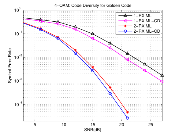
Figure 5: Improvement to the ML Decoder for the Golden code through Code Diversity.

VI A family of Full Rate Circulant Code Designs based on Code Diversity

Observing the rarity of full rate $M\times M$ code designs as $M$ becomes relatively large, we propose a family of full rate codes based on circulant matrix in this section. Code designs based on circulant matrix without feedback are studied. We also illustrate a universal linear decoder using Fourier basis for the family of circulant codes within the code diversity framework.

VI-A Circulant Matrices and Their Properties

An $M\times M$ circulant matrix takes the form

$$X=\left(\begin{array}[]{c}\vec{x}\\ \vec{x}L\\ \cdots\\ \vec{x}L^{M-1}\end{array}\right)$$ (43)

where $\vec{x}=(x_{1},x_{2},\cdots,x_{M})$ and $(x_{1},x_{2},\cdots,x_{M})L=(x_{M},x_{1},\cdots,x_{M-1})$. We recall the following properties of circulant matrices and refer the reader to [24] for more details.
Lemma 1: Let $\omega=e^{\frac{2\pi i}{M}}$. The eigenvectors of the shift operator L are the Fourier basis $f_{j}=(1,\omega^{j},\omega^{2j},\cdots,\omega^{(M-1)j})^{T},j=0,1,\cdots,M-1$ and $Lf_{j}=\omega^{j}f_{j}$.
Lemma 2: A matrix $X$ commutes with the left shift matrix $L$ if and only if $X$ is a circulant matrix.
Property 1: Let $X$ be an $M\times M$ circulant design. Then the Fourier basis $F=\{f_{0},\cdots,f_{M-1}\}$ is an orthogonal set of eigenvectors of $X$.
Proof: We have $L(Xf_{j})=XLf_{j}=\lambda_{j}(L)Xf_{j},j=0,1,\cdots,M-1$ and so $Xf_{j}$ is a multiple of $f_{j}$.$\square$
Property 2: Let $X$ be an $M\times M$ circulant design with first row $\vec{x}$. Then the $j^{th}$ eigenvalue of $X$ is $\lambda_{j}(X)=\vec{x}f_{j}$.
Proof:

$$\begin{array}[]{ll}Xf_{j}=\left(\begin{array}[]{c}\vec{x}\\ \vec{x}L\\ \cdots\\ \vec{x}L^{M-1}\end{array}\right)f_{j}=\left(\begin{array}[]{c}\vec{x}f_{j}\\ \vec{x}Lf_{j}\\ \cdots\\ \vec{x}L^{M-1}f_{j}\end{array}\right)\\ \\ =\vec{x}f_{j}\left(\begin{array}[]{c}1\\ \omega^{j}\\ \cdots\\ \omega^{(M-1)j}\end{array}\right)=(\vec{x}f_{j})f_{j}\end{array}$$ (44)

therefore, $\lambda_{j}(X)=\vec{x}f_{j}$. $\square$

VI-B $3\times 3$ Circulant Design without Feedback

Consider the $3\times 3$ circulant code $C$ given by

$$C=\left(\begin{array}[]{ccc}x_{1}\alpha&x_{2}\beta&x_{3}\\ x_{2}\beta&x_{3}&x_{1}\alpha\\ x_{3}&x_{1}\alpha&x_{2}\beta\end{array}\right)$$ (45)

where $\alpha=(\frac{1+\sqrt{5}}{2})^{\frac{1}{3}}$, $\beta=(\frac{1-\sqrt{5}}{2})^{\frac{1}{3}}$ and $x_{i}$ are symbols from QAM constellation.

VI-B1 Full Rate

This $3\times 3$ circulant design is full rate since it transmits three symbols over three consecutive time slots.

VI-B2 Full Diversity

Consider two distinct codewords $C_{1}$ and $C_{2}$ with symbols on QAM constellation. Then,

$$|det(C_{1}-C_{2})|=\left|\frac{1+\sqrt{5}}{2}s_{1}^{3}+\frac{1-\sqrt{5}}{2}s_{2}^{3}+s_{3}^{3}+3s_{1}s_{2}s_{3}\right|$$

where $s_{i},i=1,2,3$ are the corresponding symbol differences and $s_{i}$ are gaussian integers.

• if $s_{1}\neq s_{2}$, then $C_{1}-C_{2}$ is irrational and so $|det(C_{1}-C_{2})|\neq 0$.

• if $s_{1}=s_{2}$, then $|det(C_{1}-C_{2})|=0$ if and only if $s_{1}^{3}+s_{3}^{3}+3s_{1}^{2}s_{3}=0$. Since $z^{3}+3z+1=0$ has no solution in $Q(i)$, so $s_{1}^{3}+s_{3}^{3}+3s_{1}^{2}s_{3}=0$ has no solution in $Z(i)$. Therefore, $|det(C_{1}-C_{2})|\neq 0$.

Hence, it has full diversity.

VI-B3 Simulation

We compare this $3\times 3$ circulant code with the Alamouti code at the same transmission rate of two bits per time slot in Fig. 6 (both using 4-QAM signaling). The $3\times 3$ circulant code outperforms the Alamouti code significantly and has a larger diversity which is indicated by the slope of the curves.

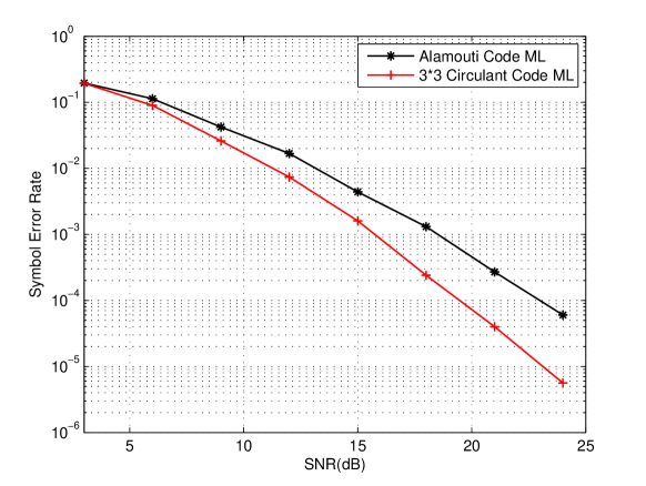
Figure 6: Performance comparison of the $3\times 3$ circulant code with the Alamouti code. Curvers are for ML decoding and $4-$QAM signaling.

Remark: General $M\times M$ circulant codes can be produced using similar techniques.

VI-C Integration of Circulant Codes and Code Diversity

With code diversity, we use circulant matrix in (43) or their variants such as the one in (45) as our coding block. We observe that the circulant structure transfers from the transmitter to the receiver (of (2)), in that the received signal $r$ can be written as

$$r=\mathcal{H}c+n$$ (46)

where $c=(x_{1},x_{2},\cdots,x_{M})^{T}$, $x_{i}$ is taken from certain constellations, $n$ is the corresponding additive noise and

$$\mathcal{H}=\left(\begin{array}[]{c}\vec{h}\\ \vec{h}L\\ \cdots\\ \vec{h}L^{M-1}\end{array}\right)$$ (47)

where $\vec{h}=(h_{1},h_{2},\cdots,h_{M})$ with $h_{j}$ as the channel gain between the $j^{th}$ transmit antenna and the single receive antenna.

VI-C1 Code Diversity Algorithm

We modify the phase of the channel gain $h_{1}$ as follows:

$$\begin{array}[]{ll}\hat{k}=\mathop{\rm argmax}_{k\in K}det(\mathcal{H}^{{\dagger}}\mathcal{H})|_{h_{1}\rightarrow h_{1}e^{\frac{ik\pi}{K}}}\\ \\ \hskip 14.22636pt=\mathop{\rm argmax}_{k\in K}\left|\prod^{N}_{j=1}\vec{h}f_{j}\right|_{h_{1}\rightarrow h_{1}e^{\frac{ik\pi}{K}}}\end{array}$$ (48)

where $\log_{2}K$ is the number of feedback bits. More channel gains may need to be modified as $M$ increases.

VI-C2 Linear decoder based on Fourier Basis

From equation (46), we have

$$F^{-1}r=F^{-1}\mathcal{H}FF^{-1}c+F^{-1}n$$ (49)

and we observe that $F^{-1}=\frac{1}{M}F^{\prime}$, where $F^{\prime}$ is the entry-wise conjugate of $F$, so we get

$$F^{\prime}r=\Lambda_{\mathcal{H}}F^{\prime}c+F^{\prime}n$$ (50)

where $\Lambda_{\mathcal{H}}=F^{-1}\mathcal{H}F=\mathsf{diag}\{\vec{h}f_{0},\cdots,\vec{h}f_{M-1}\}$. We also observe that $f_{j}^{T}F^{\prime}c=Mx_{j},\forall j=1,\cdots,M$.

We propose the linear decoder as

$$\hat{x}_{j}=\mathop{\rm argmin}_{x_{j}\in\mathbb{C}}\left|\frac{1}{M}f_{j}^{T}\Lambda^{-1}_{\mathcal{H}}F^{\prime}c-x_{j}\right|^{2}$$ (51)

The decoding performance of the linear decoder mainly depends on $\det{\Lambda_{\mathcal{H}}}$ which is exactly $(\det{\mathcal{H}^{{\dagger}}\mathcal{H}})^{\frac{1}{2}}$. Our code diversity algorithm precisely aims to raise $\det{\mathcal{H}^{{\dagger}}\mathcal{H}}$. Therefore, the performance of the linear decoder is guaranteed within the code diversity framework.

VII Conclusion

We have introduced a general information theoretic framework for the analysis of code diversity. we have shown that it not only improves the diversity and coding advantages for general space time codes but enables optimal decoding performance with low complexity decoding and only a small number of feedback bits. The method of code diversity also reduces the capacity loss associated with some forms of space-time coding. We have also proposed a family of full rate circulant code designs based on code diversity and a corresponding universal linear decoding algorithm using decomposition of circulant matrices. An extensive study of $3\times 3$ circulant design shows that it outperforms the Alamouti code at the same transmission rate.

VIII Acknowledgement

The authors would like to thank Chee Wei Tan for many helpful suggestions and for bringing the work of Bonnet et al. to their attention.

References

• [1] V. Tarokh, N. Seshadri and A. R. Calderbank, β€œSpace time codes for high data rate wireless communication: Performance analysis and code construction,” IEEE Transactions on Information Theory, vol. 44, pp. 744-765, March 1998.
• [2] V. Tarokh, H. Jafarkhani and A. R. Calderbank, β€œSpace-time block codes from orthogonal designs,” IEEE Transactions on Information Theory, vol. 45, pp. 1456-1467, July 1999.
• [3] F. Oggier, G. Rekaya, J.-C. Belfiore and E. Viterbo, β€œPerfect space-time block codes,” IEEE Transactions on Information Theory, vol. 52, pp. 3885-3902, September 2006.
• [4] I. E. Telatar, β€œCapacity of multi-antenna Gaussian channels,” European Transactions on Communications, vol. 10, pp. 585-595, November 1999.
• [5] B. Hassibi and B. M. Hochwald, β€œHigh-rate codes that are linear in space and time,” IEEE Transactions on Information Theory, vol. 48, No. 7, pp. 1804-1824, July 2002.
• [6] H. Jafarkhani, β€œA quasi-orthogonal space-time block code,” IEEE Transactions on Communications, vol. 49, pp. 937-950, January 2003.
• [7] H. Jafarkhani, Space-time coding: Theory and practice, Cambridge University Press, 2005.
• [8] W. Su and X.-G. Xia, β€œSignal constellations for quasi-orthogonal space-time block codes with full diversity,” IEEE Transactions on Information Theory, vol. 50, pp. 2331-2347, October 2004.
• [9] C. W. Tan and A. R. Calderbank, Multiuser Detection of Alamouti Signals, submitted to IEEE Trans. of Communications, November 2007. This work has also appeared at Princeton University, Sup lec and Alcatel-Lucent Bell Labs Workshop On Wireless Communications and Networks.
• [10] S. Sirianunpiboon, A. R. Calderbank and S. D. Howard, β€œSpace-polarization-time codes for diversity gains across line of sight and rich scattering Environments,” in Proc. IEEE ITW, May 2007.
• [11] M. O. Damen, A. Tewfik and J.-C. Belfiore, β€œA construction of a space-time code based on number theory,” IEEE Transactions on Information Theory, Vol. 48, pp. 753-760, March 2002.
• [12] J.-C. Belfiore, G. Regaya, and E. Viterbo, β€œThe golden code: A $2\times 2$ full-rate space-time code with nonvanishing determinants,”, IEEE Transactions on Information Theory, Vol. 51, pp. 1432-1436, April 2005.
• [13] H. Yao and G. W. Wornell, β€œAchieving the full MIMO diversity multiplexing frontier with rotation-based space-time codes,” in Proc. Allerton Conference on Communication, control and Computing, October 2003.
• [14] P. Dayal and M. K. Varanasi, β€œOptimal two transmit antenna space-time code and its stacked extensions,” IEEE Transaction on Information Theory, Vol. 49, pp. 1073-1096, May 2003.
• [15] P. Viswanath, D. David N.C. Tse and Rajiv Laroia, β€œOpportunistic beamforming using dumb antennas,” IEEE Transactions on Information Theory, vol. 48, no. 6, pp. 1277-1294, June 2002.
• [16] J. JaldΓ©n and B. Ottersten, β€œOn the complexity of sphere decoding in digital communications,” IEEE Transactions on Signal Processing, vol. 53, pp. 1474-1484, April 2005.
• [17] A. F. Naguib and N. Seshadri, β€œ Combined interference cancellation and ML decoding of space-time block codes,” in Proc. Comm. Theory Minicomference, held in conjunction with Globecomm’98, (Sydney, Australia), pp. 7-15, 1998.
• [18] C. Lin, V. Raghavan and V. V. Veeravalli, β€œTo code or not to code across time: space-time coding with feedback,” Submitted to the IEEE Journal on Selected Areas in Communication, November 2007.
• [19] J. Bonnet, O. Tirkkonen and A. Hottinen, β€œClosed-loop modes for two high-rate linear space-time block codes,” in Proc. IEEE ICC 2005, (Seoul Korea), May 2005.
• [20] G. Bresler and B. Hajek, β€œNote on mutual information and orthogonal space-time codes,” ISIT 2008, Seattle, July, 2006.
• [21] A. R. Calderbank and A. F. Naguib. Orthogonal designs and third generation wireless communication, Surveys in Combinatorics 2001, pp. 75-107, edited by J. W. P. Hirschfeld, London Math. Soc. Lecture Note Series 288, Cambridge Univ. Press, 2001.
• [22] W. Wolfe, Amicable orthogonal designs - Existence, Canadian J. Math., vol. 28, pp. 1006-1020, 1976.
• [23] X-B. Liang, β€œOrthogonal designs with maximal rates,” IEEE Transactions on Information Theory, vol. 49, pp. 2468-2503, October 2003.
• [24] P. J. Davis, Circulant matrices, John Wiley $\&$ Sons, 1979.
• [25] A. Hottinen and O. Tirkkonen, β€œPrecoder designs for high rate space-time block codes,” in Proc. Conference on Informatiion Sciences and Systems, Princeton, March 2004.
• [26] A. Hottinen, K. Kuchi and O. Tirkkonen, β€œA space-time coding concept for a multi-antenna transmitter,” in Proc. Canadian Workshop on Information Theory, Vancouver, June 2001.
• [27] A. Hottinen, O. Tirkkonen and R. Wichman, β€œMulti-antenna transceiver techniques for 3G and beyond,” WILEY publisher, UK, March 2003.
• [28] O. Tirkkonen and A. Hottinen, β€œSquare-matrix embeddable space-time block codes for complex signal constellations,” IEEE Transaction on Information Theory, vol. 48, no. 2, pp. 384-395, February 2002.
• [29] O. Tirkkonen and R. Kashaev, β€œCombined information and performance optimization of linear MIMO modulations,” in IEEE ISIT 2002, Lausanne, Switzerland, p. 76, June 2002.
• [30] J. Paredes, A. B. Gershman, and M. G. Alkhanari, β€œA $2\times 2$ space-time code with non-vanishing determinants and fast maximum likelihood decoding,” in IEEE ICASSP 2007, Honolulu, Hawaii, USA, pp. 877-880, April 2007.