A Search for the Most Massive Galaxies. II.
Structure, Environment and Formation

Abstract

We study a sample of 43 early-type galaxies, selected from the Sloan Digital Sky Survey (SDSS) because they appeared to have velocity dispersions of $\sigma\geq$350 kms^-1. High-resolution photometry in the SDSS $i$ passband using the High-Resolution Channel of the Advanced Camera for Surveys on board the Hubble Space Telescope shows that just less than half of the sample is made up of superpositions of two or three galaxies, so the reported velocity dispersion is incorrect. The other half of the sample is made up of single objects with genuinely large velocity dispersions. None of these objects has $\sigma$ larger than $426\pm 30$ km s^-1. These objects define rather different size-, mass- and density-luminosity relations than the bulk of the early-type galaxy population: for their luminosities, they are the smallest, most massive and densest galaxies in the Universe. Although the slopes of the scaling relations they define are rather different from those of the bulk of the population, they lie approximately parallel to those of the bulk at fixed $\sigma$. This suggests that these objects are simply the large-$\sigma$ extremes of the early-type population – they are not otherwise unusual. These objects appear to be of two distinct types: the less luminous ($M_{r}>-23$) objects are rather flattened, and their properties suggest some amount of rotational support. While this may complicate interpretation of the SDSS velocity dispersion estimate, and hence estimates of their dynamical mass and density, we argue that these objects are extremely dense for their luminosities, suggesting merger histories with abnormally large amounts of gaseous dissipation. The more luminous objects ($M_{r}<-23$) tend to be round and to lie in or at the centers of clusters. Their circular isophotes, large velocity dispersions, and environments are consistent with the hypothesis that they are BCGs. Models in which BCGs form from predominantly radial mergers having little angular momentum predict that they should be prolate. If viewed along the major axis, such objects would appear to have abnormally large velocity dispersions for their sizes, and to be abnormally round for their luminosities. This is true of the objects in our sample once we account for the fact that the most luminous galaxies ($M_{r}<-23.5$), and BCGs, become slightly less round with increasing luminosity. Thus, the shapes of the most luminous galaxies suggest that they formed from radial mergers, and the shapes of the most luminous objects in our big-$\sigma$ sample suggest that they are the densest of these objects, viewed along the major axis.

1 Introduction

The most massive galaxies may place interesting constraints on models of galaxy formation (e.g. De Lucia et al. 2006; Almeida et al. 2007). But which observable one should use as a proxy for mass is debatable. If luminosity is a good proxy, then the Brightest Cluster Galaxies should be the most massive galaxies; this has led to considerable interest in their properties (Scott 1957; Sandage 1976; Thuan & Romanishin 1981; Malumuth & Kirschner 1981; Hoessel et al. 1987; Schombert 1987, 1988; Oegerle & Hoessel 1991; Lauer & Postman 1994; Postman & Lauer 1995; Crawford et al. 1999; Laine et al. 2003; Lauer et al. 2007; Bernardi et al. 2007a).

Figure 1: Surface brightness isophotes of the objects in our sample, which provide the basis for determining which objects are singles. The two panels for each object show a larger $5\times 5$ arcsec region with logarithmically spaced isophotes, and a $1\times 1$ arcsec region with linearly spaced isophotes. Thick solid circle shows the size of the SDSS fiber; structure within this circle is likely to have contributed to the estimated velocity dispersion, whereas structures outside it have not.

Figure 2: Continued from previous figure. The assymetry in in the image which is second from top on the right is due to dust.

Figure 3: Continued from previous figure.

Figure 4: Continued from previous figure.

Figure 5: Continued from previous figure.

Figure 6: Continued from previous figure.

However, velocity dispersion is sometimes used as a surrogate for mass (the virial theorem has mass $\propto R\sigma^{2}$), so it is interesting to ask if a sample selected on the basis of velocity dispersion also contains the most massive galaxies. Such a sample is also interesting in view of the fact that black hole mass correlates strongly and tightly with velocity dispersion (Ferrarese & Merritt 2000; Gebhardt et al. 2000), so galaxies with large $\sigma$ are expected to host the most massive black holes.

With this in mind, Bernardi et al. (2006) culled a sample of $\sim 100$ objects with $\sigma>350$ km s^-1 from the First Data Release of the Sload Digital Sky Survey (SDSS DR1; Abazajian et al. 2003). The total area from which these objects were selected is about 2000 deg²; for a spatially flat Universe with $\Omega_{m}=0.3$ and Hubble constant $H_{0}=70$ km s^-1, which we assume in what follows, this corresponds to a comoving volume of about $3.34\times 10^{8}$ Mpc³ out to $z=0.3$.

Some of these objects turned out to be objects in superposition, evidence for which came primarily from the spectra (see Bernardi et al. 2006 for details). A random subset of the others, 43 objects in all, was observed with the High Resolution Camera of the Advanced Camera System on board the Hubble Space Telescope (HST-ACS HRC). On the basis of this high-resolution imaging, we have been able to separate out the true singles from those which are objects in superposition. As a result, we are now able to study the properties of objects with large $\sigma$.

We describe the HST observations, our identification of the truly single objects, our classification of their isophotal shapes, and how we combine the HST imaging with SDSS data to determine the environments of these objects in Section 2. The isophotal shapes of these objects are compared with those of BCGs in Section 3. Various scaling relations, size-luminosity, the fundamental plane, etc. are presented in Section 4. While these relations are different from those defined by the bulk of the early-type galaxy population, we show that they can actually be derived from the early-type scaling relations simply by studying what these relations look like at fixed velocity dispersion. These analyses show that our sample appears to contain two distinct types of objects: the more luminous objects tend to be round, have large sizes as well as velocity dispersions, and tend to be in crowded fields. Indeed, they are rounder than other objects of similar luminosities, so it is possible that they are prolate, and viewed along the long axis. The less luminous objects are not round, have abnormally small sizes and are not necessarily in crowded fields; even if rotational motions have compromised the SDSS velocity dispersion estimates, these objects may be amongst the densest galaxies for their luminosities. A final section summarizes our findings and discusses some implications of the bimodal distribution we have found, as well as of the fact that no galaxy appears to have a velocity dispersion larger than $426\pm 30$ km s^-1.

In a companion paper (Hyde et al. 2008), we study the surface brightness profiles of the objects classified as singles in much more detail, placing them in the context of other HST-based studies of early-type galaxies (e.g. Laine et al. 2003; Ferrarese et al. 2006; Lauer et al. 2007).

2 The data

2.1 HST Observations

The analysis below is based on observations taken between August 2004 and June 2005 as part of a Cycle 13 Snapshot Survey. The target list for the Snapshot Survey contained 70 objects, all of which were selected from the SDSS as described in Paper I; i.e., they all had reported velocity dispersions larger than 350 km s^-1, and none were identified from the imaging, the line profiles or the cross-correlation analyses described in Paper I as being multiple. Of these 70 objects, 43 were observed.

The following observing sequence was adopted for each target galaxy:
-The center of each galaxy was positioned close to the HRC aperture.
-A total integration time of 1200 s in the F775W (which resembles SDSS $i$) filter, split into four exposures of 300 s, was used.
-Each visit used the line-dither pattern to allow removal of most cosmic ray events.
Data reduction details and analysis of the photometric profiles are presented in Hyde et al. (2008).

2.2 Identifying the singles

In the present context, the great virtue of HST is its angular resolution ($\sim 0.025$ arcsec/pixel): at the median redshift of our sample, $z=0.24$, scales down to about 95 pc are resolved. (This scale, for SDSS imaging, is about sixty times larger.) Therefore, a simple visual inspection of the F775W images allowed a classification into three groups:
(i) 23 targets showed no evidence for superposition - we call these single galaxies;
(ii) 15 targets appear to be superpositions of two galaxies - we call these doubles;
(iii) 5 targets show evidence for more than two components - we call these multiples.

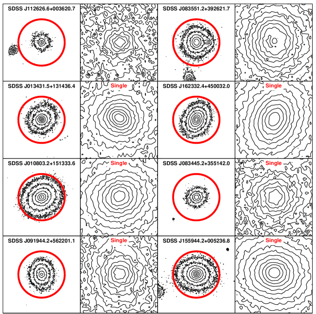
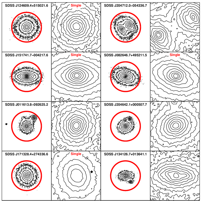
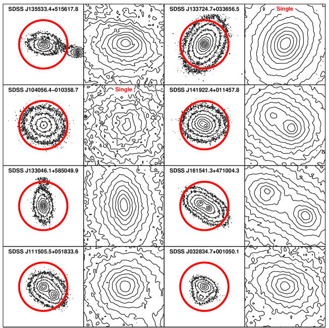
Figures 1–6 show density contours (isophotes) obtained from the ACS F775W images of these objects. Two panels are shown for each object. The panels on the left show fields-of-view that are approximately $5\times 5$ arcsec² (North is up, East is to the left), and the contours are linearly spaced in magnitude (logarithmically spaced in flux). The solid circle shows the angular size of the SDSS fiber (3 arcsec in diameter). This is the scale within which the velocity dispersion was measured (this measured value is aperture corrected to $R_{e}/8$ - see Bernardi et al. 2006 for details). Light from objects outside the circle is very unlikely to affect the velocity dispersion and absorption line-index measurements. The panels on the right show the central arcsecond, and the contours are linearly spaced in flux. In these panels, we specify if the object was classified as a single. These figures illustrate that the classification into singles, doubles and multiples is relatively straightforward. Table 1 provides details of these classifications.

Figure 7: Velocity dispersions of early-type galaxies in our sample sample as a function of redshift. Circles represent the singles, squares show the doubles, and squares with an additional cross show objects which are superpositions of more than two components. Small filled squares show objects which Bernardi et al. (2006) thought were likely to be massive single galaxies. We only show measurement uncertainties on the singles; uncertainties on the other objects are similar, although the systematic error is, of course, substantially larger.

Table 1: The 43 objects with velocity dispersions larger than 350 km s^-1 from Bernardi et al. (2006) which have HST images. ID_S identifies the single objects whose properties are given in Table 2. N_objs gives the number of objects inside a circle of 3 arcsec in diameter. Env = 0,1 means low-, high-density (see text for details). Prof = c,p,d means core, power-law, obvious presence of dust (from Hyde et al. 2008).

Name	IDS	Nobjs	Env	Prof
SDSS J112626.6$+$003620.7	–	2	0	–
SDSS J083551.2$+$392621.7	–	3	1	–
SDSS J013431.5$+$131436.4	1	1	0	p
SDSS J162332.4$+$450032.0	2	1	1	c
SDSS J010803.2$+$151333.6	3	1	0	c
SDSS J083445.2$+$355142.0	4	1	1	c
SDSS J091944.2$+$562201.1	5	1	1	c
SDSS J155944.2$+$005236.8	6	1	0	c
SDSS J135602.4$+$021044.6	7	1	1	c
SDSS J075923.1$+$274148.3	–	2	1	–
SDSS J141341.4$+$033104.3	8	1	0	c
SDSS J112842.0$+$043221.7	9	1	0	p,d
SDSS J124134.3$+$604147.2	–	2	0	–
SDSS J093124.4$+$574926.6	10	1	0	p
SDSS J103344.2$+$043143.5	11	1	0	p,d
SDSS J221414.3$+$131703.7	12	1	0	p
SDSS J120011.1$+$680924.8	13	1	1	c
SDSS J211019.2$+$095047.1	14	1	1	c
SDSS J160239.1$+$022110.0	15	1	1	p
SDSS J154017.3$+$430024.5	–	2	1	–
SDSS J111525.7$+$024033.9	16	1	0	p
SDSS J145506.8$+$615809.7	–	2	1	–
SDSS J235354.1$-$093908.3	–	2	0	–
SDSS J082216.5$+$481519.1	17	1	0	p,d
SDSS J124609.4$+$515021.6	18	1	1	c
SDSS J204712.0$-$054336.7	–	3	1	–
SDSS J151741.7$-$004217.6	19	1	1	p
SDSS J082646.7$+$495211.5	20	1	0	p,d
SDSS J011613.8$-$092625.2	–	2	0	–
SDSS J204642.1$+$000507.7	–	3	1	–
SDSS J171328.4$+$274336.6	21	1	1	c
SDSS J134126.7$+$013641.1	–	3	0	–
SDSS J135533.4$+$515617.8	–	2	0	–
SDSS J133724.7$+$033656.5	22	1	1	c
SDSS J104056.4$-$010358.7	23	1	1	c
SDSS J141922.4$+$011457.8	–	2	1	–
SDSS J133046.1$+$585049.9	–	2	0	–
SDSS J161541.3$+$471004.3	–	2	1	–
SDSS J111505.5$+$051833.6	–	2	0	–
SDSS J032834.7$+$001050.1	–	2	0	–
SDSS J010354.1$+$144814.1	–	2	0	–
SDSS J114747.0$+$034838.7	–	2	0	–
SDSS J104940.3$+$050307.1	–	2	1	–

Finally, note that a few of the objects in this sample (SDSS J103344.2$+$043143.5, SDSS J112842.0+043221.7, SDSS J082646.7+495211.5 and SDSS J082216.5+481519.1) show clear evidence for dust; this is studied in more detail in Hyde et al. (2008).

Figure 8: Normalized distribution of SDSS early-type velocity dispersions before and after removing the contribution from objects which are superpositions. Filled circles with error bars show the measured distribution with no correction (other than to account for the apparent magnitude limit by weighting each object by $1/V_{\rm max}$); open symbols show the result of removing superpositions on the basis of SDSS imaging or spectra (e.g. following Bernardi et al. 2006) - since this does not find all the superpositions, this will overestimate the true abundance; and filled circles without error bars show the result of assuming that the only singles are those identified by HST - since this incorrectly assumes that all the others are superpositions, it underestimates the true abundance. Smooth curves show fits to the functional form given by Sheth et al. (2003); the curve which predicts lower abundances at large $\sigma$ is an estimate of the intrinsic distribution. Convolving it with measurement errors yields the other curve.

2.3 Parameters from SDSS images and spectra

The SDSS imaging reductions are known to suffer from sky subtraction problems, particularly for large objects. To address this problem, for the sample of large velocity dispersion galaxies, we have recomputed the photometric parameters (i.e. deVaucouleur magnitudes, sizes, $b/a$ and model color) from the SDSS r-band images using GalMorph (Hyde et al. 2008). The photometric parameters of the entire SDSS early-type sample were corrected following equations (1-4) of Hyde & Bernardi (2008). The spectroscopic parameters, velocity dispersions and Mg₂ index-strengths for the objects with $\sigma>350$ km s^-1 are from Bernardi et al. (2006); those for the rest of the early-type sample are from DR6 (since these do not suffer from the bias at small $\sigma$ that is present in previous SDSS data releases – see DR6 documentation and Bernardi 2007). Table 2 lists the parameters used in this work. A more extensive analysis of the HST (rather than SDSS) surface brightness profiles of these objects is provided by Hyde et al. (2008).

2.4 The environments of these objects

In most of the analysis which follows, the environment of these objects is irrelevant. However, whether or not the objects with the largest velocity dispersions are preferentially found in dense environments is an interesting question. This is because, in hierarchical models, the most massive halos are predicted to populate the densest regions (Mo & White 1996; Sheth & Tormen 2002), a trend for which there is good observational evidence (e.g. Abbas & Sheth 2007). Massive halos are expected to host the most massive galaxies (e.g. De Lucia et al. 2006; Almeida et al. 2007), so if the largest velocity dispersions reflect large masses, then one expects a correlation between $\sigma$ and environment. One might also wish to check if the objects which are superpositions are found in particularly crowded fields. To briefly address these questions, we have made a rough estimate of the environment of each object as follows.

From the SDSS DR5, we select fields which are approximately 1 Mpc $\times$ 1 Mpc centred on each target. For the most distant objects in our sample ($z\sim 0.3$), the fields are about $3^{\prime}\times 3^{\prime}$, whereas they are about $9^{\prime}\times 9^{\prime}$ for the closest objects ($z\sim 0.1$). The SDSS provides photometric information (colors, photometric redshifts) for all the objects in the field which are brighter than about $m_{r}=22.5$. If spectroscopic information is also available (in general, if $m_{r}$ is brighter than $\sim 17.5$), we count the object as a neighbour if it lies within 3000 km s^-1 of the target. If only photometry is available, an object counts as a neighbour if the photometric redshift is within 7500 km s^-1 of the target. We then classify the targets as being in group or cluster like environments if the number of neighbours is greater than 30. (Changing this threshold to 20 makes little difference.) We will refer to the objects in these two environments as being in high or low-density. Table 1 lists our environment classification for each galaxy and Figures 10-15 use this classification to separate galaxies in high and low density environments.

We have made no effort to account for the SDSS apparent magnitude limit, e.g., by only counting neighbours above an absolute, rather than apparent, magnitude limit, that is visible across the entire survey. This is in part because the vast majority of our high-redshift objects, for which the apparent magnitude limit matters most, are classified as being in dense regions anyway. In addition, environment does not play a crucial role in what follows – we have included it here to show what is possible. For instance, one might prefer to classify environment on the basis of distance to the nearest cluster; we leave a more careful analysis of the environment for future work. We note however, that most of the objects with $M_{r}<-23.5$ are likely to be BCGs.

2.5 The abundance of galaxies with $\sigma\geq 350$ km s^-1

Figure 7 shows the distribution of velocity dispersions as a function of redshift in our sample; different symbol styles show the singles, doubles and multiples. Small filled squares show the objects classified in Table 1 of Bernardi et al. (2006) as likely to be single galaxies. Although the doubles and multiples are not the focus of study in this paper, we note that the distribution of doubles is biased towards slightly higher redshifts than is the distribution of singles, as one might expect. We cannot make a similar statement about the distribution of multiples, because we have so few.

We turn now to the objects classified as singles. All these objects were drawn from the SDSS which is magnitude limited, so the mean luminosity at the high redshift end is two magnitudes brighter than at the low redshift end (see Figure 10). Since velocity dispersion and luminosity are correlated $\langle\log_{10}\sigma|M_{r}\rangle\propto 0.1M_{r}$, the fact that Figure 7 shows no trend with redshift suggests that the objects at low $z$ have more extreme velocity dispersions for their $L$ than the objects at high-$z$.

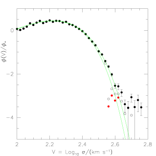
In all cases, the velocity dispersions were derived from the SDSS spectra (median signal-to-noise S/N=18 per pixel) and aperture corrected to $R_{e}/8$ as described by Bernardi et al. (2006). Figure 8 shows the distribution of objects as a function of velocity dispersion, in the SDSS, using methods detailed in Sheth et al. (2003). Symbols with error bars show the measured distribution before removing the objects which are superpositions - notice the apparent excess at $\sigma\geq 350$ km s^-1; open circles show the result of removing superpositions identified on the basis of SDSS imaging and spectra (following Bernardi et al. 2006), so they overestimate the true abundances; and filled circles without error bars show the result of assuming that the only single objects are those identified by our HST analysis - so they underestimate the true abundances. This shows that superpositions do affect the large $\sigma$ tail significantly, but that, once they have been removed, there is no excess of objects at high $\sigma$. The single galaxy with the largest aperture corrected velocity dispersion has a spectrum with S/N=25, is located in a group environment at $z=0.25$, and has $\sigma_{c}=426\pm 30$ km s^-1.

It is worth discussing the toe of large $\sigma\approx 500$ km s^-1 ($\log\sigma\approx 2.7$) objects in a little more detail. Such a toe is not seen in Figure 1 of Sheth et al. (2003) because the SDSS database at the time set a hard upper limit on reported dispersions of $\sigma=414$ km s^-1. This is still true: objects for which the pipeline would have returned a larger $\sigma$ are simply assigned this limiting value, $\sigma=414$ km s^-1, in the database. For this reason, Figure 8 in the current draft is based on our own reductions of the objects which SDSS reports as having $\sigma>350$ km s^-1 (Bernardi et al. 2006). These reductions are essentially the same as those of the SDSS, except that we use the actual values returned by our analysis pipeline even if they exceed $\sigma=414$ km s^-1.

The Sheth et al. (2003) analysis was based on a small enough sample that this limiting value affected only a handful of objects, so the toe associated with objects piling up at 414 km s^-1 was not obvious. The toe is there in the larger sample, as our Figure 8 shows. Of course, we also argue that this toe is almost entirely made up of doubles rather than singles. The two smooth curves show an estimate of the intrinsic distribution, and the result of convolving it with measurement errors.

Figure 9: Top: Distribution of Mg₂ index strength in our sample of 43 objects. Shaded, solid and dashed histograms are for objects classified as singles, doubles and multiples. Bottom: Strength of Mg₂ index as function of velocity dispersion. Circles represent the singles, squares show the doubles, and squares with an additional cross show objects which are superpositions of more than two components. Note the relatively clear separation between the doubles and the others. The hashed regions show the relation defined by the bulk of the early-type galaxy population at two different redshifts. The big-$\sigma$ singles populate the upper end of the relationship defined by the bulk of the population.

2.6 The Mg$-\sigma$ relation

Bernardi et al. (2006) suggested that early-type galaxy scaling relations (e.g. $R-L$, $R\sigma^{2}-L$) could be used as a diagnostic for superposition. The objects in this sample, however, all lie sufficiently close to these relations that Bernardi et al. were unable to separate the singles from superpostions.

Bernardi et al. (2006) also argued that correlations between absorption line indices and velocity dispersion should provide an efficient way of identifying superpositions. The idea is that superpositions which affect the measured $\sigma$ will also affect the measured line index strengths. For the Mg${}_{2}-\sigma$ relation, for example, objects in close superposition are expected to lie below and to the right of the true relation. This was the technique for which the precise place to divide between singles and superpositions was least robustly determined. Now that we have the HST imaging to identify the superpositions, we can ask how well this technique works.

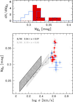
Figure 9 shows the Mg${}_{2}-\sigma$ relation for our sample. Note the clear separation between singles (filled circles) and doubles (open squares): at a given $\sigma$, doubles do indeed have abnormally low Mg₂. For comparison, shaded regions show the relations defined by SDSS galaxies in two redshift bins: $0.04<z<0.07$ (black) and $0.15<z<0.20$ (grey). The singles lie at the large $\sigma$ extremes of these relations, a point we will return to later. On the other hand, notice that the squares with crosses populate the same regions as the filled circles: evidently, this method alone is not effective at isolating objects with more than two components.

3 The shapes of singles: Evidence for two populations?

The same galaxy, if viewed along its longest axis, will appear rounder, with a larger velocity dispersion and smaller size, than if the line of sight is perpendicular to the longest axis. So it is interesting to ask if the large velocity dispersions in our sample are due in part to projection effects. If so, then this may indicate that they formed from primarily radial orbits (e.g. González-García & van Albada 2005; Boylan-Kolchin et al. 2006).

Figure 10: Top: Distribution of luminosities for galaxies classified as singles. Countours show the distribution of the early-type galaxy sample of Bernardi et al. (2006). Solid line contours include $68\%$ of the objects. Filled circles and open diamonds in the panel on the left show objects classified as ‘round’ and ‘elongated’; crosses and triangles in the panel on the right represent galaxies in high and low density environments. Bottom: Axis ratio $b/a$ versus luminosity. Symbols and contours as in upper panels. Small stars show the distribution of the BCG sample used in Bernardi et al. (2007a).

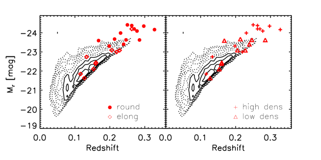
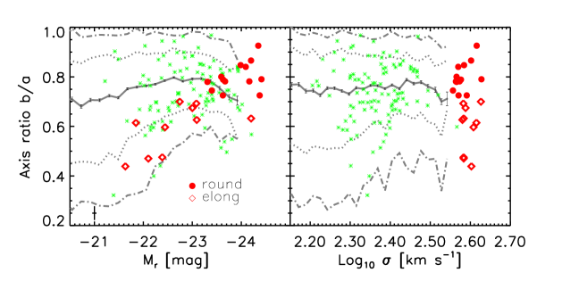
All the single galaxies in our sample were classified as being ‘round’ if the SDSS axis ratio parameter $b/a>0.7$, and as being ‘elongated’ otherwise. This classification is consistent with a visual inspection of the isophotal structure in the ACS $i$-band image. The top panels of Figure 10 show the distribution of luminosities as a function of redshift; circles and diamonds show ‘round and ‘elongated’ galaxies. Notice that there are no round objects at low redshift. What causes this?

Vincent & Ryden (2005) have analyzed the shapes of $z\leq 0.12$ ellipticals in SDSS DR3, and find that the most luminous galaxies are rounder. This is consistent with work prior to the SDSS (e.g. Tremblay & Merritt 1996). The top left panel in Figure 10 shows that the distribution of luminosities in our sample increases strongly with redshift (a consequence of the SDSS magnitude limit), and that the more luminous objects are indeed rounder.

Figure 11: The velocity dispersion-luminosity relation. Symbols with error bars show the median $\sigma$ in small bins in $L$ for the bulk of the early-type population, dotted and dot-dashed lines show the region populated by 68% and 95% of the galaxies. Thick solid line shows a linear fit to this distribution to emphasize the flattening at high-$\sigma$. Small stars show the BCGs, and the other symbols show our big-$\sigma$ sample. Filled circles and open diamonds in the panel on the left show objects classified as ‘round’ and ‘elongated’; triangles and crosses in the panel on the right indicate low and high density environments.

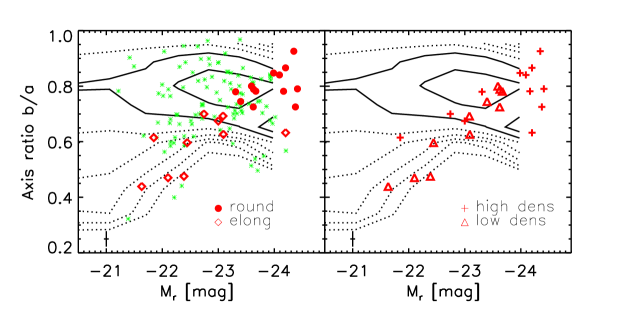
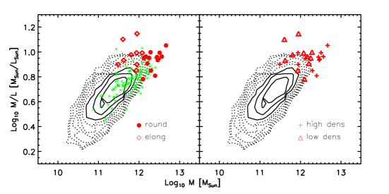
To quantify if there is a real trend, we must compare the shapes in our sample with the expected shapes of galaxies of the same luminosity but less extreme velocity dispersions. This is done in the bottom left panel of Figure 10. Contours show the distribution of the bulk of the early-type population in the $b/a$-luminosity plane; the transition from solid to dotted lines delineates the region containing $68\%$ of the objects. At luminosities fainter than $M_{r}=-22$ this distribution broadens, so the mean $b/a$ decreases – this is responsible for most of the luminosity dependence we referred to previously. Here, we are most interested in the brighter objects ($M_{r}\la-22$) where, to lowest order, the distribution of $b/a$ appears to be almost independent of luminosity. There is a hint of a decrease at the very bright end ($M_{r}\la-23.5$), a point to which we will return shortly.

For comparison, stars show the shapes of the BCGs in the SDSS C4 sample analyzed by Bernardi et al. (2007a); BCGs appear to have approximately the same distribution as the main galaxy sample – but note that they too appear to have slightly smaller $b/a$ at $M_{r}<-23.5$. If we ignore this decrease, then the plot indicates that all but one of the big-$\sigma$ objects more luminous than $M_{r}=-23.1$ is ‘round’, and all of the fainter objects are ‘elongated’. In fact, the ‘round’ objects in our sample tend to have values of $b/a$ which are about typical for their luminosity, whereas many of the others have lower than average $b/a$.

The bottom panel on the right shows that, at fixed $L$, the big$-\sigma$ objects in high-density environments have larger $b/a$ (i.e., are rounder) than their counterparts in low-density environments, an interesting finding that we will not pursue further here.

Figure 12: Shape parameter $b/a$ as a function of luminosity (left) and velocity dispersion (right) for the bulk of the early-type population; thick solid line shows the median, dotted lines show the region populated by 68% of the galaxies, and dot-dashed lines show the same but for 95%. Stars show the distribution of BCGs and circles and diamonds show our big-$\sigma$ sample.

Figure 13: Correlation between axis ratio $b/a$ and residuals from the mean $\sigma$ in two narrow bins in luminosity for the bulk of the early-type galaxy population. Filled circles show the median, dotted lines show the region populated by 68% of the galaxies, and dot-dashed lines show the same but for 95%. At low luminosities objects which have small $\sigma$ for their $L$ are slightly rounder; at high luminosities, the objects which have large $\sigma$ for their $L$ are rounder (they have large $b/a$). Note also that the scatter in $\sigma$ is smaller at large $L$.

3.1 Fast rotators at low luminosities?

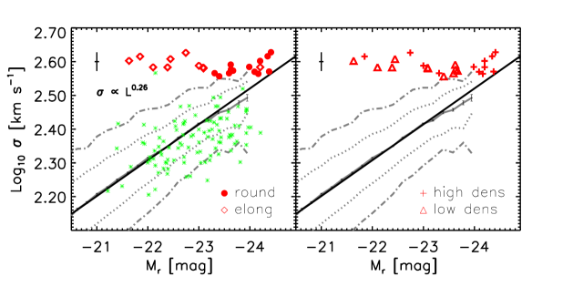
Figure 11 shows the velocity dispersion-luminosity relation traced by these objects. This illustrates that the high-luminosity objects outline the high-$\sigma$ boundary of the relation defined by the bulk of the population, whereas the low-luminosity objects are clearly extreme outliers. These are primarily the ‘elongated’ objects, for which projection effects cannot have caused the large velocity dispersions. E.g., if the objects are prolate, then small $b/a$ means the long axis is perpendicular to the line of sight, so the velocity dispersion is not enhanced. If the objects are oblate, then small $b/a$ suggests they may be like thick disks viewed edge-on. The SDSS velocity dispersion estimate comes from a single fiber, so it does not separate out the contribution to the observed velocity dispersion $\sigma$ which comes from ordered motions $v$. Hence, one might wonder if rotational motion $v$ has contributed to the velocity dispersion estimate of the low luminosity, big-$\sigma$ objects with small $b/a$.

Although spatially resolved spectra would allow us to address this definitively, a more detailed study of the HST surface brightness profiles of these objects, in Hyde et al. (2008), is very suggestive. Hyde et al. find that the most luminous objects tend to have shallower ‘core’ inner profiles, whereas the less luminous objects tend to have ‘power-law’ profiles with diskier isophotes. (We provide this core/power-law classification in Table 1; in most cases, the difference between ‘core’ and ‘power-law’ is already apparent in the contour plots shown in Figures 1–6.) This dependence on luminosity is in good agreement with previous HST-based work on early-type galaxies (e.g. Faber et al. 1997; Laine et al. 2003; Ferrarese et al. 2006; Lauer et al. 2007). In the present context, it is significant that power-law objects tend to have higher rates of rotation (Faber et al. 1997).

Moreover, there has been much recent interest in the distinction between slow rotators which tend to be luminous, and fast rotators which are not (e.g. Kormendy & Bender 1996; Cappellari et al. 2007). The flatter galaxies in our sample ($b/a\leq 0.6$) must have some degree of rotational support. E.g., Binney (1978, 2005) suggests that $(v/\sigma)\approx(1-b/a)/(b/a)$. Since the SDSS velocity dispersion estimate does not separate out the contribution from $v$ to the spectra, interpretation of the SDSS $\sigma$ for these objects is complicated. We can get a rough idea of the size of the effect by noting that, for an isotropic oblate rotator with $b/a=0.6$, rotation adds 21% to the total kinetic energy (Table 3 in Bender, Burstein & Faber 1992); if $b/a=0.5$, this factor is 33%. If there is a disk, then this factor can be even larger.

The SDSS spectra will be affected by this $v$ only if the light from the rotating component is a significant fraction of the total light in the fiber (also see Dressler & Sandage 1983 for a discussion of the effect of rotation on the estimated $\sigma$). Hyde et al. (2008) also provide bulge-disk decompositions of these objects. The elongated objects typically have bulge-to-total light ratios of order B/T$\approx 0.5$. The half-light radii of the bulges are approximately equal to B/T times the values reported in Table 2 (which are from single component fits). If there is a disk, then it is likely that the bulge is also rotating, and this will contribute to the SDSS estimate of $\sigma$. Moreover, for many of these objects, the angular half light radius of the bulge is slightly smaller than that of the SDSS fiber, so the dynamics of the disk may also have affected the spectrum. Thus, it seems likely that some of the flattening of the less luminous objects in our sample is due to rotation, and that the velocity dispersion estimate has been enhanced because of this rotation.

Figure 14: The color-magnitude relation of the bulk of the early-type population (solid, dotted and dot-dashed lines), the big-$\sigma$ sample (large symbols and dashed line) and BCGs (small stars). Line and symbol styles are as in Figure 11. The reddest object in the Figure has a dust-lane.

3.2 Radial mergers at high luminosities?

With this possibility in mind, it is worth reconsidering the $b/a-$luminosity and $b/a-\sigma$ relations. The panel on the left of Figure 12 shows the $b/a-$luminosity distribution, but now the solid curve shows the median $b/a$ for the bulk of the early-type population (defined for this figure as having $\sigma<350$ km s^-1) in a number of narrow bins in luminosity. The dotted and dot-dashed curves indicate the regions containing 68% and 95% of the objects in each luminosity bin. This shows that the gradual increase of $b/a$ with increasing $L$, that is consistent with previous work, reverses at $M_{r}\la-23.5$. The BCGs appear to track this reasonably well (suggesting that it would be interesting to repeat the analysis of BCG shapes in Ryden et al. 1993, in which luminosity dependence was ignored). If BCGs, or, more generally, the most luminous galaxies, formed from predominantly radial mergers, then one might expect them to be more prolate on average than the lower luminosity progenitors from which they formed. Thus, the decrease in the mean $b/a$ at large luminosities may be indicating that the radial merger model is reasonable.

The panel on the right shows a similar analysis of the $b/a-\sigma$ relation. In this case, the bulk of the population (defined as having $\sigma<350$ km s^-1) shows no trend, except for a slight decrease at $\log_{10}\sigma\ga 2.5$. Although the four BCGs with the largest values of $\sigma$ lie below this relation, a larger sample is needed to conclude that this decrease in $b/a$ at large $\sigma$ is also seen in the BCG population.

Notice that, in both panels, essentially all the ‘round’ big-$\sigma$ objects lie above the mean relation for their luminosities or velocity dispersions, whereas all the ‘elongated’ objects lie below it. If the velocity dispersions of the elongated objects have indeed been overestimated, then they should really be shifted to lower $\sigma$ (with no change in $L$). And if $b/a$ is an indicator of $v/\sigma$, this shift is of order 0.08 dex (see Section 3.1). However, the big-$\sigma$ objects which we classified as being ‘round’ would not be shifted. Because they are rounder than expected given the $b/a-L$ and $b/a-\sigma$ scalings for the bulk of the population, we cannot reject the hypothesis that these objects are prolate and viewed along the line of sight, and this has enhanced the observed velocity dispersions. However, we argue below that this enhancement is unlikely to be more than a 10% effect.

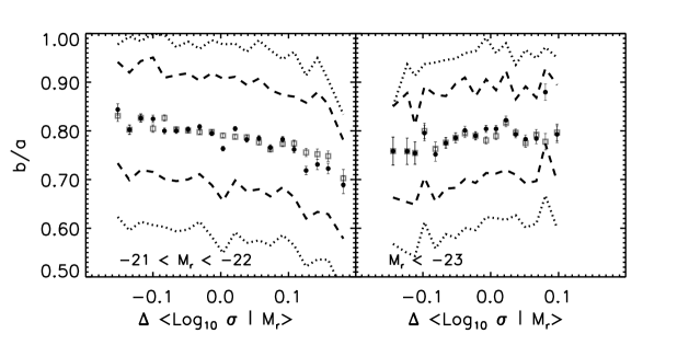
If the velocity dispersions have been enhanced by projection, we might expect projection effects to contribute to the scatter in the $\sigma-L$ relation. Figure 13 shows the correlation between axis ratio $b/a$ and residuals from the mean $\sigma$ in two narrow bins in luminosity for the bulk of the early-type galaxy population. At low luminosities objects which have small $\sigma$ for their $L$ are slightly rounder (they have larger $b/a$). This trend reverses at high luminosities, where the objects which have large $\sigma$ for their $L$ are rounder. The sense of the scaling at large $L$ is expected in the projection model.

Figure 15: Mg₂ index as function of velocity dispersion (left), r-band luminosity (middle) and effective radius (right). The flattened low luminosity objects (open symbols in top panels) have substantially larger Mg₂, so that Mg₂ is now anti-correlated with luminosity and size. Bottom panel shows that cluster galaxies tend to have larger Mg₂ than more isolated galaxies of the same $L$.

We show below that the mean $M_{\rm dyn}-L$ relation has small scatter, even at large $L$ (Figure 17). If the long axis of a prolate object is perpendicular to the line of sight, then $R\propto\sqrt{ab}$, whereas $R\propto b$ if it lies along the line of sight. If $\sigma$ were the same in both cases, then the two dynamical mass estimates would differ by a factor of $\sqrt{b/a}=0.84$ ($0.08$ dex) if $b/a=0.7$ (which Figure 12 indicates is the mean value at $M_{r}<-23.5$). This shows that projection effects could contribute substantially to the scatter in the $M_{\rm dyn}-L$ relation. However, if the observed $\sigma$ is larger when viewed along the long axis (as one expects from the virial theorem), then the variation in the $M_{\rm dyn}$ estimate that is due to projection effects decreases (e.g. González-García & van Albada 2005). Since it is $\sigma^{2}$ which matters here, a $0.08$ dex variation in the size due to orientation effects could be cancelled by a $0.04$ dex variation in Log₁₀($\sigma$). The scatter in $\sigma$ decreases at large $L$ (see Figure 11, or compare the range in the two panels of Figure 13, or see Figure 3 in Sheth et al. 2003); at $M_{r}<-23$ the observed rms scatter is 0.05 dex, of which about 0.03 dex is not due to measurement errors. It is interesting that this is about the level expected if projection effects are beginning to dominate the scatter in the $\sigma-L$ relation.

3.3 Colors, projection and dust

A possible problem with the projection model is that the most luminous objects in SAURON tend to be oblate, not prolate (Cappellari et al. 2007). If our objects are oblate, then the round shapes we see ($b/a\geq 0.8$) suggest that we are seeing them face on, making the line of sight axis the shortest, rather than the longest one. Therefore, as another test of the projection model for the ‘round’ objects in our big-$\sigma$ sample, we have studied their colors.

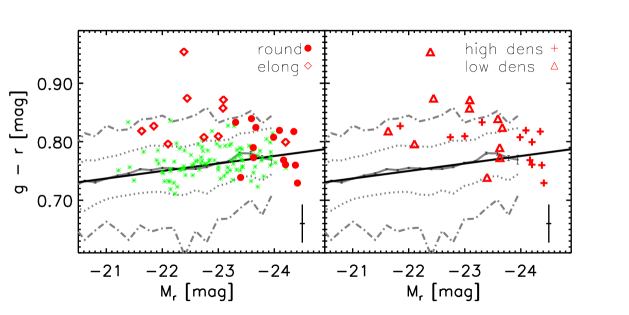
For the bulk of the early-type galaxy population, the color-magnitude relation is flat at fixed $\sigma$, with mean color increasing with $\sigma$ (Bernardi et al. 2005). The filled circles in the left-hand panel of Figure 14 show that, indeed, the round galaxies in our sample define a flat color-magnitude relation. If there were no dust, then one would not expect the colors to be affected by projection effects. On the other hand, if these objects are dusty, prolate BCGs, viewed along the line of sight, one might expect them to appear redder than BCGs of the same $L$. Figure 14 suggests that they are not redder than BCGs, so if they are dusty, it will be difficult to accomodate the projection model. One would then have to argue that they are intrinsically slightly bluer – perhaps as a consequence of dry mergers of objects which were on similar positions in the color-magnitude relation. The merger would increase the luminosity without changing the color, so moving them slightly brightward with respect to the color-magnitude relation. At fixed luminosity, these objects would lie blueward of the mean relation if there were no dust; dust would bring them back onto the relation.

In contrast to the ‘round’ objects in our sample, about half of the ‘elongated’ objects have extremely red colors. However, the three reddest of these, SDSS J103344.2$+$043143.5, SDSS J112842.0+043221.7 and SDSS J082646.7+495211.5, have obvious dust lanes. (One other object, SDSS J082216.5+481519.1, also has a dust lane; see Hyde et al. 2008 for further study of these objects.) If these objects are fast rotators, then the presence of such dust lanes is not unexpected.

Figure 16: Correlation of size with luminosity for the bulk of the early-type population (solid, dotted and dot-dashed lines) and in our big-$\sigma$ sample (symbols and dashed line). Line and symbol styles are as in Figure 11. Stars show these correlations for BCGs.

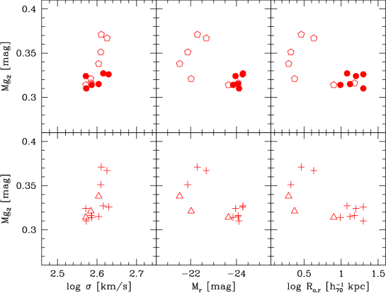
Furthermore, the fast rotators seen by SAURON have anomolously large Mg₂ index strengths which is thought to be caused by stars which formed from metal-enriched gas. Figure 15 shows that the flattened, low luminosity objects in our big$-\sigma$ sample (diamonds) also have abnormally large Mg₂ values; indeed Mg₂ is anti-correlated with luminosity and size. This suggests that, if rotation is important for these objects, then dissipation associated with the gastrophysics of star formation was also important. Recall that these flattened objects tend to be the reddest objects for their luminosity - they are substantially redder than BCGs (Figure 14). If Mg₂ is due to star formation, then it either happened long ago (else the colors would be bluer), or the redder colors are due to extreme metallicities or dust – which we know is playing some role in at least half of these objects.

3.4 Brief summary

To summarize this section, it appears that our sample of singles is made up of two populations. The more luminous objects tend to be rounder and sit in crowded fields; it is possible that they are prolate objects, in most cases BCGs, viewed along the line of sight, in which case their velocity dispersions may be slightly enhanced compared to if they were oriented perpendicular to the line of sight. The less luminous objects tend to be more flattened; if some of this flattening is due to rotation, then it may be that the velocity dispersion estimate has been enhanced because of this rotation.

4 Scaling relations at large $\sigma$

We now study if the scaling relations of singles with large $\sigma$ are significantly different from those defined by the bulk of the early-type population.

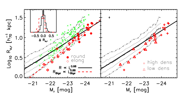
Figure 16 shows that, at the high luminosity end, these objects (diamonds and circles) tend to be similar to the bulk of early-types (solid, dotted and dot-dashed lines), if one ignores the curvature in the size-luminosity relation (thick solid line). However, the solid line with error bars show that the $R-L$ relation curves upwards at high luminosities. All our big-$\sigma$ objects lie below this curved relation. In addition, they are systematically smaller than BCGs (stars) of the same luminosity, whatever the luminosity.

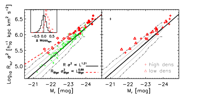
The top panels of Figure 17 show that these objects define a tight mass-luminosity relation (we set $M_{\rm dyn}\propto R\sigma^{2}$) that is offset from and has a different slope compared to that defined by the bulk of the population; they are the most massive galaxies at any $L$, even compared to BCGs. Only at the largest $L$ do BCGs have similar masses. This shows again (c.f. Figure 12) that the most massive galaxies in the Universe have large $\sigma$ and $L$. We discuss the different slope and offset shortly.

Figure 17: Correlation of dynamical mass (top) and density (bottom) with luminosity for the bulk of the early-type population (solid, dotted and dot-dashed lines) and in the big-$\sigma$ sample (symbols and dashed line). Line and symbol styles are as in Figure 11. Stars show these correlations for BCGs.

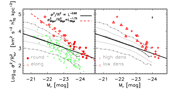
Since density $\propto(R\sigma^{2}/R^{3})\propto(\sigma/R)^{2}$, the large velocity dispersions and small sizes of these objects mean they are much denser than average galaxies of the same $L$. The bottom panels in Figure 17 show that the density-$L$ relation they define is indeed very different from that of the bulk of the population. Note in particular that they are typically about 0.6 dex denser than BCGs of the same luminosity. At low luminosities, they appear to be more than ten times denser than average. We will have more to say about this shortly.

The mass-luminosity and density-luminosity scalings are approximately consistent with the $R\propto L^{0.9}$ scaling, and the assumption that $\sigma$ is essentially constant, since this would predict mass $\propto R\sigma^{2}\propto L^{0.9}$, and density $\propto(\sigma/R)^{2}\propto L^{-1.8}$. Hence, to understand these other scalings, it is sufficient to understand why $R\propto L^{0.9}$, when the bulk of the population scales as $R\propto L^{0.68}$. In this context, it is instructive to study the mean size at fixed $L$ and $\sigma$ in the bulk of the population.

We have done this in two ways, one numerical, and the other analytic. First, following arguments in Bernardi et al. (2005),

$$\frac{\langle R|M_{r},V\rangle}{\sigma_{R}}=\frac{M_{r}}{\sigma_{M}}\frac{\rho_{RM}-\rho_{RV}\rho_{VM}}{1-\rho^{2}_{VM}}+\frac{V}{\sigma_{V}}\frac{\rho_{RV}-\rho_{RM}\rho_{VM}}{1-\rho^{2}_{VM}},$$ (1)

where $R$ and $V$ mean ${\rm log}(R/R_{*})$ and ${\rm log}(\sigma/\sigma_{*})$, $M_{r}$ is absolute $r-$band magnitude minus $M_{*}$, $\sigma_{x}$ is the rms of the observable $x$, and $\rho_{xy}$ is the correlation coefficient of the observables $x$ and $y$. Hence, at fixed $\sigma$, the slope of the size-magnitude relation is

$$\frac{\delta\langle R|M_{r},V\rangle}{\delta M_{r}}=\frac{\sigma_{R}}{\sigma_{M}}\,\frac{\rho_{RM}-\rho_{RV}\rho_{VM}}{1-\rho^{2}_{VM}}=\frac{-0.88}{-2.5},$$ (2)

where we have inserted the values derived from the $R-L$, $\sigma-L$ and $R-\sigma$ relations defined by the early-type sample.

Figure 18: Location of the big$-\sigma$ sample (circles and diamonds) with respect to the Fundamental Plane defined by the early-type galaxy sample (contours); stars show the location of BCGs. Contours and symbols as in Figure 10.

Second, we restricted the full sample to narrow bins in $\sigma$ and measured the slope of the $R-L$ relation in the different subsamples. We found that the slope does not depend on the choice of bin. The result of shifting the zero-point to best-fit our big$-\sigma$ sample is shown as the dashed line in the panel on the left of Figure 16. A similar analysis of the mass-$L$ and density-$L$ relations yields the dashed lines shown in Figures 17. In all cases, the dashed lines provide a good description of our big-$\sigma$ sample.

Figure 19: Distribution in $\kappa$-space (top panels: $\kappa_{2}$ versus $\kappa_{1}$; bottom panels: $\kappa_{3}$ versus $\kappa_{1}$) of the bulk of the early-types (contours), the big-$\sigma$ subsample, and BCGs. Contours and symbols as in Figure 10. The figure shows $\kappa_{1}$, $\kappa_{2}$ and $\kappa_{3}$ transformed to solar units. Dashed line sloping down and to right in top panels shows $\kappa_{1}+\kappa_{2}=8$ transformed to these variables.

Thus, both numerical and analytic arguments reproduce the steeper $R\propto L^{0.9}$ scaling of our big-$\sigma$ sample. So it seems reasonable to conclude that the objects in our big$-\sigma$ sample are simply the large$-\sigma$ extremes of the early-type population – they are not unusual in any other way (except, perhaps, their shapes). The underlying physical reason for this steeper relation can be understood as follows: If $R\sigma^{2}$ is linearly proportional to galaxy mass, then $(M/L)\,L=R\sigma^{2}$. So, at fixed $\sigma$, we expect $R\propto(M/L)\,L$. If the mass-to light-ratio were the same for all galaxies, then we would expect $R\propto L$, which is considerably steeper than the $R\propto L^{0.68}$ scaling which holds when one averages over all values of $\sigma$ in the population.

It is interesting to contrast these scalings with the size-luminosity relation of BCGs. The abnormally large sizes of BCGs suggest unusual formation histories - perhaps dominated by dry-mergers (e.g., Lauer et al. 2007; Bernardi et al. 2007a). So one might have wondered if the smaller sizes of the objects in our sample point to formation histories which are unusual in some other way. The discussion above suggests that their distribution in the size-luminosity plane is no more unusual than one might have expected, given their unusually large velocity dispersions. Since we already know they have large velocity dispersions – that is how this sample was selected – the size-luminosity relation contains no new information.

Thinking of these objects as having fixed $\sigma$ also helps understand the location of these objects with respect to the Fundamental Plane defined by the bulk of the population (see Figure 18): in essence, these objects trace out the size – surface-brightness correlation, with zero-point set by the value of $\sigma$. In this respect, the Fundamental Plane is not as useful a diagnostic of the properties of these galaxies as were the other scaling relations.

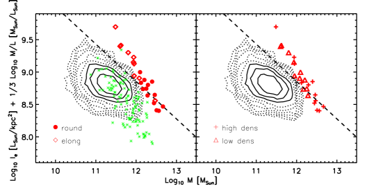
Although the FP itself was not particularly informative, the $\kappa-$space projection (Bender, Burstein & Faber 1992) is. The bottom panels in Figure 19 (the edge-on projection) show that the round objects in our sample have mass-to-light ratios which are similar to those of BCGs; they are slightly larger than those of the bulk of the population. However, some of the elongated objects appear to have mass-to-light ratios that are even larger than those of BCGs. The face-on projection (top panels) shows that while the round objects in our sample lie close to the boundary of the zone-of-avoidance ($\kappa_{1}+\kappa_{2}\geq 8$) defined by the bulk of the population, the elongated objects lie well inside it. Bender et al. associated this boundary with extreme dissipation, so Figure 19 suggests that the lowest mass, elongated objects in our big$-\sigma$ sample have undergone abnormally high amounts of dissipation.

However, most of these abnormal objects have small $b/a$, so one might worry that this conclusion changes if they are indeed fast rotators. In this case, the SDSS $\sigma$ is almost certainly an overestimate, making both the estimated mass and density larger than they really are. Accounting for this will reduce the $M/L$ values and shift the position in the face-on view of $\kappa$-space, thus weakening the case for extreme dissipation. To estimate the magnitude of this effect, we can use the bulge-disk decompositions in Hyde et al. (2008). These suggest bulge sizes are typically about a factor of 2 smaller than reported here, whereas bulge luminosities are reduced by a smaller factor. If we also correct the velocity dispersions downwards by about 20% (see discussion in Section 3.1), then the net effect is to increase the density by 0.4 dex while making the magnitudes somewhat less than 0.75 mags fainter. Thus, the bulges will be closer to the $\kappa_{1}+\kappa_{2}=8$ boundary, but will remain the densest objects for their luminosities.

5 Discussion

We used HST imaging (Figures 1–6) to separate genuinely single objects from those which are superpositions in a sample drawn from the SDSS DR1 and chosen to have $\sigma\geq 350$ km s^-1. The abundance of these large $\sigma$ objects that are singles is consistent with that given by extrapolating fits to the SDSS velocity function to higher $\sigma$ – there is no ‘toe’ at $\sigma>400$ km s^-1 (Figure 8).

The scaling relations (size-$L$, mass-$L$ and density-$L$) defined by these objects are different from those defined by the bulk of the early-type galaxy population: for a given luminosity, these objects are amongst the most massive and densest early-type galaxies (Figures 16 and 17). However, these differences can be understood by thinking of this sample as being the large-$\sigma$ tail of the early-type galaxy population, but not being otherwise unusual. Table 2 lists the redshifts, luminosities, sizes, velocity dispersions, colors, Mg₂ abundances, shapes, and environments of these objects. (The luminosities, sizes and shapes have been corrected for known problems with SDSS sky-subtraction; Section 2.3).

These single galaxies with $\sigma\geq 350$ km s^-1 appear to be of two types: the more luminous objects ($M_{r}<-23.5$ or so) are round ($b/a>0.7$), whereas the less luminous objects are flatter (Figure 10). In addition, Hyde et al. (2008) show that the HST-based surface brightness profiles of the low and high luminousity objects are ‘power-laws’ and ‘cores’ (in the language of Faber et al. 1997); the trend with luminosity is consistent with previous HST work on the centres of early-type galaxies, which shows that power-law galaxies may have significant rotation. The cores, in the galaxies which have them, are about a factor of ten smaller than the half-light radii. However, the cores are not unusually small for the total $L$ or $\sigma$ (Hyde et al. 2008); this is in contrast to the half-light radii, which are (Figure 16). On the other hand, if the objects we classify as power-laws actually have cores that are below our resolution limit, then the upper limits we can set to the core-size are already at the low-end of the expected sizes for their $\sigma$, and perhaps also for their $L$ (Hyde et al. 2008).

What do our observations imply for the formation histories of these two populations? At large $L$, these objects tend to be found in crowded fields so they may be BCGs. If so, then it is likely that they formed from merging or accreting smaller galaxies, and this would explain why their inner profiles are shallow. The puzzle is to explain why these objects are so much denser than the average galaxy or BCG of the same $L$ (bottom panels of Figures 17 and 18), especially since the sizes of the inner core radii appear to be normal – they do not appear to be small for their $L$ or $\sigma$ (Hyde et al. 2008). One possibility is that these objects formed from predominantly radial mergers with little angular momentum. If the prolate objects which result are viewed along the long axis, this would produce slightly smaller half-light radii and slightly larger velocity dispersions.

In this context, it is worth noting that the trend for the mean shape to become increasingly round as luminosity increases (e.g., Vincent & Ryden 2005) appears to reverse at $M_{r}<-23.5$ (Figures 12 and 13). This appears to be true for galaxies in the main sample, and for BCGs – and is in qualitative agreement with models which postulate that radial mergers are common at large luminosities. Compared to this decrease in $b/a$ at large $L$, the luminous objects in our big-$\sigma$ sample appear to be rounder than expected (Figure 12), consistent with the hypothesis that projection effects have resulted in smaller sizes and larger velocity dispersions. Nevertheless, even if one accounts for this effect, these objects are amongst the densest BCGs for their luminosities.

Whereas projection effects may be important at large $L$, they almost certainly cannot account for the flattened shapes we see at low $L$. We can think of two plausible models for these flattened objects.
i) These are objects which contain a substantial component that is rotationally supported.
ii) These are objects in which gaseous dissipation has been most efficient.
Option (i) must matter for the objects with $b/a\leq 0.6$, since anisotropic dispersions cannot produce extremely flat shapes. Indeed, the fact that we see small $b/a$ only at small $L$ (Figure 10) suggests that these are examples of the low luminosity, fast-rotator population which has received considerable recent attention from e.g., the SAURON group (Cappellari et al. 2007). If so, then the SDSS velocity dispersions are artificially broadened by rotational motions, thus affecting the mass and density estimates. Reducing the mass estimates by the appropriate $b/a$-dependent factor would bring the flattened objects closer to the relation defined by the bulk of the population; it would also bring the objects closer to the $\kappa_{1}+\kappa_{2}=8$ boundary in $\kappa-$space (Figure 18).

Further indirect evidence for rotation comes from Hyde et al. (2008) who show that these objects have ‘power-law’ inner profiles, and significant amounts of dust. Previous work has shown that such objects often have a significant rotational component (e.g. Laine et al. 2003). Determining if this is the case for our sample requires spatially resolved kinematics. Nevertheless, we argue that even if one accounts for rotational motions, these objects are likely to remain the densest for their luminosities. Thus, it appears that both (i) and (ii) are true for these objects (e.g., Figure 15 and related discussion).

If the lower luminosity objects are indeed contaminated by rotation whereas the higher luminosity objects are not, then one might ask if the fact that both low and high luminosity objects define the same power-law scaling relations (Figures 16–19) is simply fortuitous. However, both rotational and random motions contribute to the kinetic energy in the virial theorem. E.g., Appendix B of Bender, Burstein & Faber (1992) suggests that using only the true $\sigma$ of an isotropic oblate rotator underestimates the true mass by 35% if $b/a=0.6$. In addition, recent work on the velocity dispersion estimates of more distant objects suggests that including the effect of rotation on mass estimates may indeed be important (e.g. van der Vel & van der Marel 2008). So it may be that the contribution of ordered motions to SDSS velocity dispersion estimates helps to keep the scaling relations power-laws. In this regard, when comparing our sample of high-velocity dispersion galaxies with higher redshift z$\sim$1.5 samples of passive galaxies (Figure 19 in Cimatti et al. 2008), the lower-luminosity galaxies in our sample populate a similar locus in the size, mass, surface density plane as the superdense z$\sim$1.5 passive galaxies. It is possible that our low-redshift high-density galaxies are the rare examples of the high-redshift superdense galaxies which have not undergone any dry merging. This scenario is supported by the fact that the low luminosity galaxies in our sample are in low-density environments and have intact power-law centers. So it would be interesting to check if the superdense z$\sim$1.5 galaxies are “fast-rotators”.

It is common to predict black hole abundances by transforming an observed luminosity or velocity dispersion function using an assumed scaling relation between black hole mass $M_{\bullet}$ and galaxy $L$ or $\sigma$ (e.g. Lauer et al. 2007; Tundo et al. 2007; Shankar et al. 2008). If one ignores the fact that there is scatter around the mean $M_{\bullet}-L$ or $M_{\bullet}-\sigma$ relations, then one might conclude that the big-$\sigma$ sample studied here would predict higher black hole masses from their $\sigma$ than from their $L$s. However, the scatter is significant: the analysis in Bernardi et al. (2007b) shows how to include the possibility that the scatter in the $\sigma-L$ relation is correlated with scatter in the $M_{\bullet}-L$ and $M_{\bullet}-\sigma$ relations. See their Section 2.3 for a discussion of the effect of selecting objects with large $\sigma$ for their $L$.

Finally, we note that although we have focussed on the single objects in this sample, the superpositions are interesting in their own right. Because they are close superpositions in both angle and redshift, in which the spectra show little or no sign of recent star formation, and because they provide information about smaller scales than is possible with ground based data, they can be combined with other HST-based samples of early-type galaxies (e.g. Laine et al. 2003; Lauer et al. 2007) to constrain dry-merger rates more precisely than previously possible (e.g. Bell et al. 2006; Masjedi et al. 2007; Wake et al. 2008). Such combined samples can also be used to build more realistic models of the expected configurations of multiple-lens systems. These studies are in progress.

Table 2: Properties of the 23 objects identified as singles. Superscript $c$ means the inner profile is shallow core (from Hyde et al. 2008). Magnitudes, sizes, color and $b/a$ were computed by Hyde et al. (2008) on SDSS r-band images, while velocity dispersions and Mg₂ index-strenghts are from Bernardi et al. (2006).

IDS	$z$	$M_{r}$	$e_{M}$	$g-r$	$e_{g-r}$	log${}_{10}R$	$e_{R}$	$\sigma$	$e_{\sigma}$	Mg2	$e_{{\rm Mg}_{2}}$	$b/a$	$e_{b/a}$	Env
		[mag]	[mag]	[mag]	[mag]	[kpc]	[kpc]	kms-1	kms-1	[mag]	[mag]
1	0.23949	-23.40	0.06	0.74	0.04	1.00	0.03	360	37	–	–	0.74	0.04	0
$2^{c}$	0.19827	-23.31	0.04	0.84	0.03	0.93	0.02	367	28	–	–	0.78	0.03	1
$3^{c}$	0.16773	-23.59	0.03	0.84	0.02	1.09	0.02	367	29	0.307	0.010	0.80	0.02	0
$4^{c}$	0.32787	-24.16	0.06	0.78	0.05	1.32	0.03	366	52	–	–	0.78	0.04	1
$5^{c}$	0.27775	-24.09	0.05	0.83	0.04	1.24	0.03	371	30	0.324	0.009	0.84	0.04	1
$6^{c}$	0.21356	-23.67	0.04	0.83	0.03	0.89	0.02	374	22	0.314	0.008	0.78	0.02	0
$7^{c}$	0.26271	-24.38	0.04	0.77	0.04	1.36	0.02	372	29	0.310	0.009	0.73	0.03	1
$8^{c}$	0.24639	-23.63	0.05	0.78	0.04	1.04	0.03	377	33	–	–	0.79	0.03	0
9	0.20533	-23.09	0.06	0.88	0.04	0.86	0.03	380	34	–	–	0.63	0.03	0
10	0.22792	-23.08	0.05	0.86	0.04	0.71	0.03	382	27	–	–	0.69	0.04	0
11	0.15939	-22.39	0.04	0.96	0.03	0.72	0.02	383	41	–	–	0.48	0.02	0
12	0.15335	-22.10	0.05	0.80	0.03	0.39	0.03	383	28	0.321	0.008	0.47	0.03	0
$13^{c}$	0.26275	-24.20	0.04	0.81	0.03	1.24	0.02	383	34	0.316	0.009	0.63	0.02	1
$14^{c}$	0.23073	-23.99	0.03	0.81	0.03	1.06	0.02	384	32	0.314	0.009	0.85	0.03	1
15	0.21930	-23.00	0.06	0.81	0.04	0.71	0.03	387	41	–	–	0.67	0.04	1
16	0.28489	-23.62	0.07	0.80	0.05	0.96	0.04	390	44	–	–	0.73	0.04	0
17	0.12705	-21.63	0.05	0.82	0.03	0.34	0.02	400	28	0.338	0.010	0.44	0.02	0
$18^{c}$	0.26965	-24.20	0.05	0.77	0.03	1.20	0.03	399	35	0.315	0.009	0.87	0.03	1
19	0.11610	-21.85	0.03	0.83	0.02	0.20	0.02	412	27	0.351	0.009	0.61	0.02	1
20	0.16037	-22.44	0.04	0.88	0.03	0.53	0.02	405	26	0.371	0.009	0.60	0.03	0
$21^{c}$	0.29718	-24.35	0.04	0.82	0.04	1.10	0.02	412	27	0.327	0.007	0.93	0.03	1
$22^{c}$	0.13343	-22.74	0.02	0.81	0.01	0.63	0.01	423	31	0.367	0.010	0.70	0.02	1
$23^{c}$	0.25026	-24.41	0.04	0.74	0.03	1.35	0.02	424	30	0.326	0.006	0.79	0.02	1

References

- [] Abazajian, K., et al. 2003, AJ, 126, 2081
- [] Abbas, U. & Sheth, R. K. 2007, MNRAS, 378, 641
- [] Almeida, C., Baugh, C. M. & Lacey, C. G., 2007, MNRAS, 376, 1711
- [] Bell E., et al., 2006, ApJ, 652, 270
- [] Bender, R., Burstein, D. & Faber, S. M. 1992, ApJ, 399, 462
- [] Bernardi, M., Sheth, R. K., Nichol, R. C. et al. 2005, AJ, 129, 61
- [Bernardi et al.(2006)] Bernardi, M., Sheth, R. K., Nichol, R. C., Miller, C. J., Schlegel, D., Frieman, J., Schneider, D. P., Subbarao, M., York, D. G., Brinkmann, J. 2006, AJ, 131, 2018
- [Bernardi et al.(2007)] Bernardi, M., Hyde J. B., Sheth, R. K., Miller, C. J., Nichol, R. C. 2007a, AJ, 133, 1741
- [Bernardi et al.(2007b)] Bernardi, M., Sheth, R. K., Tundo, E, & Hyde, J. B. 2007b, ApJ, 660, 267
- [] Bernardi, M. 2007, AJ, 133, 1954
- [] Binney, J. 1978, MNRAS, 183, 501
- [] Binney, J. 2005, MNRAS, 363, 937
- [] Boylan-Kolchin M., Ma C.-P., Quataert E., 2006, MNRAS, 369, 1081
- [] Cappellari, M., Emsellem, E., Bacon, R. et al. 2007, MNRAS, 379, 418
- [] Cimatti, A., et al. 2008, A&A, 482, 21
- [] Crawford C. S., Allen S. W., Ebeling H., Edge A. C., Fabian A. C., 1999, MNRAS, 306, 857
- [] De Lucia, G., Springel, V., White, S. D. M., Croton, D. & Kauffmann, G. 2006, MNRAS, 366, 499
- [] Dressler, A. & Sandage, A. 1983, 265, 664
- [] Faber, S. M., et al. 1997, aJ, 114, 1771
- [] Ferrarese L. & Merritt D., 2000, ApJ, 539, L9
- [] Ferrarese, L., Cote, P., Blakeslee, J. P., Mei, S., Merritt, D., & West, M. J. 2006, submitted, arXiv:astro-ph/0612139
- [Fruchter & Hook (2002)] Fruchter, A. S., & Hook, R. N. 2002, PASP, 114, 144
- [] Gebhardt K. et al. 2000, ApJL, 539, 16
- [] González-García, A. C. & van Albada, T. S. 2005, MNRAS, 361, 1043
- [] Hoessel, J. G., Oegerle, W. R. & Schneider, D. P. 1987, AJ, 94, 1111
- [] Hyde, J., Bernardi, M., Fritz, A., Gebhardt, K., Nichol, R. C. & Sheth, R. K., 2008, MNRAS, submitted
- [] Hyde, J. & Bernardi, M. 2008, MNRAS, submitted
- [] Kormendy, J. & Bender, R. 1996, ApJ, 459, 57
- [] Laine, S., van der Marel, R. P., Lauer, T. R., Postman, M., O’Dea, C. P., & Owen, F. N. 2003, AJ, 125, 478
- [] Lauer, T. R., et al. 2007, ApJ, 662, 808
- [] Malumuth E. M. & Kirshner, R. P. 1981, ApJ, 251, 508
- [] —. 1985, ApJ, 291, 8
- [] Masjedi M., Hogg D. W., Blanton M. R., 2007, ApJ, submitted, (arXiv:0708.3240)
- [] Mo, H. J. & White, S. D. M. 1996, MNRAS, 282, 347
- [] Oegerle W. R. & Hoessel J. G. 1991, ApJ, 375, 15
- [] Postman M. & Lauer T. R., 1995, ApJ, 440, 28
- [] Ryden, B. S., Lauer, T. R. & Postman, M. 1993, ApJ, 410, 515
- [] Sandage A., 1976, ApJ, 205, 6
- [] Scott E., 1957, AJ, 62, 248
- [] Schombert J. M. 1987, ApJS, 64, 643
- [] —. 1988, ApJS, 328, 475
- [] Schweizer F. 1982, ApJ, 252, 455
- [] Shankar, F., Weinberg, D. H., & Miralda-Escudé, J. 2008, ApJ, submitted, arXiv/0710.4488
- [] Sheth R. K., Tormen G. 2002, MNRAS, 329, 61
- [] Sheth, R. K., Bernardi, M., Schechter, P. L., et al. 2003, ApJ, 594, 225
- [] Thuan T. X. & Romanishin W. 1981, ApJ, 248, 439
- [Tremblay & Merritt(1996)] Tremblay, B., & Merritt, D. 1996, AJ, 111, 2243
- [] Tundo E., Bernardi M., Hyde J. B., Sheth R. K., Pizzella A. 2007, ApJ, 663, 53
- [] van der Vel, A. & van der Marel, R. 2008, ApJ, in press, arXiv/0804.4228
- [] Vincent R. A., Ryden B. S. 2005, ApJ, 623, 137
- [] Wake D. et al. 2008, MNRAS, 387, 1045